
Constraining Parameter Uncertainty in Simulations of Water and Heat Dynamics in Seasonally Frozen Soil Using Limited Observed Data

Abstract
:1. Introduction
2. Materials and Methods
2.1. Study Site Description
2.2. Experimental Design
2.3. Model Description
2.3.1. Soil Water Processes
2.3.2. Soil Heat Processes
2.3.3. Soil Evaporation and Radiation Processes
2.4. GLUE Method Uncertainty Analysis
3. Results
3.1. Model Calibration Performance
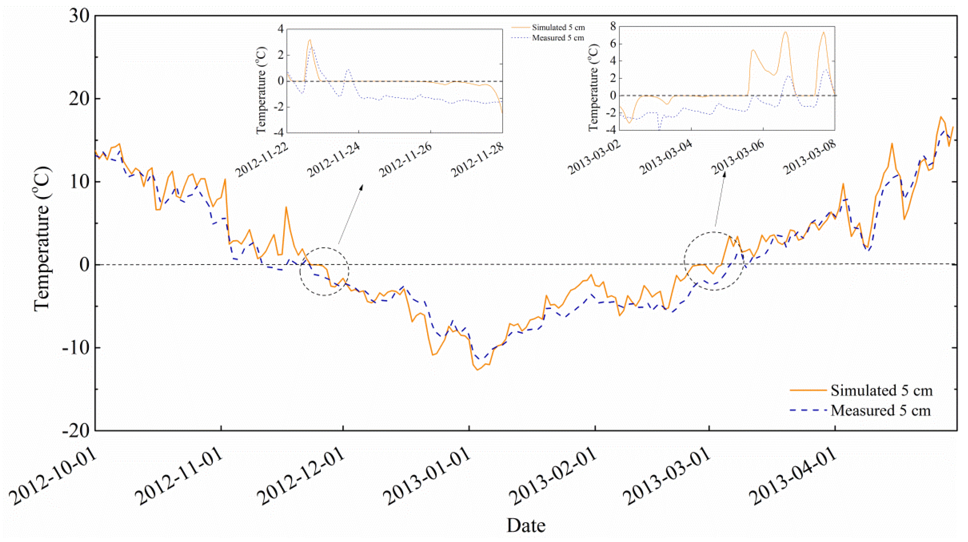
3.2. Simulation Results Based on Mean Values of Behavioral Parameters
3.3. Water Balance during Soil Freezing/Thawing
4. Discussion
4.1. Equifinality in Calibration of Frozen Soil Model
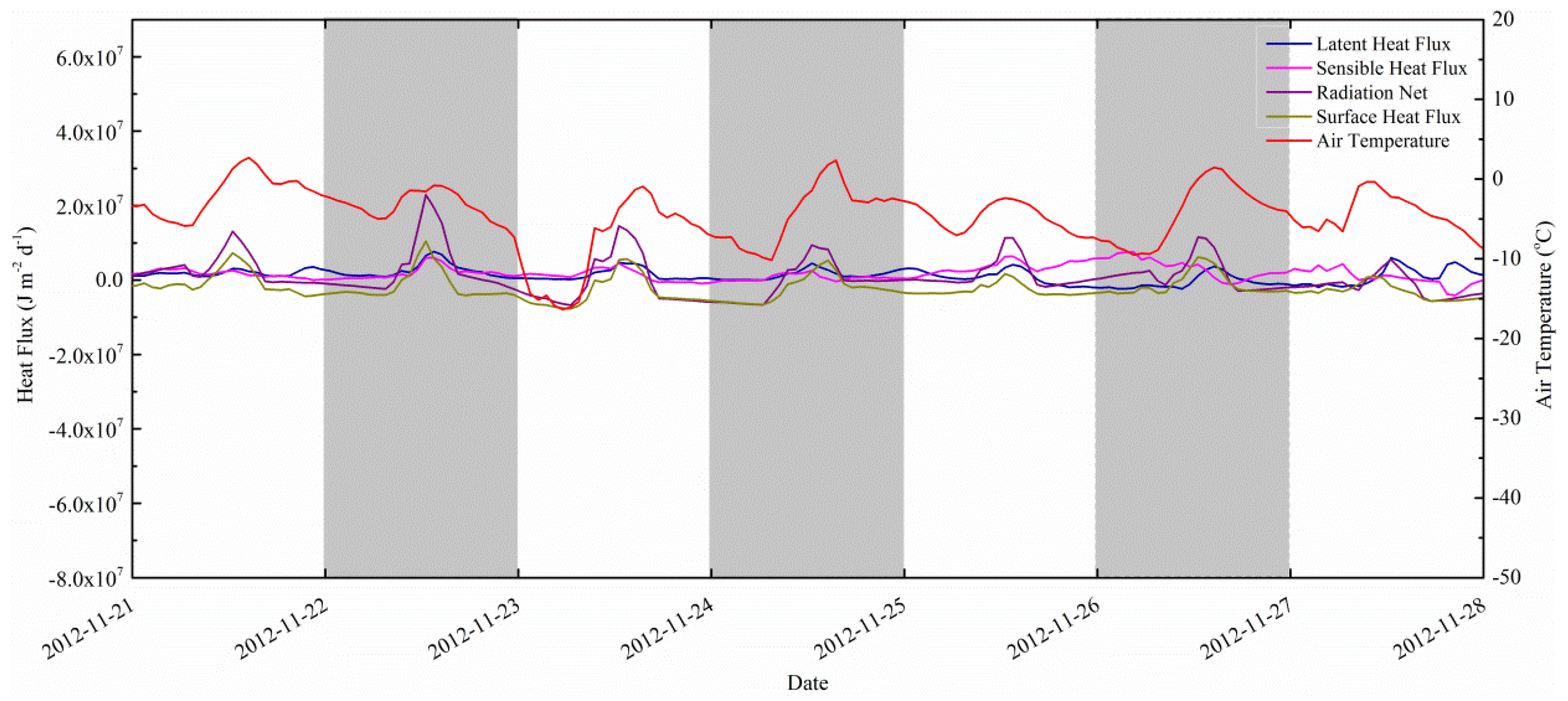
4.2. Seasonal and Diurnal Courses in Surface Energy Balance
5. Conclusions
Acknowledgments
Author Contributions
Conflicts of Interest
References
- Intergovernmental Panel on Climate Change (IPCC). Climate Change 2007—The Physical Science basis: Working Group I Contribution to the Fourth Assessment Report of the IPCC; Cambridge University Press: Cambridge, UK, 2007; Volume 4. [Google Scholar]
- Al-Faraj, F.A.M.; Scholz, M.; Tigkas, D. Sensitivity of surface runoff to drought and climate change: Application for shared river basins. Water 2014, 6, 3033–3048. [Google Scholar] [CrossRef]
- Wang, X. Vapor Flow Resistance of Dry Soil Layer to Soil Water Evaporation in Arid Environment: An Overview. Water 2015, 7, 4552–4574. [Google Scholar] [CrossRef]
- Lunardini, V.J. Heat Transfer in Cold Climates; Van Nostrand Reinhold Co.: New York, NY, USA, 1981. [Google Scholar]
- Wu, M.; Huang, J.; Wu, J.; Tan, X.; Jansson, P.-E. Experimental study on evaporation from seasonally frozen soils under various water, solute and groundwater conditions in Inner Mongolia, China. J. Hydrol. 2016. [Google Scholar] [CrossRef]
- Miller, T.W. The surface heat balance in simulations of permafrost behavior. J. Energy Resour. Technol. 1979, 101, 240–250. [Google Scholar] [CrossRef]
- Kurylyk, B.L.; MacQuarrie, K.T.B.; McKenzie, J.M. Climate change impacts on groundwater and soil temperatures in cold and temperate regions: Implications, mathematical theory, and emerging simulation tools. Earth Sci. Rev. 2014, 138, 313–334. [Google Scholar] [CrossRef]
- Lundin, L.-C. Hydraulic properties in an operational model of frozen soil. J. Hydrol. 1990, 118, 289–310. [Google Scholar] [CrossRef]
- Alvenäs, G.; Jansson, P.-E. Model for evaporation, moisture and temperature of bare soil: Calibration and sensitivity analysis. Agric. Forest Meteorol. 1997, 88, 47–56. [Google Scholar] [CrossRef]
- Jansson, P.-E.; Karlberg, L. CoupModel: Coupled Heat and Mass Transfer Model for Soil-Plant-Atmosphere Systems; TRITA-LWR Report 3087; Department of Land and Water Resources Engineering, Royal Institute of Technology: Stockholm, Sweden, 2004. [Google Scholar]
- Flerchinger, G.N.; Saxton, K.E. Simultaneous heat and water model of a freezing snow-residue-soil system I. Theory and development. Trans. ASAE 1989, 32, 565–571. [Google Scholar] [CrossRef]
- Shoop, S.A.; Bigl, S.R. Moisture migration during freeze and thaw of unsaturated soils: Modeling and large scale experiments. Cold Reg. Sci. Technol. 1997, 25, 33–45. [Google Scholar] [CrossRef]
- Hansson, K.; Simunek, J.; Mizoguchi, M.; van Genuchten, M.T. Water flow and heat transport in frozen soil: Numerical solution and freeze-thaw applications. Vadose Zone J. 2004, 3, 693–704. [Google Scholar] [CrossRef]
- Zhang, X.; Sun, S. The impact of soil freezing/thawing processes on water and energy balances. Adv. Atmos. Sci. 2011, 28, 169–177. [Google Scholar] [CrossRef]
- Wu, S.H.; Jansson, P.E.; Zhang, X.Y. Modelling temperature, moisture and surface heat balance in bare soil under seasonal frost conditions in China. Eur. J. Soil Sci. 2011, 62. [Google Scholar] [CrossRef]
- Dean, S.; Freer, J.; Beven, K.; Wade, A.J.; Butterfield, D. Uncertainty assessment of a process-based integrated catchment model of phosphorus. Stoch. Environ. Res. Risk Assess. 2009, 23, 991–1010. [Google Scholar] [CrossRef]
- Beven, K.; Binley, A. The future of distributed models: model calibration and uncertainty prediction. Hydrol. Process. 1992, 6, 279–298. [Google Scholar] [CrossRef]
- Mo, X.; Beven, K. Multi-objective parameter conditioning of a three-source wheat canopy model. Agric. Forest Meteorol. 2004, 122, 39–63. [Google Scholar] [CrossRef]
- Brooks, R.H.; Corey, A.T. Hydraulic properties of porous media. Hydrol. Paper 1964, 3, 1–27. [Google Scholar]
- Rawls, W.J.; Brakensiek, D.L. Estimation of soil water retention and hydraulic properties. In Unsaturated Flow in Hydrologic Modeling; Springer: Berlin, Germany, 1989; pp. 275–300. [Google Scholar]
- Kersten, M.S. Laboratory Research for the Determination of the Thermal Properties of Soils; DTIC Document: Fort Belvoir, VA, USA, 1949. [Google Scholar]
- Burt, T.P.; Williams, P.J. Measurement of hydraulic conductivity of frozen soils. Can. Geotech. J. 1976, 11, 647–650. [Google Scholar]
- Beven, K. Environmental Modelling: An Uncertain Future? CRC Press: Boca Raton, Florida, FL, USA, 2010. [Google Scholar]
- Kaneko, T.; Kobayashi, T.; Wang, W.; Cho, H. Estimating evaporation in winter at a field irrigated late in autumn in Inner Mongolia, China. J. Fac. Agric. Kyushu Univ. 2006, 51, 407–411. [Google Scholar]
- Shafiei, M.; Ghahraman, B.; Saghafian, B.; Davary, K.; Pande, S.; Vazifedoust, M. Uncertainty assessment of the agro-hydrological SWAP model application at field scale: A case study in a dry region. Agric. Water Manag. 2014, 146, 324–334. [Google Scholar] [CrossRef]
- Wagener, T.; McIntyre, N.; Lees, M.J.; Wheater, H.S.; Gupta, H.V. Towards reduced uncertainty in conceptual rainfall-runoff modelling: Dynamic identifiability analysis. Hydrol. Process. 2003, 17, 455–476. [Google Scholar] [CrossRef]


| Soil Layer | Clay | Silt | Sand | Bulk Density |
|---|---|---|---|---|
| cm | % | g·cm−3 | ||
| 0–10 | 27.91 | 17.20 | 54.89 | 1.17 |
| 10–20 | 37.46 | 21.65 | 40.90 | 1.57 |
| 20–30 | 31.69 | 48.39 | 19.92 | 1.50 |
| 30–40 | 34.08 | 34.32 | 31.61 | 1.61 |
| 40–60 | 28.74 | 34.85 | 36.40 | 1.45 |
| 60–80 | 34.67 | 30.45 | 34.88 | 1.53 |
| 80–100 | 17.65 | 18.46 | 63.88 | 1.52 |
| 100–120 | 14.81 | 35.05 | 50.15 | 1.57 |
| Parameter | Symbol | Unit | Prior Range | Posterior Mean | Range Ratio a |
|---|---|---|---|---|---|
| Radiation/evaporation process | |||||
| AlbedoDry | - | 30.00–80.00 | 57.54 | 0.97 | |
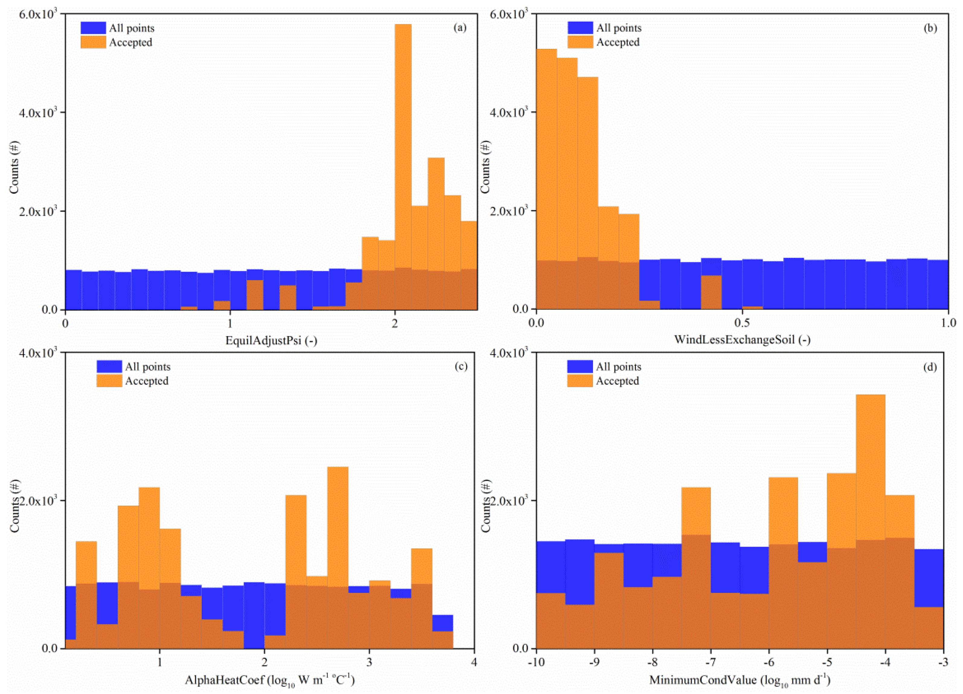
| EquilAdjustPsi | - | 0.00–2.50 | 2.06 | 0.69 | |
| MaxSoilCondens | mm·day−1 | 1.00–4.00 | 2.77 | 0.93 | |
| MaxSurfDeficit | mm | −4.00–0.00 | −2.42 | 0.96 | |
| MaxSurfExcess | mm | 0.00–3.00 | 1.22 | 0.96 | |
| RoughLBareSoilMom | m | 1.00 × 10⁻⁵–0.05 b | 4.26 × 10⁻³ | 0.96 | |
| WindLessExchangeSoil | - | 0.00–1.00 | 0.11 | 0.55 | |
| KBMinusOne | - | 0.00–2.50 | 1.32 | 0.96 | |
| Soil heat process | |||||
| AlphaHeatCoef | W·m−1·°C−1 | 0.01–5.00 × 10³ b | 483.33 | 0.82 | |
| FreezepointF1 | - | 0.00–2.00 | 0.94 | 0.98 | |
| FreezepointFWi | - | 0.01–1.00 | 0.52 | 0.99 | |
| TempDiffPrec_Air | °C | −5.00–5.00 | 0.23 | 0.99 | |
| CFrozenMaxDamp | - | 0.50–0.90 | 0.76 | 0.92 | |
| SandFrozenC4 | - | 0.01–1.00 | 0.54 | 0.96 | |
| SandUnfrozenC2 | - | 0.01–1.00 | 0.50 | 0.94 | |
| Soil water process | |||||
| DVapTortuosity | - | 0.01–2.00 | 0.97 | 0.99 | |
| InitialPressuredHead | cm | 1.00–200.00 | 119.91 | 0.99 | |
| MinimumCondValue | mm·day−1 | 1.0 × 10⁻¹⁰–1.0 × 10⁻³ b | 2.85 × 10⁻⁵ | 0.36 | |
| TempFacLinIncrease | °C−1 | 0.02–0.03 | 0.02 | 0.97 | |
| Depth (cm) | Soil Temperature | Total Water Content | ||||||
|---|---|---|---|---|---|---|---|---|
| Prior Range | Posterior Range | Prior Range | Posterior Range | |||||
| RLa | RHb | RL | RH | RL | RH | RL | RH | |
| R2 | ||||||||
| 5 | 0.7 | 1.0 | 0.9 | 1.0 | 0.0 | 0.7 | 0.4 | 0.7 |
| 15 | 0.7 | 1.0 | 0.9 | 1.0 | 0.0 | 0.9 | 0.4 | 0.9 |
| 25 | 0.7 | 1.0 | 0.9 | 1.0 | 0.0 | 0.9 | 0.4 | 0.9 |
| 35 | 0.7 | 1.0 | 0.9 | 1.0 | 0.0 | 0.8 | 0.4 | 0.8 |
| ME | ||||||||
| 5 | −6.0 | 8.7 | −1.5 | 2.2 | −34.4 | −2.0 | −10.1 | −2.0 |
| 15 | −5.3 | 8.2 | −1.3 | 2.1 | −30.0 | 3.6 | −7.4 | 0.9 |
| 25 | −5.1 | 7.4 | −1.3 | 1.8 | −31.0 | 4.1 | −7.7 | 0.9 |
| 35 | −4.6 | 6.9 | −1.1 | 1.7 | −30.2 | 1.5 | −7.5 | 0.4 |
| RMSE | ||||||||
| 5 | 1.6 | 10.4 | 1.6 | 3.8 | 7.1 | 36.5 | 7.1 | 14.4 |
| 15 | 1.0 | 9.2 | 1.1 | 3.1 | 3.4 | 31.1 | 3.6 | 10.4 |
| 25 | 0.9 | 8.2 | 0.9 | 2.7 | 3.6 | 31.9 | 3.6 | 10.6 |
| 35 | 0.7 | 7.7 | 0.7 | 2.4 | 3.0 | 30.8 | 3.0 | 10.0 |
| Variable/Depth | R2 | RMSE | ME | ||||||
|---|---|---|---|---|---|---|---|---|---|
| Pmean a | Smean b | Change | Pmean | Smean | Change | c Pwidth | d Swidth | Change | |
| Soil temperature | |||||||||
| 5 cm | 0.88 | 0.91 | 0.03 | 2.92 | 2.98 | 0.06 | 14.63 | 3.06 | −11.57 |
| 15 cm | 0.93 | 0.95 | 0.02 | 2.08 | 2.09 | 0.01 | 13.52 | 2.82 | −10.70 |
| 25 cm | 0.95 | 0.96 | 0.01 | 1.75 | 1.70 | −0.05 | 12.48 | 2.60 | −9.88 |
| 35 cm | 0.96 | 0.96 | 0.00 | 1.51 | 1.48 | −0.03 | 11.49 | 2.39 | −9.10 |
| Total water content | |||||||||
| 5 cm | 0.20 | 0.41 | 0.21 | 19.79 | 10.68 | −9.11 | 32.44 | 6.26 | −26.17 |
| 15 cm | 0.42 | 0.62 | 0.20 | 9.68 | 6.34 | −3.34 | 33.64 | 5.77 | −27.87 |
| 25 cm | 0.38 | 0.67 | 0.29 | 9.45 | 6.02 | −3.43 | 35.10 | 6.41 | −28.69 |
| 35 cm | 0.27 | 0.48 | 0.21 | 9.24 | 5.80 | −3.44 | 31.64 | 6.18 | −25.48 |
| Variable/Depth | R2 | RMSE | ME | |||
|---|---|---|---|---|---|---|
| SSmean a | Change | SSmean | Change | SSmean | Change | |
| Soil temperature | ||||||
| 5 cm | 0.92 | 0.01 | 2.37 | −0.60 | 0.95 | 0.35 |
| 15 cm | 0.96 | 0.01 | 1.74 | −0.36 | 1.13 | 0.49 |
| 25 cm | 0.95 | 0.00 | 1.66 | −0.05 | 0.94 | 0.62 |
| 35 cm | 0.95 | −0.02 | 1.72 | 0.24 | 1.06 | 0.75 |
| Total water content | ||||||
| 5 cm | 0.42 | 0.02 | 14.52 | 3.85 | −12.06 | −5.55 |
| 15 cm | 0.67 | 0.05 | 4.85 | −1.49 | −1.68 | 0.28 |
| 25 cm | 0.59 | −0.08 | 5.01 | −1.00 | −1.60 | 0.24 |
| 35 cm | 0.42 | −0.06 | 5.11 | −0.68 | −3.20 | 0.82 |
| Period | P+I | E | RO | ΔS | E/(P+I-ΔS) | RO/(P+I-ΔS) |
|---|---|---|---|---|---|---|
| mm | ||||||
| I | 14.83 | 53.42 | 4.83 | −43.42 | 0.92 | 0.08 |
| II | 259.40 | 29.66 | 114.31 | 115.43 | 0.21 | 0.79 |
| III | 0.00 | 1.17 | 32.88 | −34.05 | 0.03 | 0.97 |
| IV | 1.10 | 41.04 | 11.23 | −51.17 | 0.79 | 0.21 |
| V | 0.00 | 11.94 | 6.57 | −18.51 | 0.65 | 0.35 |
| Total | 275.33 | 137.23 | 169.87 | −31.77 | 0.45 | 0.55 |
| Output Variables | Unit | Parameter Set 1 | Parameter Set 2 | Parameter Set 3 |
|---|---|---|---|---|
| Total evaporation | mm | 157.92 | 63.77 | 88.98 |
| Total runoff | mm | 207.69 | 468.73 | 261.30 |
| Total latent heat | J·m−2 | 2.93 × 10⁸ | −1.49 × 10⁹ | −1.87 × 10⁹ |
| Total sensible heat | J·m−2 | 5.59 × 10⁸ | 2.66 × 10⁹ | 7.84 × 10⁹ |
© 2016 by the authors; licensee MDPI, Basel, Switzerland. This article is an open access article distributed under the terms and conditions of the Creative Commons by Attribution (CC-BY) license (http://creativecommons.org/licenses/by/4.0/).
Share and Cite
Wu, M.; Jansson, P.-E.; Tan, X.; Wu, J.; Huang, J. Constraining Parameter Uncertainty in Simulations of Water and Heat Dynamics in Seasonally Frozen Soil Using Limited Observed Data. Water 2016, 8, 64. https://doi.org/10.3390/w8020064
Wu M, Jansson P-E, Tan X, Wu J, Huang J. Constraining Parameter Uncertainty in Simulations of Water and Heat Dynamics in Seasonally Frozen Soil Using Limited Observed Data. Water. 2016; 8(2):64. https://doi.org/10.3390/w8020064
Chicago/Turabian StyleWu, Mousong, Per-Erik Jansson, Xiao Tan, Jingwei Wu, and Jiesheng Huang. 2016. "Constraining Parameter Uncertainty in Simulations of Water and Heat Dynamics in Seasonally Frozen Soil Using Limited Observed Data" Water 8, no. 2: 64. https://doi.org/10.3390/w8020064