Support Vector Regression for Rainfall-Runoff Modeling in Urban Drainage: A Comparison with the EPA’s Storm Water Management Model

Abstract

Rainfall-runoff models can be classified into three types: physically based models, conceptual models, and empirical models. In this latter class of models, the catchment is considered as a black box, without any reference to the internal processes that control the transformation of rainfall to runoff. In recent years, some models derived from studies on artificial intelligence have found increasing use. Among these, particular attention should be paid to Support Vector Machines (SVMs). This paper shows a comparative study of rainfall-runoff modeling between a SVM-based approach and the EPA’s Storm Water Management Model (SWMM). The SVM is applied in the variant called Support Vector regression (SVR). Two different experimental basins located in the north of Italy have been considered as case studies. Two criteria have been chosen to assess the consistency between the recorded and predicted flow rates: the root-mean square error (RMSE) and the coefficient of determination. The two models showed comparable performance. In particular, both models can properly model the hydrograph shape, the time to peak and the total runoff. The SVR algorithm tends to underestimate the peak discharge, while SWMM tends to overestimate it. SVR shows great potential for applications in the field of urban hydrology, but currently it also has significant limitations regarding the model calibration.

1. Introduction

An efficient drainage network aims to protect people and property within a catchment from harm [1,2]. The urban rainfall–runoff modeling is a long-debated question. The first hydrologists attempting to predict the flows that could be expected from a rainfall event also tried to understand hydrological processes, even if their methods were limited by computational techniques and available data. The first widely used rainfall-runoff model was the rational method, conceived by T. J. Mulvaney in 1850 [3]. Even if the model is a single equation, it manages to illustrate most of the problems that hydrological modelers have to address: Stormwater is generated by rainfall through a series of complex hydrological processes influenced by many variables. Rainfall-runoff transformation involves two main phases: Firstly, hydrological losses occur due to interception, depression storage, infiltration and evapo-transpiration; secondly, the resulting effective rainfall is transformed into an overland flow by surface routing. Finally, the surface flow is collected by the drainage system.

Stormwater drainage networks sizing is generally based on artificial peak events which are remote from real rainfall and runoff processes. Even Mulvaney warned about limitations of peak event-based approximations [4].

Existing hydrological models can be classified into three types, namely, (1) physically based models, (2) conceptual models, and (3) empirical models. The latter class of models, unlike the first two categories, involves mathematical equations that are derived from observations of the inputs to and outputs from a catchment basin: Rainfall–runoff modeling is carried out within a purely analytical framework based on time-series data. The catchment is considered as a black box, without any reference to the physical processes that control the transformation of rainfall to runoff. In recent years, some models derived from studies on artificial intelligence have found increasing use: artificial neural networks (ANNs) and Support Vector Machines (SVMs).

ANNs [5,6] aim to develop a predictive structure directly from the observational data. They are generally presented as a system of interconnected neurons that exchange information between each other, imitating the working of the brain. The simplest neural networks relate an input signal such as rainfall to an output signal such as runoff by means of a series of weighting functions that may involve a number of layers of interconnected nodes, including intermediate hidden layers. Several techniques are available for determining the appropriate model structure, which will be able to provide a framework for reflecting complexities and nonlinearities in the data as well as some characteristic processes for a particular catchment.

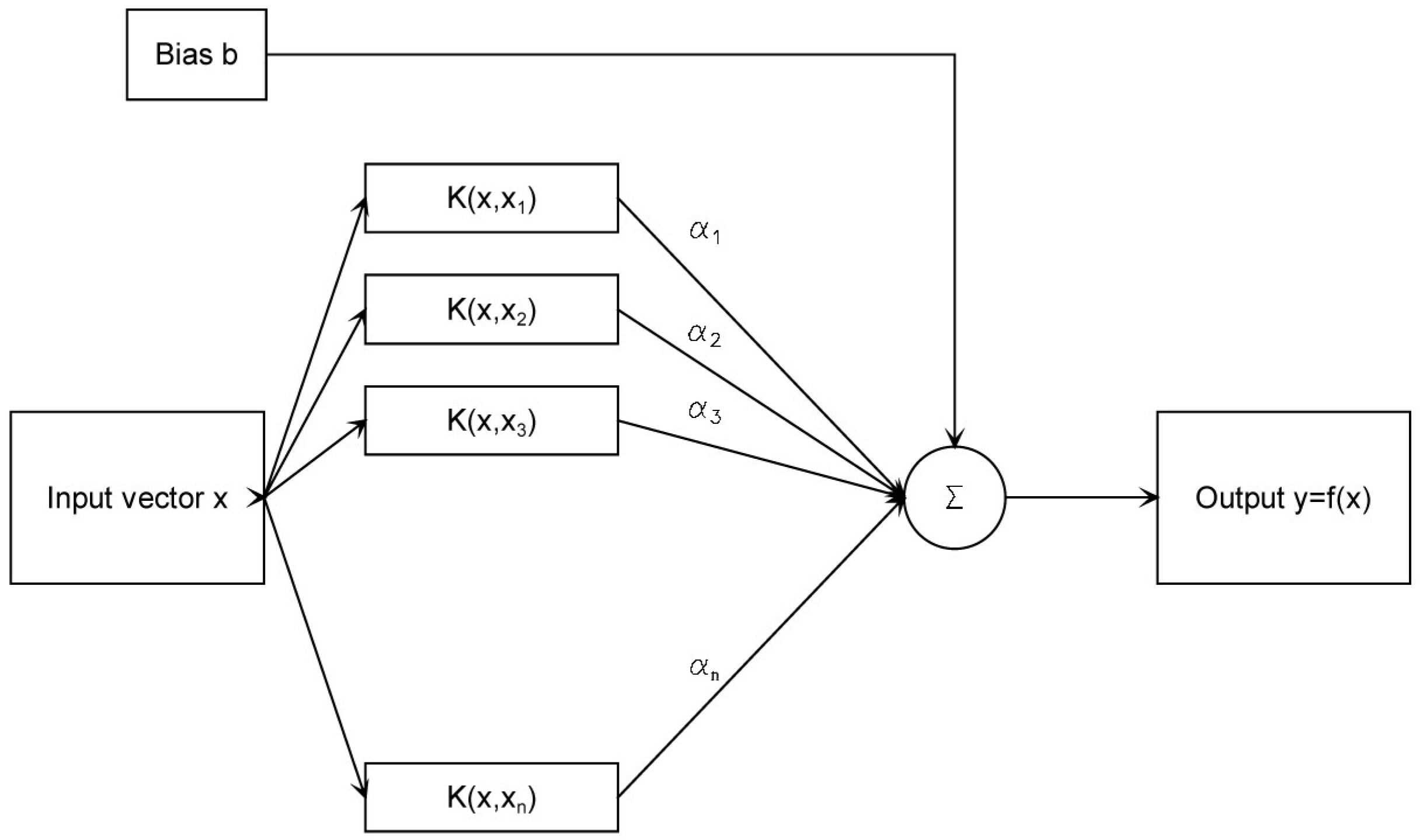
The SVMs [7,8] are machine-learning algorithms developed by Vapnik and other researchers [9,10,11]. This approach was also at first developed as a way of interpreting sensor data and it involves a two-layer structure. The first layer (Figure 1) is a nonlinear kernel weighting on the input variable series, the support vectors, and the second is a weighted sum of the kernel outputs. In many cases, SVMs may be more efficient than ANN methods, once the support vectors and appropriate kernel filters have been determined.

Many researchers have investigated the possibility of addressing hydrological problems using SVMs. Dibike et al. [12] investigated SVMs for rainfall-runoff modeling compared to ANN models. Bray and Han [13] highlighted the difficulties in identifying a suitable model structure and its relevant parameters for rainfall-runoff modeling. Tripathi et al. [14] showed an SVM approach for statistical the downscaling of precipitation at a monthly time scale. Chen et al. [15] used SVMs to predict daily precipitation in the Hanjiang basin. The SVM technique has also been successful recently in solving forestry problems [16], in determining the solar irradiation [17], in predicting the real-time flood [18], and in predicting the daily rainfall-runoff [19]. An extensive review of the SVM applications in the field of hydrology is provided by Raghavendra and Deka [20].

This paper shows a comparative study of rainfall-runoff modeling between a SVM-based approach and the well-known EPA’s Storm Water Management Model (SWMM). SVM is applied in the variant called Support Vector regression (SVR). Two different experimental basins located in the north of Italy have been considered as case studies. Actual observed rainfall and runoff data are used in the study.

2. Materials and Methods

2.1. Support Vector Regression

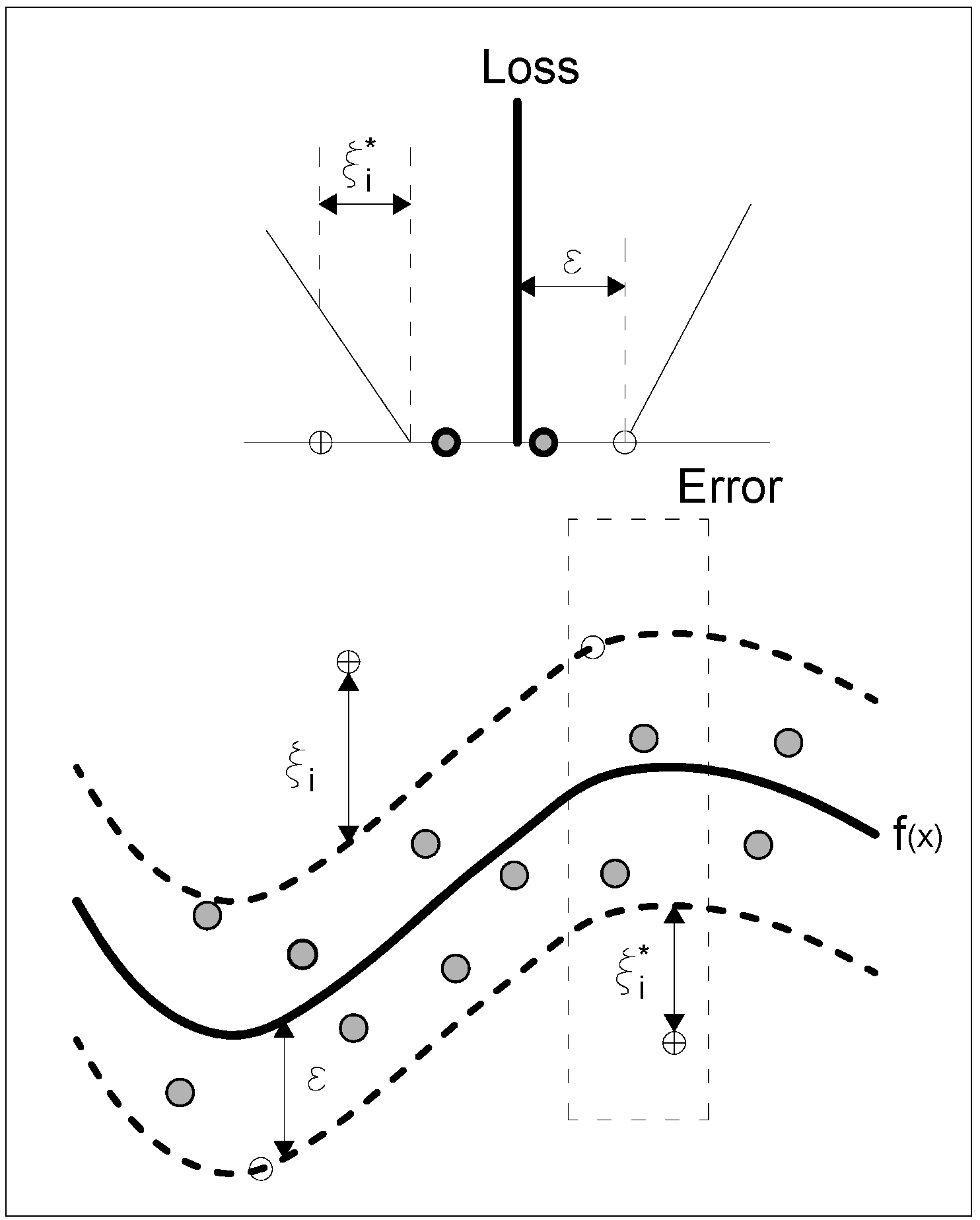
SVR fits a continuous-valued function to data (Figure 2) in a way that shares many of the advantages of SVM classification. Most algorithms for SVR [21,22] require that training samples are provided in a single batch. For applications such as on-line time-series prediction, a new model is required every time a new sample is added to (or removed from) the training set. Retraining for each new data point can be quite expensive.

The basic idea is the following: Given a training data set {(x₁, y₁), (x₂, y₂),…, (x_l, y_l)} ⊂ X × R, in SVR the goal is to find a function f(x) that has at most ε deviation from the actually obtained targets y_i for all the training data and, at the same time, is as flat as possible. The errors that are smaller than ε are not of concern, while the errors greater than ε are unacceptable. In the case of linear functions in the form

$$f(x)=\langle w,x\rangle +b$$

(1)

w ∈ X, b ∈ R, and the symbol $\langle \cdot ,\cdot \rangle$ denotes the dot product in X. In order to ensure this, the Euclidean norm ||w||² need to be minimized. Therefore, this problem can be seen as a convex optimization problem in the form

$$\text{minimize }\frac{1}{2}{\parallel w\parallel }^2.\text{subject to }\{\begin{array}{c}{y}_i-\langle w,x_i\rangle -b\le \epsilon \hfill \\ \langle w,x_i\rangle +b-y_i\le \epsilon \hfill \end{array}$$

(2)

Through Equation (2), it is implicitly assumed that there is a function f that approximates all the pairs (x_i, y_i) with ε precision. In cases where this is not possible, or a specified error can be tolerated, slack variables ζ_i, ζ_i^* can be introduced (Figure 2) in the otherwise infeasible constraints of the optimization problem, which can be stated according to the formulation:

$$\text{minimize }\frac{1}{2}{\parallel w\parallel }^2+C{\displaystyle \sum _{i=1}^l\left({\xi }_i+{\xi }_i^{*}\right)}\text{ subject to }\{\begin{array}{c}{y}_i-\langle w,x_i\rangle -b\le \epsilon +{\xi }_i\hfill \\ \langle w,x_i\rangle +b-y_i\le \epsilon +{\xi }_i^{*}\hfill \end{array}$$

(3)

The constant C > 0 directs the choice between the flatness of f and the amount up to which deviations larger than ε are tolerated. The optimization problem Equation (3) can be more easily solved in its dual formulation, utilizing Lagrange multipliers. The first step is to construct a Lagrange function from both the objective function and the constraints, introducing a dual set of variables:

$$L=\frac{1}{2}{\parallel w\parallel }^2+C{\displaystyle \sum _{i=1}^l\left({\xi }_i+{\xi }_i^{*}\right)-{\displaystyle \sum _{i=1}^l{\alpha }_{\mathrm{i}}\left(\epsilon +{\xi }_i-y_i+\langle w,x_i\rangle +b\right)-}}{\displaystyle \sum _{i=1}^l{\alpha }_i^{*}\left(\epsilon +{\xi }_i^{*}+y_i-\langle w,x_i\rangle -b\right)-}{\displaystyle \sum _{i=1}^l\left({\eta }_i{\xi }_i+{\eta }_i^{*}{\xi }_i^{*}\right)}$$

(4)

The dual variables in Equation (4) have to satisfy the conditions ${\alpha }_i,{\alpha }_i^{*},{\eta }_i,{\eta }_i^{*}\ge 0$, while the partial derivatives of L with respect to the primal variables $\left(w,\text{\hspace{0.17em}}b,{\xi }_i{\xi }_i^{*}\right)$ must vanish to reach the optimal condition:

$$\frac{\partial L}{\partial b}={\displaystyle \sum _{i=1}^l({\alpha }_i^{*}-{\alpha }_i)=0}$$

(5)

$$\frac{\partial L}{\partial w}=w-{\displaystyle \sum _{i=1}^l({\alpha }_i-{\alpha }_i^{*})x_i=0}$$

(6)

$$\frac{\partial L}{\partial {\xi }_i^{*}}=C-{\alpha }_i^{*}-{\eta }_i^{*}=0$$

(7)

Combining Equations (5)–(7) and Equation (4) leads to the dual optimization problem:

$$\text{maximize }\left\{\begin{array}{c}-\frac{1}{2}{\displaystyle \sum _{i,j=1}^l}({\alpha }_i-{\alpha }_i^{*})({\alpha }_j-{\alpha }_j^{*})\langle x_i,x_j\rangle \hfill \\ -\epsilon {\displaystyle \sum _{i=1}^l}({\alpha }_i+{\alpha }_i^{*})+{\displaystyle \sum _{i=1}^l}{y}_i({\alpha }_i-{\alpha }_j^{*})\hfill \end{array}\text{ subject to }\right\{\begin{array}{c}{\displaystyle \sum _{i=1}^l}({\alpha }_i-{\alpha }_i^{*})=0\\ {\alpha }_i,{\alpha }_i^{*}\in [0,C]\end{array}$$

(8)

The dual variables ${\eta }_i,{\eta }_i^{*}$ do not appear in the dual objective function because they have been eliminated through Equation (7). Equation (6) can be rewritten as:

$$w={\displaystyle \sum _{i=1}^l({\alpha }_i-{\alpha }_i^{*})x_i}$$

(9)

therefore,

$$f(x)={\displaystyle \sum _{i=1}^l\left({\alpha }_i-{\alpha }_i^{*}\right)}\langle x_i,x\rangle +b$$

(10)

which is the support vector expansion of the function f, while w can be completely expressed as a linear combination of the training patterns x_i.

The issue of computing b can be addressed by exploiting the Karush-Kuhn-Tucker conditions [23,24], which state that at the optimal solution the product between dual variables and constraints has to vanish, that is,

$$\begin{array}{l}{\alpha }_i\left(\epsilon +{\xi }_i-y_i+\langle w,x_i\rangle +b\right)=0\\ {\alpha }_i^{*}\left(\epsilon +{\xi }_i^{*}+y_i-\langle w,x_i\rangle -b\right)=0\end{array}$$

(11)

and

$$\begin{array}{l}(C-{\alpha }_i){\xi }_i=0\\ (C-{\alpha }_i^{*}){\xi }_i^{*}=0\end{array}$$

(12)

From that, some important considerations arise. First of all, only samples (x_i, y_i) with corresponding α_i^* = C are positioned outside the ε-insensitive tube around f. Secondly, α_iα_i^* = 0, that is a set of dual variables α_i, α_i^*, which are both simultaneously nonzero, does not exist. Finally, from α_i^*∈ (0, C) results ζ_i^* = 0, and the second factor in Equation (11) has to vanish. Therefore, b can be evaluated by the following:

$$\begin{array}{l}b=y_i-\langle w,x_i\rangle -\epsilon \\ b=y_i-\langle w,x_i\rangle +\epsilon \end{array}$$

(13)

for α_i ∈ (0, C) and α_i^* ∈ (0, C).

Subsequently, it is necessary to make the Support Vector algorithm nonlinear. This can be obtained by preprocessing the training patterns x_i by a map Φ: X→F, where F is some feature space [22]. The Support Vector algorithm only depends on dot products between the various patterns, so it is sufficient to know and use a kernel $k(x_i,x_j)=\langle \Phi (x_i),\Phi (x_j)\rangle$ instead of Φ(∙) explicitly. This allows us to rewrite the Support Vector algorithm as follows:

$$\text{maximize }\left\{\begin{array}{c}-\frac{1}{2}{\displaystyle \sum _{i,j=1}^l}({\alpha }_i-{\alpha }_i^{*})({\alpha }_j-{\alpha }_j^{*})k(x_i,x_j)\\ -\epsilon {\displaystyle \sum _{i=1}^l}({\alpha }_i+{\alpha }_i^{*})+{\displaystyle \sum _{i=1}^l}{y}_i({\alpha }_i-{\alpha }_j^{*})\end{array}\text{ subject to }\right\{\begin{array}{c}{\displaystyle \sum _{i=1}^l}({\alpha }_i-{\alpha }_i^{*})=0\\ {\alpha }_i,{\alpha }_i^{*}\in [0,C]\end{array}$$

(14)

The expansion of f can now be written as:

$$f(x)={\displaystyle \sum _{i=1}^l\left({\alpha }_i-{\alpha }_i^{*}\right)}k(x_i,x)+b$$

(15)

Unlike that in the linear case, w is no longer explicitly specified, though uniquely defined. In the nonlinear setting, the optimization problem corresponds to finding the flattest function in feature space, not in input space. The functions k(x_i, x_j) corresponding to a dot product in some feature space F have to satisfy the Mercer’s condition [22].

The kernel functions commonly used in SVR formulations are:

$$\text{Linear }k(x_i,x_j)=x_i^T{x}_j$$

(16)

$$\text{Polynomial }k(x_i,x_j)={(\gamma x_i^T{x}_j+r)}^d$$

(17)

$$\text{Radial basis function (RBF) }k(x_i,x_j)=\text{exp}\left(-\gamma {\parallel x_i-x_j\parallel }^2\right),\gamma >0$$

(18)

$$\text{Sigmoid }k(x_i,x_j)=\text{tanh}(\gamma x_i^T{x}_j+r)$$

(19)

A SVR algorithm has been implemented in a computer code written in MATLAB language. A radial basis function has been chosen as kernel. Input vectors contain rainfall and flow observations. However, as highlighted by Bray and Han [13], analysis results show that SVR effectiveness is less affected by rainfall and the performance enhancement of the model with increased flow observation is more significant than the improvement due to increased rainfall observation. An exhaustive search of an optimum model structure and its parameters is very complicated. It is based on a long and tedious trial and error iteration procedure, which is very difficult to automate and is omitted here for reasons of brevity. More details can be found in Bray and Han [13].

The deviation between the target value and the function found by the SVM is controlled by the ε parameter. In this study, ε has been finally chosen to be equal to 0.01, while the cost of error C, which is useful for controlling the smoothness of the function, has been assumed to equal 2.

2.2. SWMM

The well-known SWMM is a dynamic hydrology-hydraulic water quality simulation model. It is used throughout the world for analysis, design and planning related to stormwater runoff, combined and sanitary sewers, and other drainage systems. It can be used for single-event or long-term simulation [25] of runoff quantity and quality mainly from urban areas. The RUNOFF component operates on a collection of subcatchments that receive precipitation and generate runoff and pollutant loads. The ROUTING component transports this runoff through a system of pipes, channels, storage, treatment devices, pumps, and regulators.

The RUNOFF component generates hydrographs by processing rainfall data and a set of physical characteristics describing the catchment basin: area, slope, width, percent impervious, surface roughness, depression storage, and infiltration coefficients. The urban basin has to be divided into sub-basins with uniform characteristics. In order to model rainfall-runoff processes, each sub-basin is further divided into two parts: the pervious portion and the impervious portion. Each part is modeled as a nonlinear reservoir with a capacity given by the maximum depression storage. Infiltration is modeled by Horton’s equation, by Green-Ampt’s equation or by SCS Curve Number method.

The ROUTING component models the sewer system as a series of nodes and links. The nodes consist of manholes, storage units, flow dividers and outfalls, while the links consist of conduits, pumping systems, weirs, orifices and outlets. Surface runoff enters the sewer system at nodes. Runoff transport in sewer system is modeled by the classical De Saint-Venant equations.

Some parameters that characterize the hydrological behavior of the watershed are difficult to evaluate reliably; therefore, a calibration stage to estimate an optimal set of these parameters is essential. An automatic calibration technique has been used in this study. The technique is based on the optimization method called the complex method developed by Box [26]. The details of the procedure are shown in Barco et al. [27]. In this work, the following parameters have been considered in the calibration process: Manning’s coefficients, depression storage for both impervious and pervious area, and the parameters of the Green-Ampt’s equation (Suction Head S_u, Conductivity K_s and Initial Deficit). In order to simplify the calibration process, the width value for each sub-basin has been manually evaluated, in accordance with the suggestions of Rossman [25]. The constraints on the parameters were selected based on their physical meaning.

2.3. Case Studies

Two case studies [28] have been considered: the Merate experimental catchment and the Cascina Scala experimental catchment (Figure 3).

The Merate experimental catchment is located in the inner city of Merate, in the province of Lecco, 30 km far from Milan. The total area of the basin is 93.82 ha, 38% of which is impervious (19% roofs and 19% streets and paved surfaces). The entire basin is divided into three main sub-basins: A1, A2 and A3. The average slope of the basin is 2% in the north-south direction. The available experimental data refer to the sub-basin A2, which has an area of 20.83 ha, 20% of which is impervious. The basin has been subdivided in 76 subcatchments. The width of the subcatchments ranges from 31 m to 196 m.

The combined sewerage network in sub-basin A2 is made of 77 concrete conduits, and it has a total length of 1900 m. The diameters of the pipes range from 300 mm to 800 mm, while the slopes are all quite high. The rainfall on the basin is measured with three rain gauges. The temporal resolution is 2 min. In this study, 10 events recorded in Merate have been considered, 8 of which have been used for SVR algorithm training and 2 for testing.

The Cascina Scala experimental catchment is a residential district situated in Northern Pavia. The total area of the basin is 14.37 ha, while the contributing area is 11.35 ha, 65% of which is impervious (22.4% roofs and 42.5% streets and paved surfaces), and 35% is pervious. An area of 3.02 ha is not connected to the sewer system. The basin has been subdivided in 42 subcatchments. The width of the subcatchments ranges from 33 m to 201 m.

The combined sewerage network is made of 42 conduits and has a total length of 2045 m, while the slope of the sewer pipes ranges between 0.15% and 1.01%, with an average value weighted on the length of 0.42%. All the sewers are made of concrete pipes. The rainfall on the basin is measured by two rain gauges. The distance between the two rain gauges is 310 m; therefore, the spatial uniformity of the precipitation can be checked and the meteorological volume can be evaluated accurately. The temporal resolution is 2 min. In this research, 20 rainfall-runoff events recorded in Cascina Scala have been considered, 16 of which have been used for SVR training and 4 for testing.

Table 1. Calibrated parameters for SWMM simulations.

Basin:	MERATE
n IMP	n PERV	IMP D.S.	PERV D.S.	Su	Ks	i. m. d.
		(mm)	(mm)	(mm)	(mm/h)	(m/m)
0.13	0.45	1.1	5.5	120	5	0.2
Basin:	CASCINA SCALA
n IMP	n PERV	IMP D.S.	PERV D.S.	Su	Ks	i. m. d.
		(mm)	(mm)	(mm)	(mm/h)	(m/m)
0.014	0.4	1.25	2.46	150	7.4	0.15

summarizes the calibrated hydrologic parameters for the two basins.

3. Results and Discussion

Two criteria have been chosen to assess the consistency between the recorded and predicted flow rates: the root-mean square error (RMSE) and the coefficient of determination R². The latter is defined as

$$R^2=\left(1-\frac{{\displaystyle {\sum }_{i=1}^m{\left(Q_{pi}-Q_{mi}\right)}^2}}{{\displaystyle {\sum }_{i=1}^m{\left(Q_a-Q_{mi}\right)}^2}}\right)$$

(20)

where m is the total number of measured data, Q_pi is the predicted discharge for data point i, Q_mi is the measured discharge for data point i, and Q_a is the averaged value of the measured discharges.

In

Table 2. Simulation results.

Basin	Event [28]	Total Rainfall	Qmax (m3/s)			tpeak			Total Runoff (mm)			RMSE (m3/s)		R2
		(mm)	Obs.	SVR	SWMM	Obs.	SVR	SWMM	Obs.	SVR	SWMM	SVR	SWMM	SVR	SWMM
Merate	718	13.80	0.614	0.548	0.653	76'	74'	74'	4.23	4.51	4.73	0.0187	0.0282	0.984	0.963
	730	18.40	0.263	0.230	0.301	334'	338'	332'	7.77	7.89	8.18	0.0115	0.0183	0.971	0.926
Cascina Scala	402	13.55	0.140	0.136	0.135	94'	98'	94'	7.49	7.70	7.47	0.0076	0.0911	0.969	0.964
	418	25.96	0.319	0.294	0.381	38'	40'	40'	10.78	10.75	11.6	0.0097	0.0298	0.986	0.868
	419	7.80	0.270	0.236	0.312	20'	22'	18'	2.43	2.67	2.90	0.0128	0.0283	0.964	0.823
	430	5.99	0.071	0.066	0.070	54'	62'	50'	1.26	1.91	1.94	0.0079	0.0105	0.751	0.567

, the rainfall-runoff events considered for the two basins and the results of the simulations are reported.

Table 3. Relative errors of peak discharge and total runoff.

Basin	Event	Rainfall	Qmax Error (%)		Runoff Error (%)
		(mm)	SVR	SWMM	SVR	SWMM
Merate	718	13.80	−10.7	6.4	6.6	11.8
	730	18.40	−12.5	14.4	1.5	5.2
Cascina Scala	402	13.55	−3.3	−3.7	2.8	−0.3
	418	25.96	−7.8	19.4	−0.3	7.9
	419	7.80	−12.8	15.4	9.9	19.6
	430	5.99	−6.2	−1.7	51.6	54.0

shows the errors in the estimate of peak discharge and total runoff.

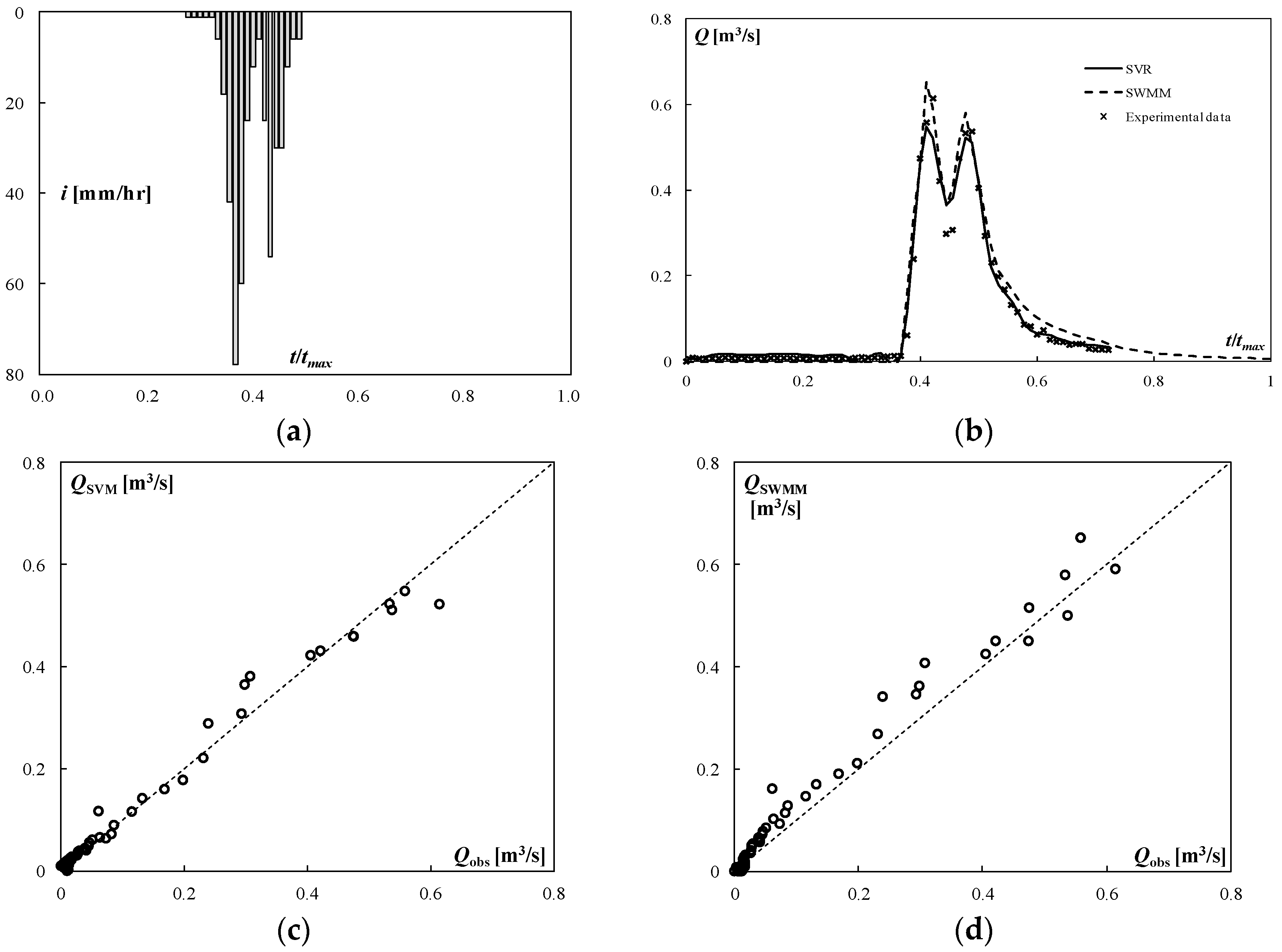
As for the Merate basin, in the simulation of Event 718, the algorithm SVR leads to an underestimation of the peak discharge of about 11%, while SWMM leads to an overestimation of about 6%. Both models predict the peak time with a slight advance (2 min). Moreover, both models overestimate the total runoff. The SVR model shows lower RMSE and a greater coefficient of determination: It provides a better prediction of flow, as also shown from the flood hydrograph (Figure 4). However, SWMM ensures a margin of safety in peak discharge prediction. Event 718 is characterized by a rainfall intensity that reached almost 80 mm/h and a peak flow rate of 0.614 m³/s.

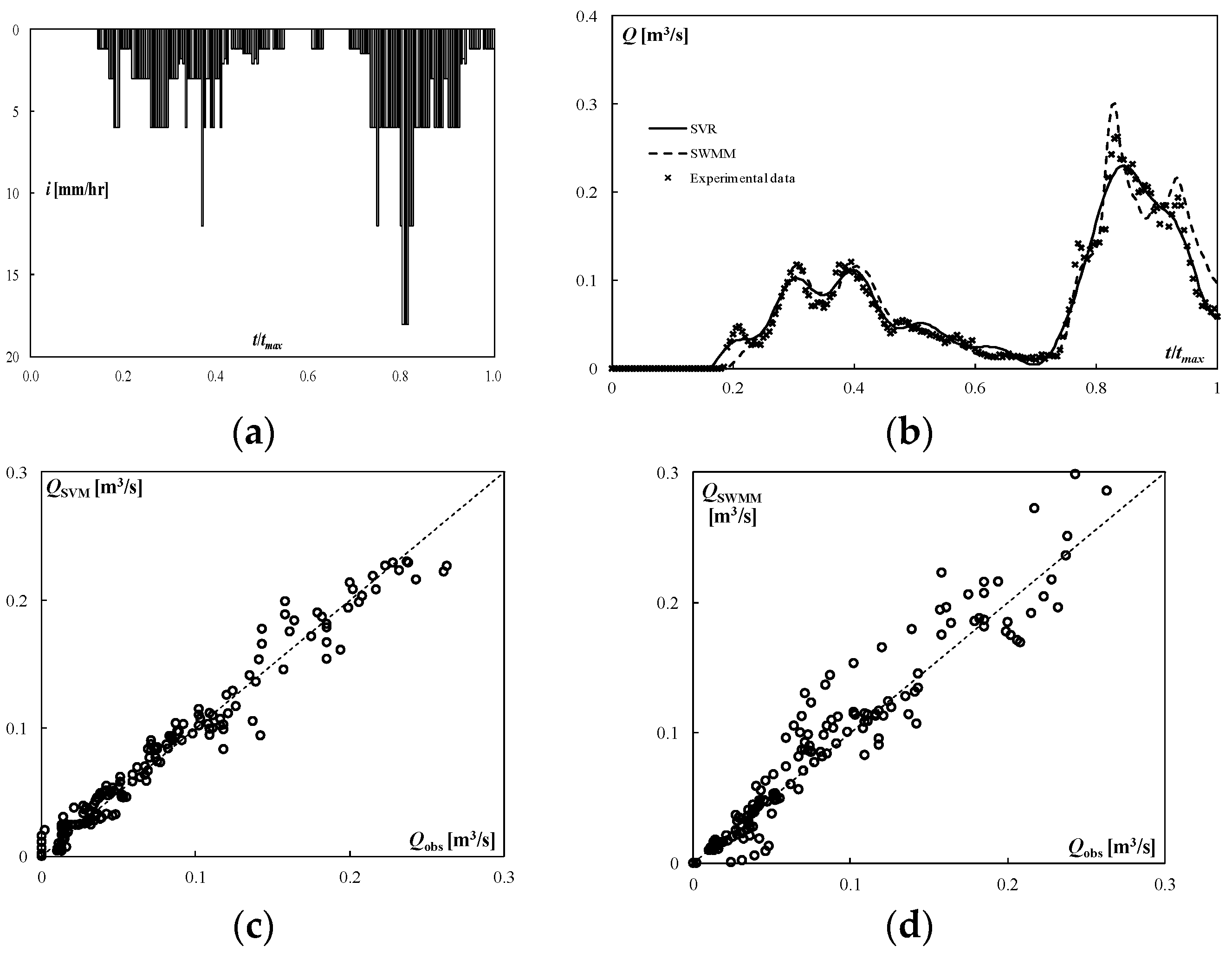
In simulating Event 730, the SVR leads to an underestimation of the peak discharge of about 13%, while SWMM leads to an overestimation of about 14%. SVR predicts the peak time with a delay of 4 min, while SWMM predicts the peak time with an advance of 2 min.

Both models, again, lead to an overestimation of the total runoff. The SVR shows a lower RMSE and a higher coefficient of determination, but both models are able to reproduce quite well a varied hydrograph (Figure 5). Event 730 was characterized by a rainfall intensity that did not exceed 20 mm/h and a long duration (about 6 h and 40 min).

Regarding the Cascina Scala basin, in the simulation of Event 402, both models provide a slight underestimation of the peak discharge (the error is 3.3% for SVR and 3.7% for SWMM). The peak time is predicted with a delay of 4 min by SVR, while it is predicted with great accuracy by SWMM. Even the total runoff is well predicted by SWMM, while SVR leads to a slight overestimation. Once again, SVR predictions are characterized by lower RMSE and a greater coefficient of determination. Additionally, in this case both models can reproduce the flood hydrograph quite well (Figure 6), except at the beginning, where the SVR algorithm unreasonably provides flow rates other than zero.

As for Event 418, SVR leads to an underestimation of the peak discharge of 7.8%, while the SWMM model provides an overestimation of almost 20%. Both models forecast the peak time with a delay of 2 min. The SVR algorithm well predicts the total runoff, while SWMM leads to a slight overestimation. The better accuracy of SVR is certified also in this case by RMSE and CE.

In simulating Event 419 SVR provides an appreciable underestimation of the peak flow rate (−12.8%), while SWMM provides a somewhat higher result than the experimental one (+15.4%). The peak time is predicted with a delay of 2 min by SVR, while it is predicted with an advance of 2 min by SWMM. Both models provide a considerable overestimation of the total runoff (+9.9% SVR, +19.6% SWMM), while SVR shows lower RMSE and a greater coefficient of determination.

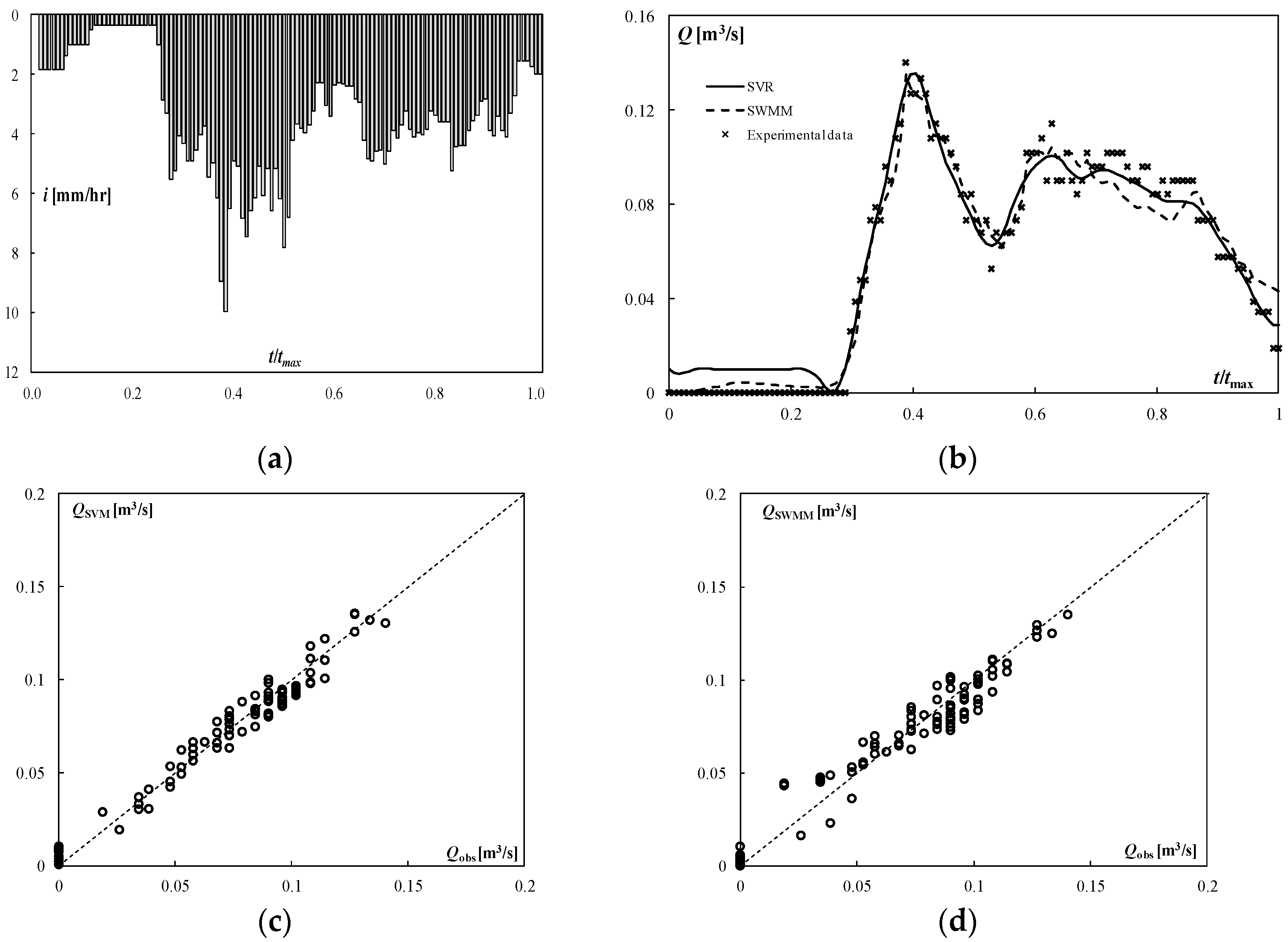
Finally, in simulating Event 430 both models produce less satisfactory results than in the other events.

Even if the errors on the peak flow rate and on time to peak are small, the error on the total runoff exceeds 50% for both SVR and SWMM. Both models fail to adequately simulate the second part of the hydrograph (Figure 7). Obviously, the RMSE and the coefficient of determination certify in a clear manner the smaller accuracy of the results. The reason why both models show poor performance in this case is not easy to understand. Probably the hyetograph, which is significantly different from those used in the calibration procedures, is the main cause of the unsatisfactory results. In this hyetograph, the highest rainfall intensity is observed for t/t_max < 0.2. For t/t_max > 0.2 rainfall intensity is reduced, except for a short time interval around t/t_max = 0.5. None of the events that have been considered in the calibration process has similar characteristics. Being a non-physically based method, SVR may lead to unexpected results in some cases.

In the simulation of the considered rainfall events, therefore, the SVR algorithm and SWMM show comparable performance in modeling a rainfall-runoff process in an urban basin. SVR shows a tendency to underestimate the peak discharge, thus providing results that may be inadequate in problems of verification of existing sewers. However, it can effectively represent the hydrograph shape, as well as the total runoff.

In future developments of this study it will be interesting to investigate how the SVR method may cope with volume driven processes. Currently, it is difficult to say whether SVR can properly cope with continuous sequences of rainfall in contrast to single events. In any case, the effectiveness of the method will depend on the structure of the input vectors and on the availability and quality of data for the training process.

4. Conclusions

An approach based on SVR has been used in the simulation of rainfall-runoff processes in two experimental basins located in Northern Italy. The same events have been simulated by the EPA’s Storm Water Management Model. The two models show comparable performance. Both models can properly model the hydrograph shape and the time to peak. In the simulated events, the results of SVR were characterized by higher values of the coefficient of determination and by lower RMSEs compared to the results of SWMM. In addition, the SVR algorithm tends to underestimate the peak discharge, up to over 10%, while SWMM tends to overestimate peak flow rate, up to 20%. Both models generally tend to overestimate the total runoff: SVR provides slightly better results once again. Nevertheless, SVR may lead to unexpected results in practical applications, being a non-physically based method.

SVR shows considerable potential for applications to the problems of urban hydrology. However, it is necessary to work hard to overcome the current limitations of this approach. It is essential to try to automate the identification of a suitable kernel function and of the main features of the model. Therefore, it appears appropriate that a similar approach is tested on a large number of case studies.