Objective Classification of Rainfall in Northern Europe for Online Operation of Urban Water Systems Based on Clustering Techniques

Abstract

This study evaluated methods for automated classification of rain events into groups of “high” and “low” spatial and temporal variability in offline and online situations. The applied classification techniques are fast and based on rainfall data only, and can thus be applied by, e.g., water system operators to change modes of control of their facilities. A k-means clustering technique was applied to group events retrospectively and was able to distinguish events with clearly different temporal and spatial correlation properties. For online applications, techniques based on k-means clustering and quadratic discriminant analysis both provided a fast and reliable identification of rain events of “high” variability, while the k-means provided the smallest number of rain events falsely identified as being of “high” variability (false hits). A simple classification method based on a threshold for the observed rainfall intensity yielded a large number of false hits and was thus outperformed by the other two methods.

1. Introduction

Rainfall is an important boundary condition for the design and operation of urban drainage systems. Compared to natural hydrology, detailed knowledge of the rainfall processes is even more important in the urban context as a result of the short reaction times from rainfall to runoff and the small spatial scales involved. From the view of a (urban) water systems operator, rain events can mainly be distinguished into two classes, stratiform and convective, which pose distinctly different challenges to the water system. Stratiform events typically cover large areas and are relatively continuous and uniform in intensity, while locally confined, vertical atmospheric motions characterize convective events [1], which often result in high rain intensities and large spatial variability. For a number of reasons we are interested in classifying rain events into these two classes based on available observations. In a design context, this could be choosing rain events as input for simulation studies, where the performance of different water system designs is evaluated in different situations [2]. For online purposes, we might want to apply a classification as input to a forecasting system which allows operators to, for example, avoid overloading the capacity of the sewer system by optimizing the operation of pumping stations or other actuators. In such forecasting applications radar rainfall measurements could be processed differently for different event types [3,4], different flow forecast models could be applied [5], or the uncertainty scaling of a probabilistic flow forecast could be changed [6]. In the case of online classification it is typically important to provide a reliable identification of convective events as soon as possible during an event.

Classification of weather types can be performed subjectively or objectively. An overview of classification approaches is provided in [7,8]. Most approaches focus on large scales and apply additional input data such as atmospheric pressures, which may be unnecessary to distinguish rain events with stratiform and convective characteristics and which may be hard to obtain for operators of drainage systems. Simpler methods have applied thresholds for the observed rain intensity [9,10] or thresholds on mean rain intensity in the neighbourhood of a point [11], but may not fully exploit spatial and temporal patterns present in the data. Integer valued time series models have previously shown promising results for distinguishing between convective and stratiform rain events using rain gauge observations [12]. However, such techniques were developed for simple point measurements and become challenging on large datasets, both in terms of the analytical and the computational effort required.

During recent years, significant progress was made in measuring and forecasting spatial rainfall fields through radar [3,13,14,15,16,17], as well as numerical weather predictions (NWP) [14,18] for operational and design purposes in urban hydrology and future developments may lead to the application of satellite observations [19]. The spatial information in such data can be exploited for the purpose of distinguishing between different types of rainfall events [20]. Spatial rainfall information is provided over a variety of scales, ranging from countrywide radar or rainfall forecast products [3,21] to local area weather radar installations, covering areas in the range of 100 km² [22,23].

The aim of this study was to evaluate whether clustering and Gaussian techniques can be applied for the purpose of classifying types of rainfall events in online and offline situations based on rainfall observations only. Such techniques are easier to apply and easier to scale than previously applied modelling techniques [12]. At the same time, they allow for the exploitation of spatial and temporal features in rainfall measurements and forecasts, which should lead to higher classification accuracy than the application of simple threshold methods. Researchers [24] have suggested such a feature-based classification method for mesoscale data, but did not evaluate the applicability of their approach for detection during an event. The techniques applied in this article were developed for a set of rain gauge measurements with high temporal and spatial resolution, but should be applicable to large datasets of radar rainfall measurements or numerical weather predictions (NWP) with minor modifications.

In the following, the article is divided into two parts. First, a scheme for objective classification of rain events in offline situations was developed and applied to a set of historical measurements. Subsequently, methods for classifying rain events in an online situation were tested. In this second part, the classification obtained in the offline setting was used as a reference and the aim was to identify rain events of high spatial and/or temporal variability (i.e., convective events) as soon as possible after the beginning of the event, without falsely classifying stratiform events as being convective.

2. Materials and Methods

2.1. Rain Gauge Dataset

We used rain gauge observations from 34 gauges in the Copenhagen area (Figure 1). The gauges are operated by the Danish Water Pollution Committee (SVK) [25]. The considered dataset ranges from January 2009 until September 2015. The data were available with a temporal resolution of 1 min. We decided to integrate the measurements to a resolution of 10 min. The reasoning behind this was that the classification methodology proposed here might, with some modifications, also be applicable to radar rainfall data or numerical weather predictions which are often available at a temporal resolution of 10 min.

We identified rain events based on the common dataset of measurements for all gauges. A rain event was defined as starting if the measured intensity at one of the considered gauges exceeded the threshold level of 0.02 mm/min [26]. A rain event was defined as ending if the measured rain intensity at all gauges had, for at least one hour, been lower than the threshold level. The data in this separation period of one hour were not considered in the further analysis. Only rain events with a minimum length of 3 time steps or 30 min duration were considered in the analysis. In total, 1538 events were identified.

We split the dataset into a calibration period from January 2009 to March 2011, containing 454 rain events, and a validation period from March 2011 to September 2015, containing 1084 rain events.

2.2. Clustering for Event Type Identification Offline Based on Spatial and Temporal Characteristics

As a first step, we aimed to classify all 454 rain events in the calibration period as being either convective or stratiform. The classification developed for the calibration period was subsequently applied for the validation period and formed the reference for the online classification approaches. As the applied classification approach was purely data-driven and not verified against an expert classification, we denoted the groups as rain events of “high” and “low” variability to emphasize that our clustering may not fully correspond to a meteorological definition of stratiform and convective event types.

A common method for identifying groups in a dataset is k-means clustering. This technique was applied for the classification of extreme events in [27]. The application of a clustering methodology requires the definition of properties that can be used to characterize the rain events. Subsequently, the clustering algorithm can be used to sort the events into groups. These steps are described in the following sections.

2.2.1. Defining Features to Characterize Rain Events

Stratiform and convective rain events should have clearly different characteristics in terms of rain intensity as well as spatial and temporal variability. Convective events are often characterized by high rain intensities that can vary strongly in space and time, because the associated storms often travel at high velocities and are of limited extent. Stratiform events, on the other hand, would typically be more widespread with long-lasting rainfall over extended areas. Based on aggregated values for whole rain events, we investigated a number of features that may describe these characteristics in the dataset of rain gauge observations. We considered:

• criteria focusing on the maximal observed rain intensity:

  • mean rain intensity during an event averaged over all gauges (MAVINT),
  • maximum rain intensity observed at any gauge during an event (MAXRMAX),
• criteria focusing on the spatial variation of the observed rainfall:

  • spatial variation of the mean rain intensities observed at the different gauges during an event, expressed as standard deviation of the mean rain intensities (SDAVINT),
  • spatial variation of the maximal rain intensities observed at the different gauges during an event, expressed as standard deviation of the maximal rain intensities (SDRMAX),
  • spatial variation of the instantaneous rain intensities observed at the different gauges, expressed as standard deviation of rain intensities measured at all gauges in the same time step, averaged over the whole event (SPATSD),
  • percentage of time steps without rain during a rain event, averaged over all rain gauges (MNLEN), and
• criteria focusing on the temporal variation of observations during an event:

  • absolute difference between measurements for consecutive time steps, averaged over all time steps and then all gauges. Only non-zero observations were considered. This property describes the degree of variation from one time step to another (MDEV).

The MNLEN feature may be considered a measure of spatial and temporal variability. If a rain event is highly variable and does not cover the whole considered area, it will occur time-lagged at the different gauges and in some places will not occur at all. This means that many of the gauges should exhibit a large percentage of zero observations in the course of the event.

After the computation of the above features, they were standardized to a mean of zero and a standard deviation of one. The correlation between the features was evaluated for the whole set of rain events described in Section 2.1. The resulting correlation matrix is depicted in

Table 1. Correlation between features used for characterizing variability of rain events.

Feature	MAVINT	SDAVINT	SPATSD	MAXRMAX	SDRMAX	MNLEN	MDEV
MAVINT	1.00	0.90	0.87	0.77	0.78	0.26	0.76
SDAVINT	0.90	1.00	0.76	0.63	0.73	0.41	0.57
SPATSD	0.87	0.76	1.00	0.89	0.89	0.11	0.88
MAXRMAX	0.77	0.63	0.89	1.00	0.96	0.09	0.85
SDRMAX	0.78	0.73	0.90	0.96	1.00	0.18	0.78
MNLEN	0.26	0.41	0.11	0.09	0.18	1.00	−0.01
MDEV	0.76	0.57	0.88	0.85	0.78	−0.01	1.00

. Clearly, many of the above features were strongly correlated (Table 1). We therefore applied principal component analysis (PCA, [28]) to identify a reduced set of variables which were independent from each other and could be used as input for a clustering routine (Section 2.2.2). The first 3 principal components were applied for classification in this study (Section 3).

2.2.2. Clustering into Event Types

A common method to identify groups in a dataset is k-means clustering. We have applied the algorithm by [29], which is implemented in the R-package “Vegan” [30]. For a given number of clusters $K$, the algorithm identifies the location of the cluster centres in such a way, that the overall sum of squares from the data points to the nearest cluster centre is minimized. In the setup considered here, a data point corresponds to a vector of standardized properties, characterizing spatial and temporal variability for a rain event as described in the previous section.

The approach requires the user to define a number of clusters $K$ which should be considered. This number should be small enough to yield stable and interpretable results for the clustering step. At the same time, $K$ should be large enough to be able to describe the major variations in the dataset. The following criterion was used to identify the optimal number of clusters [31]:

$$CH=\frac{SSB/K-1}{SSW/n-K}$$

(1)

In Equation (1), $SSW$ corresponds to the sum of squares within the clusters, i.e., the sum of squared distances between the data points and the centre of the cluster assigned to each data point. SSB corresponds to the sum of squares between the clusters, i.e., the sum of squared distances between all the cluster centres. $K$ is the number of clusters considered and $n=454$ is the number of data points (or rain events) in the calibration period. The optimal number of clusters maximizes the criterion $CH$. The maximum is obtained by defining as few clusters as possible, that should have a distance $SSB$ as far as possible from each other, and by minimizing the distance $SSW$ between the data points and the corresponding cluster centre.

After identifying $K=5$ as a suitable number of clusters and grouping all 454 rain events into clusters, the clusters were manually classified as events with “high” and “low” variability, based on the location of the cluster centre (see Section 3).

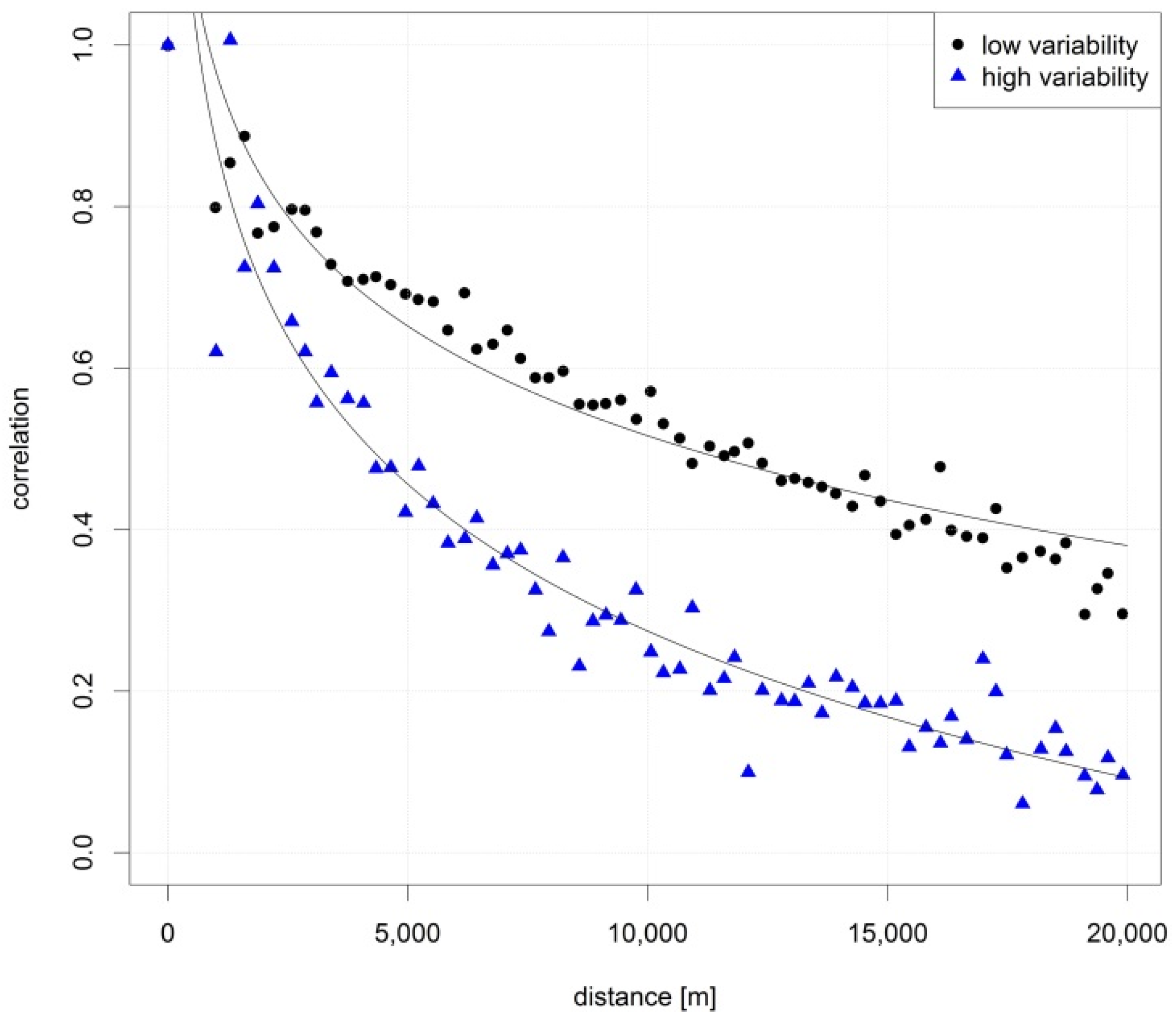
2.2.3. Validating Spatial and Temporal Variability of the Identified Groups of Rain Events

As a result of the approach described in the previous sections, all rain events in the calibration period were classified as being either of type “high” variability or of type “low” variability (i.e., convective or stratiform). However, the proposed methodology for offline classification is purely data-driven and based on a number of criteria that were solely defined based on common sense. The result of the classification should therefore be validated by analyzing the spatial and temporal characteristics of the identified groups in more detail, and by verifying that the events identified as being of “high” variability actually exhibit characteristics which are distinctly different from those events classified as being of “low” variability.

For the verification procedure, the dataset of 10 minute rainfall observations was split into two parts, each containing only those rain events that were classified as being of “high” and “low” variability, respectively.

Subsequently, covariograms [32] were computed for the two groups to describe the degree of similarity of rainfall measurements obtained at equal time points in space. The correlation between distant rainfall measurements would be expected to be much smaller for rain events that were classified as being of “high” variability, than for those of “low” variability.

The degree of similarity between rainfall measurements obtained at the same location but different time points can be described by the autocorrelation (ACF) and partial autocorrelation (PACF) functions [33]. These were computed separately for each rain event at each rain gauge, and subsequently averaged over all rain events. The median as well as the 2.5% and 97.5% quantiles of the ACF and PACF values obtained for the different locations and time lags are presented in Section 3.

2.3. Identifying Event Types Online in the Course of a Rain Event

While the previous sections focused on classifying rain events in an offline setting after the end of an event, the second part of the article focuses on classifying events in an online setting. The purpose of this work was to reliably identify rain events of “high” variability as soon as possible after the beginning of the event, while grouping as few as possible events of “low” variability falsely into the group of “high” variability (“false hits”).

The calibration period was used for training the online classification methods based on the results obtained in the offline classification. In the validation period, the classification results obtained using the online classification approaches were compared to the “truth” derived by classifying the rain events in the validation period using the off-line classification approach derived in the calibration period.

Four methods were tested to classify rain events online:

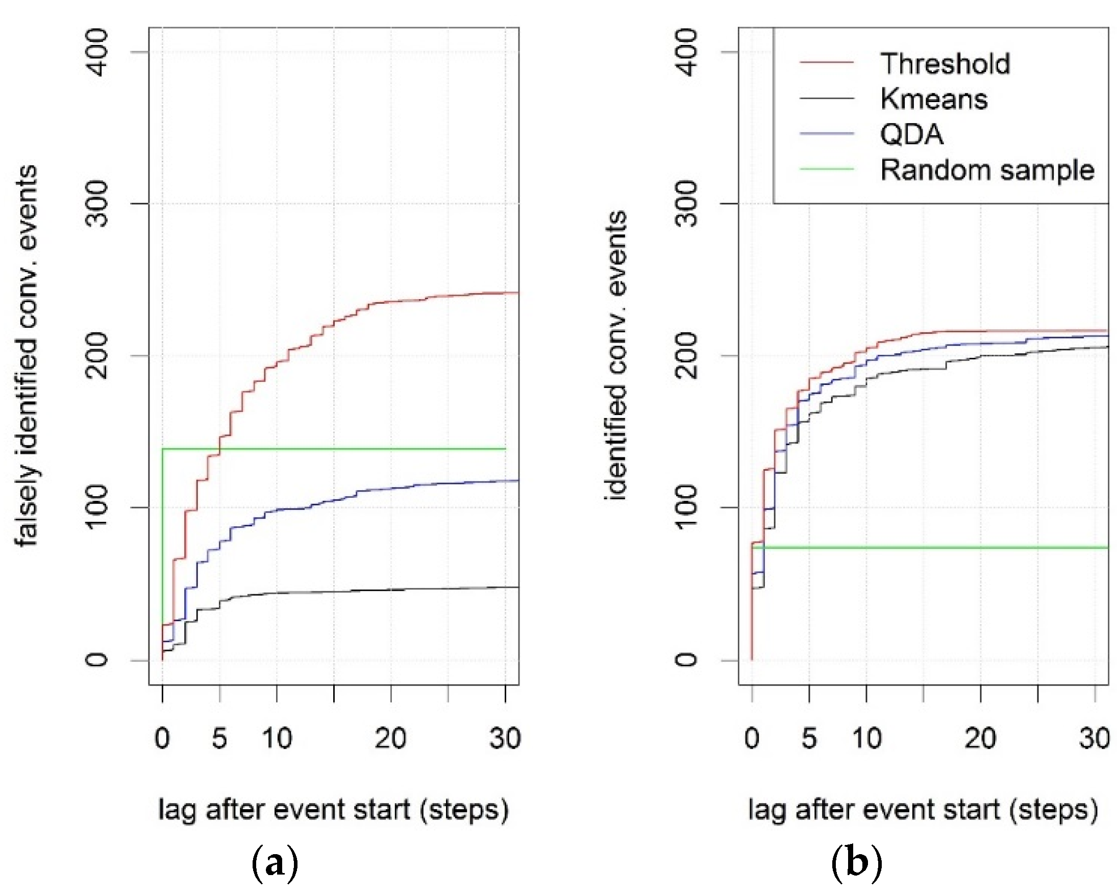
• Threshold on the observed rain intensity—A rain event was classified as convective if the 10-min rain intensity exceeded a threshold of 5.0 mm/h. The threshold was tuned manually during the calibration period to yield a high number of correctly identified convective events and a low number of false hits and was similarly applied in other studies [9].
• K-means clustering—The variables used for grouping rain events into clusters offline (Section 2.2 and Section 3) were computed recursively during a rain event, whenever new observations became available. Using the loadings derived from principal component analysis in the offline situation, the variables were transformed into the same first three principal components that were used offline. Based on the computed features, the nearest cluster centre defined during offline classification was identified. If the corresponding cluster was considered a cluster of events with “high” variability, the rain event would be classified as being of “high” variability.
• Quadratic discriminant analysis (QDA) [28]—Principal components were computed recursively in the same way as described for the clustering procedure in point 2 above. This recursive computation was performed during both calibration and validation periods. The discriminant model was trained during the calibration period based on the clusters derived during offline classification (Section 3). For each of the clusters identified offline, the mean and the variance of the three principal components were computed and used to define a separate multivariate normal distribution for each cluster. After training the discriminant model during the calibration period, it was applied to the validation period. Here, the discriminant model would compute the likelihood (probability density) for each newly obtained value to be a member of each cluster. The value was then classified into the cluster which scored the highest likelihood [28].
• Random sampling—This is a benchmark where an event is randomly classified based on the percentages of events of “high” and “low” variability identified during offline classification for the calibration period. As convective events are unlikely to occur during winter, we distinguished between summer and winter periods. 29.2% of the rain events were convective in the period from 1 May until 31 October, and 2.7% during the winter months.

3. Results and Discussion

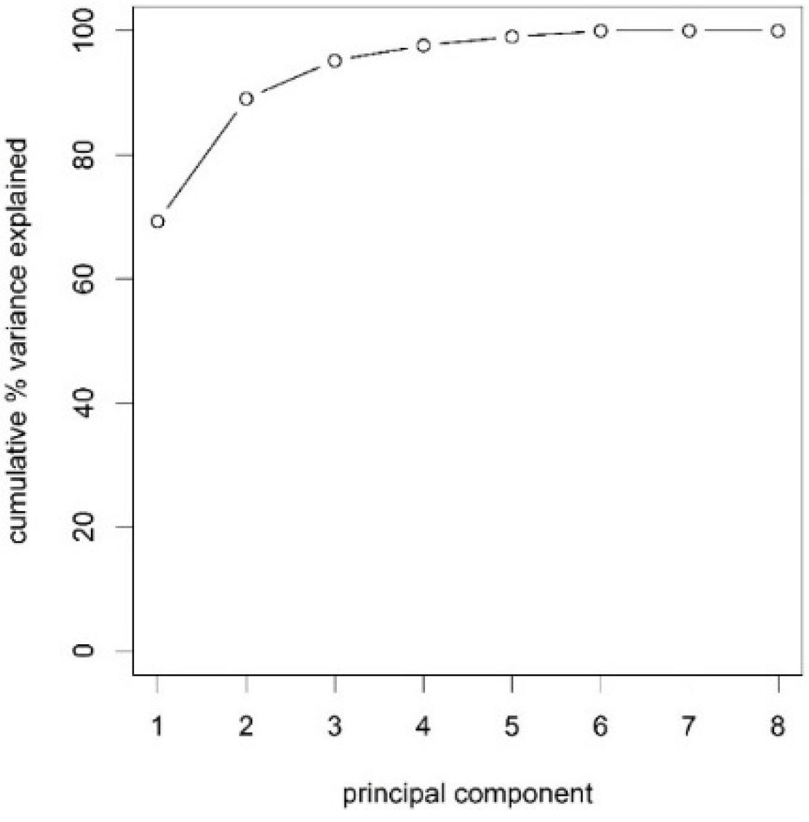
3.1. Reduction of Identification Variables Using Principal Component Analysis

We applied PCA to the set of standardized identification variables computed for offline classification as described in Section 2. The result showed that the first three principal components captured approximately 95% of the total variance present in the dataset (Figure 2). We therefore chose to subsequently describe the variability of the rainfall measurements using the first three principal components. These were obtained as a linear combination of the original variables using the loadings shown in

Table 2. Loadings for the identification variables in the first three principal components.

Principal Component	MAVINT	SDAVINT	SPATSD	MAXRMAX	SDRMAX	MNLEN	MDEV
Component 1	−0.412	−0.376	−0.427	−0.411	−0.420	−0.105	−0.388
Component 2	0.111	0.323	−0.123	−0.187	–	0.866	−0.285
Component 3	0.442	0.574	–	−0.398	−0.321	−0.426	−0.175

.

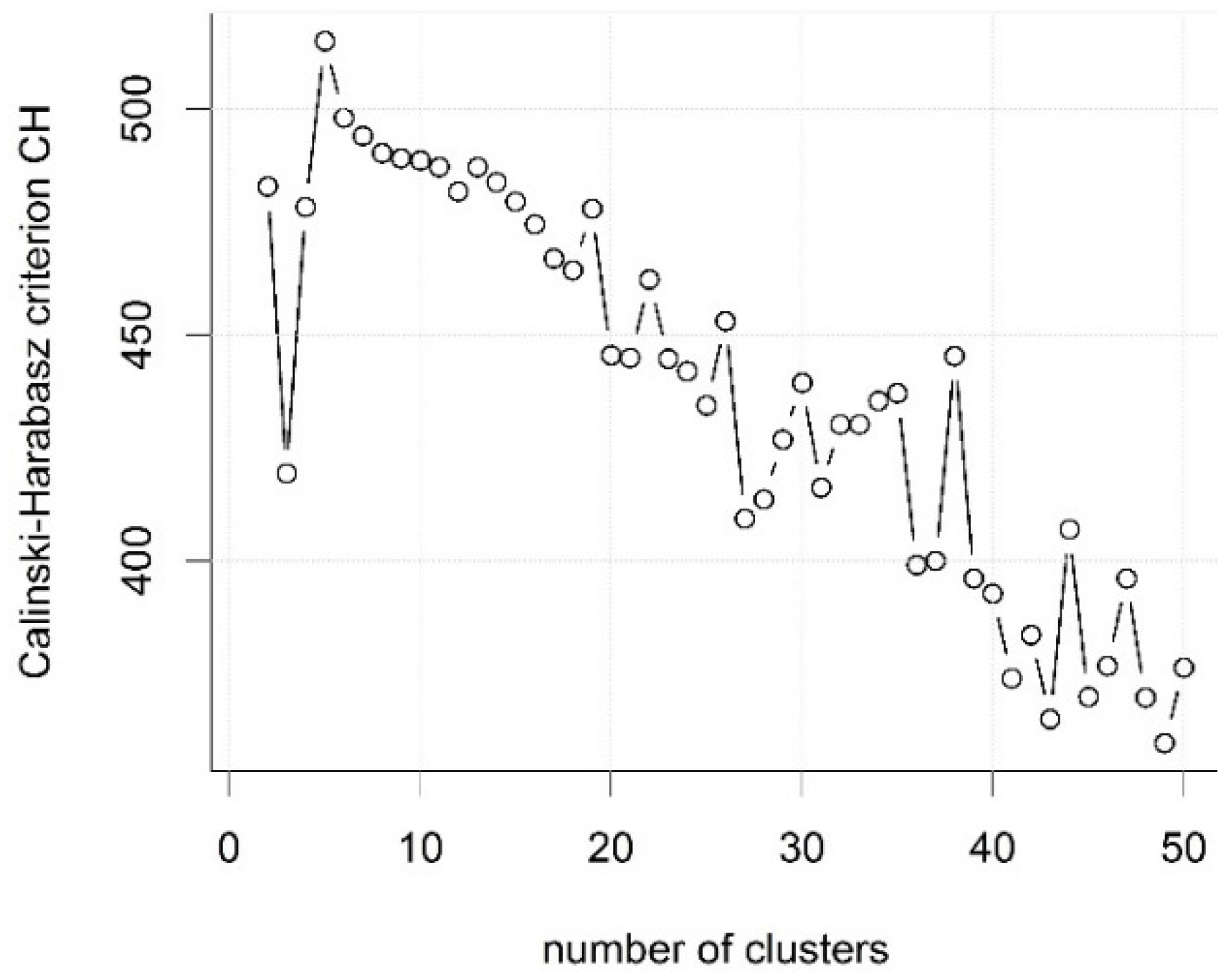
3.2. Offline Classification Using k-Means Clustering

Offline classification using k-means clustering was first performed for all rain events in the calibration dataset described in Section 2. The three principal components derived in the previous section were applied to characterize the rain events and the $CH$ criterion described in Section 2 was evaluated for different numbers of clusters $K$. The result of this analysis is shown in Figure 3. A total of $K=5$ clusters maximized the criterion and this was therefore considered the optimal number of clusters for the classification of the dataset.

To identify whether the rain events in a cluster should be considered as being of “high” or “low” variability, we used the standardized identification variables described in Section 2 and averaged them for all rain events within a cluster. The outcome of this procedure is shown in

Table 3. Standardized identification variables averaged over all rain events with each cluster and classification into events of high and low variability.

Cluster	Mavint	Sdavint	Spatsd	Maxrmax	Sdrmax	Mnlen	Mdev	Variability in Rain Event	Events in Cluster
1	6.15	6.30	4.91	4.39	4.91	1.28	3.40	High	6
2	0.63	0.47	0.78	0.87	1.00	0.40	0.72	High	51
3	−0.43	−0.42	−0.36	−0.36	−0.46	−0.94	−0.28	Low	217
4	−0.24	−0.17	−0.43	−0.40	−0.34	1.06	−0.53	Low	163
5	1.76	1.60	3.11	2.96	3.18	0.09	2.41	High	17
								SUM	454

. A feature value greater than zero implies that rain events in this cluster mostly have larger values for this feature than the average over all rain events. As all considered features characterize the variability of rain events, clusters with mean feature values larger than zero may be considered as containing rain events of “high variability” and the events were marked accordingly. Clusters 3 and 4 were considered to contain rain events of low variability as they generally yielded low values of the identification variables, while the other clusters were considered to contain rain events of high variability. A total of 68 out of 74 events classified as being of high variability took place in the summer period which we defined as starting on 1 May and ending on 31 October.

The classification derived for the calibration dataset was subsequently applied to the validation dataset by computing the standardized identification variables for the rain events in the same manner, reducing the dataset to three principal components using the loadings derived for the calibration period (Table 2) and by performing k-means classification using the cluster centres shown in Table 3. This classification of the rain events in the validation period then formed the reference for the online classification approaches.

3.3. Temporal and Spatial Variability of the Event Groups Identified

The classification obtained in the previous section is somewhat arbitrary, as the properties and thresholds characterizing event variability were freely defined. Ideally, the classification results obtained using the scheme described above, would be compared to an expert classification, but such a classification was not available for the considered dataset. However, we investigated the degree of spatial and temporal variability in the two classes by deriving covariograms and autocorrelations for the events in the two classes.

Figure 4 shows the correlograms derived for rain events classified as “high” and “low” variability, respectively. Clearly, the measurements at different gauge locations are correlated over much longer distances for events of “low” variability, while correlation coefficients become small already for short distances for events classified as being of “high” variability.

Similarly, rainfall observations demonstrate higher autocorrelations for rain events classified as “low” variability than for those classified as “high” variability (Figure 5). Thus, we considered the two classes of rain events distinctly different in terms of spatial and temporal variability.

3.4. Identifying Convective Rain Events in an Online Setting

As a final step, methods for identifying rain events of “high” and “low” variability in an online setting were investigated. We quantify speed and accuracy of identification separately. Ideally, rain events of high variability should be identified as soon as possible after the start of the rain event with high reliability, for example, to be able to switch between operational modes or forecast models. At the same time, it is important not to falsely identify events of “low” variability as having “high” variability.

Table 4. Classification results during the validation period (1078 events total) for the different approaches considered. Lag until correct identification of high variability events in time steps (median and standard deviation), % of high variability events correctly identified anywhere in the course of an event (TH), % of low variability events correctly identified for the whole duration of the event (TL), % accuracy.

Classification Result	Threshold	k-means Clustering	QDA	Random Sampling
Lag (median)	1	2	2	0
Lag (standard deviation)	3.96	7.51	6.27	0
TH % (No. of events)	100.0% (217)	96.8% (210)	99.5% (216)	31.8% (69)
TL % (No. of events)	71.3% (614)	94.3% (812)	86.2% (742)	84.2% (725)
Accuracy % ACC = (TH + TL)/(no. of events)	77.1%	94.8%	88.9%	73.7%

summarizes how soon events of “high” variability were identified after the beginning of the rain event using the different approaches. In all approaches, most events of high variability were identified within one or two time steps (10–20 min) after the beginning of the event. However, the spread of the lag times until identification varies for the different methods and the threshold method provides the fastest identification on average (Table 4).

All three identification methods reliably identified the events of “high” variability in the validation period and missed no more than 7 out of 217 events. This is clearly a much better result than what would be obtained using random sampling. The threshold method achieves similar reliability as the more complex QDA and k-means clustering techniques, because events of high variability are mainly characterized by high rainfall intensities. However, the method also leads to the largest number of events of low variability that were falsely identified as events of high variability (“false hits”) (Table 4 and Figure 6).

The k-means and QDA approaches consider additional rainfall characteristics in the classification and were thus better able to discriminate events in an online setting as well (Table 4 and Figure 6). The k-means method produced a very small number of false hits. As it is the same method used for producing the reference classification, it can effectively reproduce those identifications in an online setting as well with recursive computation of the variables used for characterising the variability of rain events. However, the method tends to require more time to identify convective events than the QDA approach.

The QDA method was specifically trained to reproduce the reference classification using recursively computed variables for identification. Nevertheless, this method produced a much bigger percentage of false hits than the k-means approach. The reason for this behaviour was that the identification variables would generally have a much larger spread for the rain events belonging to clusters of “high variability”, resulting also in a larger variance of the normal distributions used for computing the likelihood of a data point being a member of those clusters. Hence, a data point located in between a cluster of “high” and a cluster of “low” variability would more likely be assigned to the cluster of high variability, leading to a slightly higher number of correctly identified events of “high variability”, but also a much larger number of false hits than for the k-means method where a data point is assigned to the nearest cluster using the Euclidean distance measure.

The above results indicated that the consideration of additional spatial and temporal features improves the classification of rain events. The k-means method provided a reliable identification of events of “high variability” with a low number of false hits. The fastest identification of events of “high variability” was provided by the threshold method, however, at the expense of a large number of false hits. The results need to be verified against an expert classification, as the methodology so far is solely data-driven. In addition, atmospheric processes vary geographically and different classification results may be obtained in different regions.

4. Conclusions

We have demonstrated that k-means clustering can be a useful technique for objective classification of rain events in an offline setting after training the approach in a calibration period. Such an approach allows for the consideration of more characteristics of a rain event than simpler classification approaches based on, for example, a threshold on the maximal observed rain intensity. At the same time, the approach is computationally efficient and can be applied to, for example, radar images without requiring additional input data.

In an online application, we were able to reliably identify rain events of high spatial and/or temporal variability, typically within 10–20 min after the beginning of an event. More complex classification approaches based on k-means clustering and quadratic discriminant analysis were implemented recursively and reduced the number of false hits in comparison to a simple threshold method, as the spatial and temporal characteristics of the rain events are better accounted for.

Further work should focus on comparing the objective classification approach against subjective expert-classifications and on identifying the rainfall features which best allow the objective classification algorithm to reproduce expert classifications.

References

1. NOAA National Weather Service Glossary. Available online: www.weather.gov/glossary/ (accessed on 29 November 2015).
2. Dotto, C.B.S.; Allen, R.; Wong, T.; Deletic, A. Development of an integrated software tool for strategic planning and conceptual design of water sensitive cities. In Proceedings of the 9th International Conference on Urban Drainage Modelling, Belgrade, Serbia, 3–7 September 2012; Prodanovic, D., Plavsic, J., Eds.; University of Belgrade-Faculty of Civil Engineering Belgrade: Belgrade, Serbia, 2012. [Google Scholar]
3. Vieux, B.E.; Vieux, J.E. Statistical evaluation of a radar rainfall system for sewer system management. Atmos. Res. 2005, 77, 322–336. [Google Scholar] [CrossRef]
4. Kirstetter, P.-E.; Andrieu, H.; Delrieu, G.; Boudevillain, B. Identification of vertical profiles of reflectivity for correction of volumetric radar data using rainfall classification. J. Appl. Meteorol. Climatol. 2010, 49, 2167–2180. [Google Scholar] [CrossRef]
5. Jonsdottir, H.; Nielsen, H.A.; Madsen, H.; Eliasson, J.; Palsson, O.P.; Nielsen, M.K. Conditional parametric models for storm sewer runoff. Water Resour. Res. 2007, 43, 1–9. [Google Scholar] [CrossRef]
6. Löwe, R.; Thorndahl, S.; Mikkelsen, P.S.; Rasmussen, M.R.; Madsen, H. Probabilistic online runoff forecasting for urban catchments using inputs from rain gauges as well as statically and dynamically adjusted weather radar. J. Hydrol. 2014, 512, 397–407. [Google Scholar] [CrossRef]
7. Philipp, A.; Bartholy, J.; Beck, C.; Erpicum, M.; Esteban, P.; Fettweis, X.; Huth, R.; James, P.; Jourdain, S.; Kreienkamp, F.; et al. Cost733cat—A database of weather and circulation type classifications. Phys. Chem. Earth 2010, 35, 360–373. [Google Scholar] [CrossRef]
8. Huth, R.; Beck, C.; Philipp, A.; Demuzere, M.; Ustrnul, Z.; Cahynová, M.; Kyselý, J.; Tveito, O.E. Classifications of atmospheric circulation patterns. Ann. N. Y. Acad. Sci. 2008, 1146, 105–152. [Google Scholar] [CrossRef] [PubMed]
9. Feidas, H.; Giannakos, A. Classifying convective and stratiform rain using multispectral infrared Meteosat Second Generation satellite data. Theor. Appl. Climatol. 2011, 108, 613–630. [Google Scholar] [CrossRef]
10. Llasat, M.-C. An objective classification of rainfall events on the basis of their convective features: Application to rainfall intensity in the northeast of spain. Int. J. Climatol. 2001, 21, 1385–1400. [Google Scholar] [CrossRef]
11. Ricciardelli, E.; Cimini, D.; Di Paola, F.; Romano, F.; Viggiano, M. A statistical approach for rain intensity differentiation using Meteosat Second Generation-Spinning Enhanced Visible and InfraRed Imager observations. Hydrol. Earth Syst. Sci. 2014, 18, 2559–2576. [Google Scholar] [CrossRef] [Green Version]
12. Thyregod, P.; Carstensen, J.; Madsen, H.; Arnbjerg-Nielsen, K. Integer valued autoregressive models for tipping bucket rainfall measurements. Environmetrics 1999, 10, 395–411. [Google Scholar] [CrossRef]
13. Thorndahl, S.; Nielsen, J.E.; Rasmussen, M.R. Bias adjustment and advection interpolation of long-term high resolution radar rainfall series. J. Hydrol. 2014, 508, 214–226. [Google Scholar] [CrossRef]
14. Schellart, A.N.A.; Liguori, S.; Krämer, S.; Saul, A.J.; Rico-Ramirez, M.A. Comparing quantitative precipitation forecast methods for prediction of sewer flows in a small urban area. Hydrol. Sci. J. 2014, 59, 1418–1436. [Google Scholar] [CrossRef]
15. Vieux, B.E.; Bedient, P.B. Assessing urban hydrologic prediction accuracy through event reconstruction. J. Hydrol. 2004, 299, 217–236. [Google Scholar] [CrossRef]
16. Achleitner, S.; Fach, S.; Einfalt, T.; Rauch, W. Nowcasting of rainfall and of combined sewage flow in urban drainage systems. Water Sci. Technol. 2009, 59, 1145–1151. [Google Scholar] [CrossRef] [PubMed]
17. Berne, A.; Krajewski, W.F. Radar for hydrology: Unfulfilled promise or unrecognized potential? Adv. Water Resour. 2013, 51, 357–366. [Google Scholar] [CrossRef]
18. Meneses, E.J.; Löwe, R.; Brødbæk, D.; Courdent, V.; Petersen, S.O. SURFF-Operational Flood Warnings for Cities Based on Hydraulic 1D-2D Simulations and NWP. In Proceedings of the 10th International Conference on Urban Drainage Modelling (UDM), Mont-Sainte-Anne, QC, Canada, 20–23 September 2015.
19. Di Paola, F.; Casella, D.; Dietrich, S.; Mugnai, A.; Ricciardelli, E.; Romano, F.; Sanò, P. Combined MW-IR Precipitation Evolving Technique (PET) of convective rain fields. Nat. Hazards Earth Syst. Sci. 2012, 12, 3557–3570. [Google Scholar] [CrossRef]
20. Kursinski, A.L.; Mullen, S.L. Spatiotemporal variability of hourly precipitation over the Eastern Contiguous United States from Stage IV multisensor analyses. J. Hydrometeorol. 2008, 9, 3–21. [Google Scholar] [CrossRef]
21. Korsholm, U.; Petersen, C.; Sass, B.; Nielsen, N.; Jensen, D.; Olsen, B.; Gill, R.; Vedel, H. A new approach for assimilation of 2D radar precipitation in a high-resolution NWP model. Meteorol. Appl. 2015, 22, 48–59. [Google Scholar] [CrossRef]
22. Nielsen, J.E.; Jensen, N.E.; Rasmussen, M.R. Calibrating LAWR weather radar using laser disdrometers. Atmos. Res. 2013, 122, 165–173. [Google Scholar] [CrossRef]
23. Pedersen, L.; Jensen, N.E.; Madsen, H. Calibration of Local Area Weather Radar-Identifying significant factors affecting the calibration. Atmos. Res. 2010, 97, 129–143. [Google Scholar] [CrossRef]
24. Baldwin, M.E.; Kain, J.S.; Lakshmivarahan, S. Development of an automated classification procedure for rainfall systems. Mon. Weather Rev. 2005, 133, 844–862. [Google Scholar] [CrossRef]
25. Jørgensen, H.K.; Rosenørn, S.; Madsen, H.; Mikkelsen, P.S. Quality control of rain data used for urban runoff systems. Water Sci. Technol. 1998, 37, 113–120. [Google Scholar] [CrossRef]
26. Institute for Technical and Scientific Hydrology Ltd. Hystem-Extran 7.7. Institute for Technical and Scientific Hydrology Ltd.: Hanover, Germany, 2015. [Google Scholar]
27. Little, M.A.; Rodda, H.J.E.; Mcsharry, P.E. Bayesian objective classification of extreme UK daily rainfall for flood risk applications. Hydrol. Earth Syst. Sci. Discuss. 2008, 5, 3033–3060. [Google Scholar] [CrossRef]
28. Venables, W.N.; Ripley, B.D. Modern Applied Statistics with S; Springer: New York, NY, USA, 2002; Volume 4. [Google Scholar]
29. Hartigan, J.A.; Wong, M.A. Algorithm AS 136: A k-means clustering algorithm. Appl. Stat. 1979, 28, 100–108. [Google Scholar] [CrossRef]
30. Oksanen, J.; Blanchet, F.G.; Kindt, R.; Legendre, P.; Minchin, P.R.; O’Hara, R.B.; Simpson, G.L.; Solymos, P.; Stevens, M.H.H.; Wagner, H. Vegan: Community Ecology Package 2014. Available online: https://cran.r-project.org/web/packages/vegan/index.html (accessed on 12 March 2015).
31. Caliński, T.; Harabasz, J. A dendrite method for cluster analysis. Commun. Stat. 1974, 3, 1–27. [Google Scholar]
32. Pebesma, E.J. Multivariable geostatistics in S: The gstat package. Comput. Geosci. 2004, 30, 683–691. [Google Scholar] [CrossRef]
33. Madsen, H. Time Series Analysis; Chapman and Hall/CRC: Boca Raton, FL, USA, 2008. [Google Scholar]
34. Storm- and Wastewater Informatics SWI. Available online: http://www.swi.env.dtu.dk/ (accessed on 12 March 2015).
Figure 1. Rain gauges in the Copenhagen area that were used in this study.
Water 08 00087 g001
Figure 2. Cumulative % of the variance in the dataset captured by the first 8 principal components.
Water 08 00087 g002
Figure 3. Calinski-Harabasz criterion CH for k-means classification with varying numbers of clusters considered.
Water 08 00087 g003
Figure 4. Correlogram (covariogram standardized by the variance of observations) for rain events of high and low variability, depicted as correlation between observations at different locations depending on the distance between these locations.
Water 08 00087 g004
Figure 5. Autocorrelation (a) and partial autocorrelation (b) for rain events of low and high variability, depicted as median (bars), 2.5% and 97.5% quantiles (dashed lines) of the values derived for each of the 34 gauges. 1 time step corresponds to 10 min.
Water 08 00087 g005
Figure 6. Number of rain events that are falsely (a) and correctly (b) identified as having “high” variability after a lag of k time steps after event start using different classification methods.
Water 08 00087 g006