Post-Processing of Stream Flows in Switzerland with an Emphasis on Low Flows and Floods

Abstract

Post-processing has received much attention during the last couple of years within the hydrological community, and many different methods have been developed and tested, especially in the field of flood forecasting. Apart from the different meanings of the phrase “post-processing” in meteorology and hydrology, in this paper, it is regarded as a method to correct model outputs (predictions) based on meteorological (1) observed input data, (2) deterministic forecasts (single time series) and (3) ensemble forecasts (multiple time series) and to derive predictive uncertainties. So far, the majority of the research has been related to floods, how to remove bias and improve the forecast accuracy and how to minimize dispersion errors. Given that global changes are driving climatic forces, there is an urgent need to improve the quality of low-flow predictions, as well, even in regions that are normally less prone to drought. For several catchments in Switzerland, different post-processing methods were tested with respect to low stream flow and flooding conditions. The complexity of the applied procedures ranged from simple AR processes to more complex methodologies combining wavelet transformations and Quantile Regression Neural Networks (QRNN) and included the derivation of predictive uncertainties. Furthermore, various verification methods were tested in order to quantify the possible improvements that could be gained by applying these post-processing procedures based on different stream flow conditions. Preliminary results indicate that there is no single best method, but with an increase of complexity, a significant improvement of the quality of the predictions can be achieved.

1. Introduction

In general, “post-processing” refers to a process of improving model outputs regarding predefined loss functions or skill scores. Within this study, post-processing encompasses a model for correcting the errors of historical simulations and real-time forecasts, as well as the estimation of the model and forecast uncertainty. Especially in the field of hydro-meteorological Ensemble Predictions Systems (EPS), the importance of post-processing has been acknowledged in order to remove systematic bias and increase forecast skill (see for example, Brown and Seo [1], Zhao et al. [2] and Hemri et al. [3], to name a few). It is also one of the major themes of the international initiative called HEPEX (Schaake et al. [4]). In this paper, error correction and predictive uncertainty models are combined into a set of different post-processing methodologies. These methodologies were tested based on two forecasting experiments running at the Swiss Federal Institute WSLto tackle two very divergent environmental problems: floods (Addor et al. [5]) and droughts (Zappa et al. [6]).

Although it has been widely accepted that post-processing can have a significant positive impact on the quality of the model predictions, there is still a need to demonstrate its usefulness and economic implications for decision makers running operational applications. One of the objectives of this study is to check whether even models producing good results could be further improved by applying simple post-processing tools. Another goal is to evaluate post-processing tools with respect to stakeholder requirements, including civil protection agencies for flooding and water reservoir managers for low-flows and flooding.

Whereas most time series-based post-processing approaches include autoregressive parameters for incorporating memory effects (e.g., Xiong and O’Connor [7]), more physically-driven models try to analyze and reproduce the underlying processes through decomposition into sub-processes with different time horizons (e.g., fast-responding surface run-off, as opposed to long-lasting sub-surface and groundwater processes). The mathematical decomposition of time series into different levels of resolution could be interpreted as a simplified statistical description of signals analogous to physical models. This partition of the processes into high- and low-frequency components could be fulfilled efficiently by the use of Fourier analysis and Wavelet Transformations (WT). Details about decomposition methods can be found in Shumway and Stoffer [8]. The combination of the WT with autoregressive time series model approaches makes it possible to correct errors caused by different geo-physical processes and, hence, linked to different time scales, simultaneously. Similar to this decomposition approach, knowledge extraction methods based on neural networks have been proposed by Jain and Kumar [9].

In addition to the minimization of these simulation/forecast errors, the most reliable Predictive Uncertainty (PU) should also be estimated. The PU is important, because it helps to improve the quality of the result and to increase trust in the result, so that stakeholders are more willing to accept and apply the results (Todini [10]).

Other statistical approaches often applied in hydrological forecasting are neural networks (see for example, Kişi [11] and Rezaeianzadeh et al. [12]) and Quantile Regression (QR) models (e.g., Weerts et al. [13]). Recently, methods have been proposed for combining QR models with neural networks in order to capture possible estimation problems stemming from non-linearities. In this paper, various approaches combining WT and QR methods based on Neural Networks (Wave-QRNN, or simply QRNN) are applied. In Section 2, these approaches are explained and tested. The concept of PU and the related verification methods are outlined in Section 3 and Section 4. Finally, after a description of the study area and data, the forecast system and the practical model implementation in Section 5, Section 6 and Section 7, the results of this study and the discussion of its applicability in different operational forecasting systems is summarized.

2. Error Correction

In the most simple case, the correction of flow forecast systems will compare the model simulation at each prediction step with the observation realized at this time and fits an auto-regressive model with time lag 1(AR(1)) to these time series of errors. However, there is a problem extrapolating this error beyond the one step ahead prediction. A generalization of the AR models is the Vector AutoRegressive(VAR) models (for example, Gilbert [14] and Zivot and Wang [15]), which describe the evolution of more variables at the same time depending on possibly different lag times for each variable.

In the work of Bogner and Kalas [16], an error-correcting method was developed combining wavelet transformations (e.g., Beylkin and Saito [17], Chou and Wang [18]) and Vector AutoRegressive Models with eXogeneousinput (Wave-VARX). The idea was to incorporate not only the most recent information of the error in the correction model, but also information with time lags of several hours and days. This could be achieved very efficiently using wavelet transformations, resulting in time series decomposed into different scales with information about the details and smoothed (i.e., high and low frequency) components for each scale separately. The wavelet-based method for the error correction in the present study is based on a non-decimated wavelet transform, which is given by the à trous algorithm (Dutilleux [19]), and has been applied for example in Benaouda et al. [20] for forecasting purposes. The resulting vectors of decomposed stream flow observations constitute the VAR model, and the decomposed predictions (simulations and forecasts) comprise the exogenous input of the correction model. In Bogner and Pappenberger [21], the results of this method were compared to simpler ARX and VARX models, indicating some significant improvements.

In standard linear regression, the average relationship between a set of predictors and the response variable is summarized with a single slope parameter describing this relationship. Therefore, linear regression models only provide a partial view of the link between the response variable and predictors specified by the conditional-mean function and by the assumption that the standard deviations of the error terms are constant (homoscedasticity). However, in hydrology, heteroscedasticity is a common phenomena, when, for example, the difference between observed and simulated stream flow values increases with rising discharge. These kinds of problems could be solved by the use of Quantile Regression models (QR), which look at changes in the different quantiles of the response specified by the conditional-quantile function [22,23,24]. The QR model facilitates the analysis of the full conditional distributional properties of the response variable, and additionally, it has the advantage of not making any assumptions about the error distribution.

Therefore, QR is a method to estimate a set of parameters ${\beta }_{\tau }$ dependent on the quantile τ, and Koenker and Bassett Jr. [22] define the τ-th regression quantile $(0<\tau <1)$ as any solution, ${\beta }_{\tau }$, to the quantile regression minimization problem:

$$\underset{{\beta }_{\tau }\in \mathrm{I}\mathrm{R}}{min}\sum _{i=1}^n{\rho }_{\tau }\left(y_i-{\xi }_{\tau }\left(x_i,{\beta }_{\tau }\right)\right)$$

(1)

where ${\rho }_{\tau }\left(y_i-\xi \left(x_i,{\beta }_{\tau }\right)\right)$ is a function of τ and $y_i-{\xi }_{\tau }\left(x_i,{\beta }_{\tau }\right)$ and is defined as:

$${\rho }_{\tau }\left(y_i-\xi \left(x_i,{\beta }_{\tau }\right)\right)=\left\{\begin{array}{cc}\tau \left(y_i-\xi \left(x_i,{\beta }_{\tau }\right)\right)\hfill & \forall y_i\ge {\xi }_{\tau }\left(x_i,{\beta }_{\tau }\right)\hfill \\ \left(\tau -1\right)\left(y_i-\xi \left(x_i,{\beta }_{\tau }\right)\right)\hfill & \forall y_i<{\xi }_{\tau }\left(x_i,{\beta }_{\tau }\right)\hfill \end{array}\right.$$

(2)

If ${\xi }_{\tau }\left(x_i,{\widehat{\beta }}_{\tau }\right)$ is formulated as a linear function of parameters and $\{x_i:i=1,...,n\}$ denote a sequence of explanatory variables, the resulting minimization problem can be solved very efficiently by linear programming methods (Koenker [24]).

Artificial neural networks turned out to be a very popular and successful method to treat non-linearity, a common phenomena in hydro-meteorology and, hence, in QR models applied in this field. The estimation of these networks is data driven and does not require restrictive assumptions about the form of the basic model. In the case of forecasting, most often, a single hidden layer feed-forward network (Zhang et al. [25]) is applied. Therefore, it consists of a set of inputs, which are connected to a set of units in a single hidden layer, which, in turn, are connected to an output. Thus, the inputs of this network correspond to the explanatory variables, $x_i$, in a regression model and the output is the dependent variable, $y_i$. In some studies AR models and neural networks have been combined into hybrid neural networks (see for example, Jain and Kumar [26] and Abrahart et al. [27]). 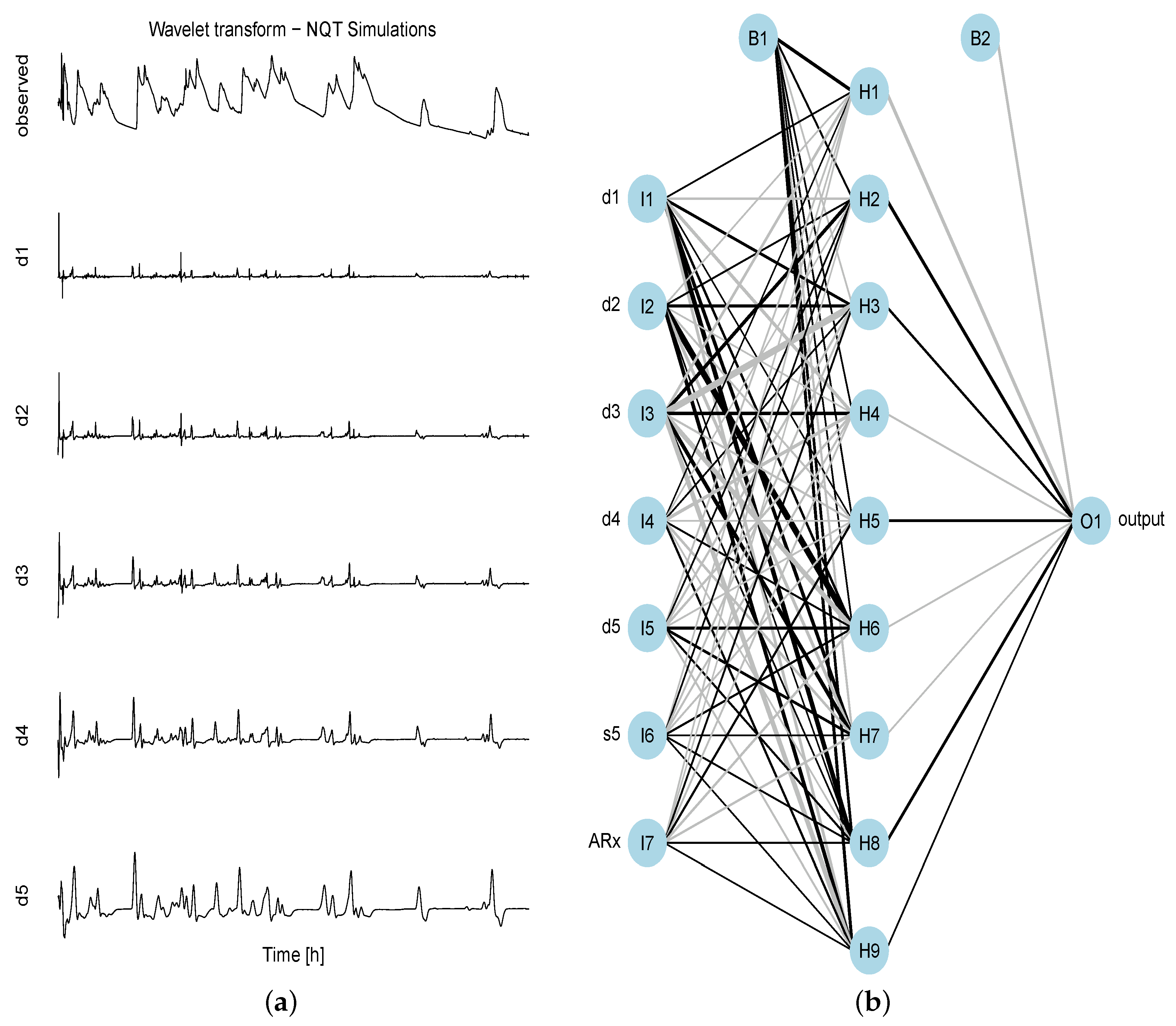White [28] presents theoretical support for the use of quantile regression within an artificial neural network for the estimation of potentially non-linear quantile models, and in Taylor [29], Cannon [30], some applications are shown. In the neural network applied in this paper, the decomposed wavelet coefficients of the simulated/forecast stream flows represent the explanatory input variables, and the observed stream flow corresponds to the output of the network (see Figure 1a,b). Although not shown in this paper, the comparison of the non-linear QRNN with the linear QR version revealed some significant improvements, especially for the first three days (≈up to hour 72). Since the accuracy and reliability of these first time intervals are very important for decision makers, the QRNN is the preferred version.

Besides the minimization of the error of the simulation and the forecast, it is essential to provide the end-users with an estimate of the uncertainty of these corrected predictions, as well. In order to make the different procedures for deriving such a predictive uncertainty comparable, all of the input and output data are transformed to the normal space beforehand applying the Normal Quantile Transformation method (NQT). In [31,32,33], the theory behind the NQT is outlined, and its application is demonstrated, e.g., in Krzysztofowicz [34] and Todini [35].

Figure 1. Wavelet decomposition and neural network. (a) Normal transformed time series of the simulated stream flow and its first five levels of wavelet decomposition (details); (b) neural network structure comprising 1 input layer: 5 nodes of details (d1,..,d5) + 1 smoothed signal decompositions (s5) of the simulation/forecast + 1 node of observed series $y_j$ for $j=1,\dots ,n-\Delta t$ (denoted as ARx) as input nodes (I1,...,I7), 1 hidden layer with 9 nodes $(H1,\dots ,H9)$ + bias coefficient B1, 1 output layer (O1), i.e., the observed series $y_i$ for $i=1,\dots ,n$ + bias coefficient B2.

Figure 1. Wavelet decomposition and neural network. (a) Normal transformed time series of the simulated stream flow and its first five levels of wavelet decomposition (details); (b) neural network structure comprising 1 input layer: 5 nodes of details (d1,..,d5) + 1 smoothed signal decompositions (s5) of the simulation/forecast + 1 node of observed series $y_j$ for $j=1,\dots ,n-\Delta t$ (denoted as ARx) as input nodes (I1,...,I7), 1 hidden layer with 9 nodes $(H1,\dots ,H9)$ + bias coefficient B1, 1 output layer (O1), i.e., the observed series $y_i$ for $i=1,\dots ,n$ + bias coefficient B2.

3. Predictive Uncertainty

Decisions related to uncertain future events need careful balancing out of the costs and the expected benefit. Therefore, decision making requires the quantification of the total uncertainty about a hydrologic predictand (such as river stage, discharge or run-off volume) in terms of a probability distribution, conditional on all available information and knowledge (Krzysztofowicz [36]). This means that in order to estimate the expected benefit, it is necessary to assess the probability density of the future occurrence as a measure of the predictive uncertainty. In Todini [35], this concept of the PU is explained, and its application in flood forecasting systems is outlined in detail in Reggiani and Weerts [37].

The Hydrological Uncertainty Processor (HUP) is applied to the ARX-based models (i.e., AR(1), VARX and Wave-VARX error corrections) for each lead time $\Delta t$ separately following the work of [36,38,39], which is based on the Bayesian formulation and a meta-Gaussian distribution family [40,41].

As already mentioned above, in the first step, all of the historical observed stream flow values and the corresponding hydrological model predictions are transformed into normal space using the quantiles associated with the order statistics (Krzysztofowicz [34] and Kelly and Krzysztofowicz [41]). Next, the a priori model will be formulated, which, in the most simple case, will rest on the assumption that the NQ transformed stream flow follows a Markovian lag one process. Furthermore, the likelihood function will rest on the assumption that the stochastic dependence between the transformed variates is governed by a simple normal-linear equation. Given that the prior density and the likelihood function are normal-linear, the theory of conjugate families of distributions (De Groot [42]) can be applied, and the posterior density can be derived.

The application of the HUP for operational flood forecasting purposes has the advantage that the fitting of the HUP to historical data can be calculated off-line, and only a small set of estimated parameters will have to be stored. The back-transformation of the corrected predictions and their probability density functions (pdfs) to the real-space is based on Generalized Additive Models (GAM; Hastie and Tibshirani [43]) in order to avoid problems possibly arising for extreme values (more details can be found in Bogner et al. [44]).

The QRNN results in direct estimates of the inverse cumulative density function (i.e., the quantile function), which in turn allows the derivation of the predictive uncertainty (see for example, [45,46,47]), where the application of the QR in order to estimate Predictive Uncertainties (PUs) is outlined. If the number of estimated quantiles within the domain $\{0<\tau <1\}$ is sufficiently large, the resulting distribution could be considered as continuous. In Quiñonero Candela et al. [48], the cdf, respectively pdf, is constructed by combining step interpolation of probability densities for specified τ-quantiles with exponential lower and upper tails. In this study, the pdf is constructed by monotone re-arranging the τ-quantiles and estimating a log-normal distribution to these quantiles for each lead-time $\Delta t$.

Another more straightforward approach could be the estimation of the parameters of the predictive distribution directly with a conditional density estimation neural network (Cannon [30] and Li et al. [49]). However, this direct method yielded discontinuities across forecast horizons with rather unrealistic jumps between consecutive lead times, which degrades the applicability of this method.

The advantage of the proposed quantile re-arranging and the estimation of the log-normal distribution is two-fold and prevents efficiently known problems occurring with QR: firstly, it eliminates the problem of the crossing of different quantiles (i.e., the unrealistic, but possible outcome of the non-linear optimization problem yielding lower quantiles for higher stream flow values (Chernozhukov et al. [50]); e.g., the value of the 0.90 quantile is higher than the value of the 0.95 quantile), and secondly, it permits the extrapolation to extremes not included in the training sample (Bowden et al. [51]).

In order to demonstrate the improvement achieved by the proposed method combining wavelets and QRNN for extreme stream flow conditions, i.e., low-flow and flooding, different verification measures will be applied and tested.

4. Verification

The objective of this study will not be the development of novel verification tools, but the usage of already existing ones and combining hydrological and meteorological evaluation criteria. Different verification measures are applied depending on whether the performance of deterministic time series or probabilistic densities should be evaluated.

4.1. Deterministic Evaluation

The quality of point prediction models, such as the deterministic output of a hydrological model, will be usually assessed with the well-known Mean Absolute Error (MAE) and the Nash–Sutcliffe (N-S) coefficient [52]. In order to estimate the percentage of improvements of the correction method in comparison to the uncorrected simulation/forecast, the failure index, which was proposed recently by Madadgar et al. [53], will be applied.

Basically, the idea of this failure index is to look at the movement of the correction and to count how often the simulated/forecasted value gets closer to the observed value applying a correction method. Thus, two different kinds of failures could result from the correction/movement: Failure 1 corresponding to a movement in the opposite direction away from the observation; Failure 2 results from a movement in the right direction, but more than two times the distance δ between the uncorrected simulated and the observed value (see Figure 2).

Figure 2. Example of the measure of the failure index (i.e., failure ratio).

Figure 2. Example of the measure of the failure index (i.e., failure ratio).

Larger values of the failure ratio mean that the correction method has more frequently affected the performance negatively, and thus, the efficient performance of the correction method manifests in a small failure index.

4.2. Probabilistic Evaluation

In Gneiting et al. [54] and Gneiting and Balabdaoui [55], the term calibration is used for describing the statistical consistency between the distributional forecasts and the observations and is a joint property of the predictions and the events that materialize. An analysis tool for assessing the calibration of ensemble forecasts is the verification rank or Talagrand histogram (e.g., Jolliffe and Stephenson [56]), and analogously for pdf forecasts, the Probability Integral Transform (PIT) was proposed by Dawid [57]. Quite often in the hydro-meteorological literature, the term reliability is used instead of calibration; thus, forecasts are called reliable if their probabilities match the observed frequencies. The predictive Quantile-Quantile (Q-Q) plot is a good way for analyzing reliability, since it is easy to interpret, and it shows how well the observations correspond to realizations from the predictive distribution (Laio and Tamea [58], Renard et al. [59]). If $F_i$ is the cdf of the random variable $Y_i$ and $y_i$ is the time series of realizations, i.e., the observed stream flow, the probability values p of $F_i\left(y_i\right)=p(Y_i\le y_i)$ will follow a uniform distribution on the interval $[0,1]$, only if the realizations $y_i$ are consistent with $F_i$.

The sharpness refers to the resolution of a probabilistic forecast and is a property of the forecast only describing the spread of the forecast pdf, i.e., the more concentrated the forecast pdf, the sharper the forecast. The sharpness can be evaluated visually by box-plots illustrating the width of the prediction intervals (Gneiting and Balabdaoui [55]) or by some simplified indexes defined, for example, as the relative precision of the prediction (Renard et al. [59]).

4.2.1. Continuous Ranked Probability Score

The Continuous Ranked Probability Score (CRPS) addresses both the sharpness and the reliability, is defined as the integral of the Brier score at all possible threshold values t for the continuous predictand (Hersbach [60]) and can be interpreted as a general version of the mean absolute error (Gneiting and Raftery [61]). It compares the forecast probability distribution with the observation, and both are represented as cdfs. Therefore, an ensemble of predictions can be converted into a piecewise constant cdf with jumps at the different ensemble members, and the observation is a Heaviside distribution with a single step from zero to one at the observed value of the variable. In the case of QR models, the cdf is derived with quantile estimates. If F is the predictive cdf and y is the verifying observation, the CRPS is defined as:

$$\begin{array}{c}\hfill \begin{array}{c}\hfill CRPS(F,y)={\int }_{-\infty }^{\infty }{\left[F\left(t\right)-H(t-y)\right]}^{2}dt\end{array}\end{array}$$

(3)

where $H(t-y)$ denotes the Heaviside function. This measure will be used for the analysis of forecasts based on the Consortium for Small-scale Modeling-Limited-area Ensemble Prediction System (COSMO-LEPS) forecast system (Montani et al. [62]) and for the analysis of the predictive densities derived with ARX-based models and QRNN models.

4.2.2. Quantile Score

Since the output of the QRNN model will be quantiles, it seems reasonable to evaluate the performance with a skill score, which has been developed for predictive quantiles (Koenker and Machado [63] and Friederichs and Hense [64]), the so-called Quantile Score (QS). It is defined by the check function ${\rho }_{\tau }$ given in Equation (2) and sums over a weighted absolute error between quantile forecasts and observations. In Bentzien and Friederichs [65], a decomposition of the QS has been proposed, which provides information about reliability and sharpness (resolution). Thus, the information of the QS is similar to the CRPS, but whereas the CRPS averages over the complete range of forecast thresholds and probability levels, the QR looks at specific τ-quantiles; hence, it is more efficient in revealing deficiencies of different parts of the distributions, especially with respect to the tails of the distribution. However, for the verification of very low and high quantiles, a large sample size is necessary in order to estimate the score at these quantiles properly.

5. Data

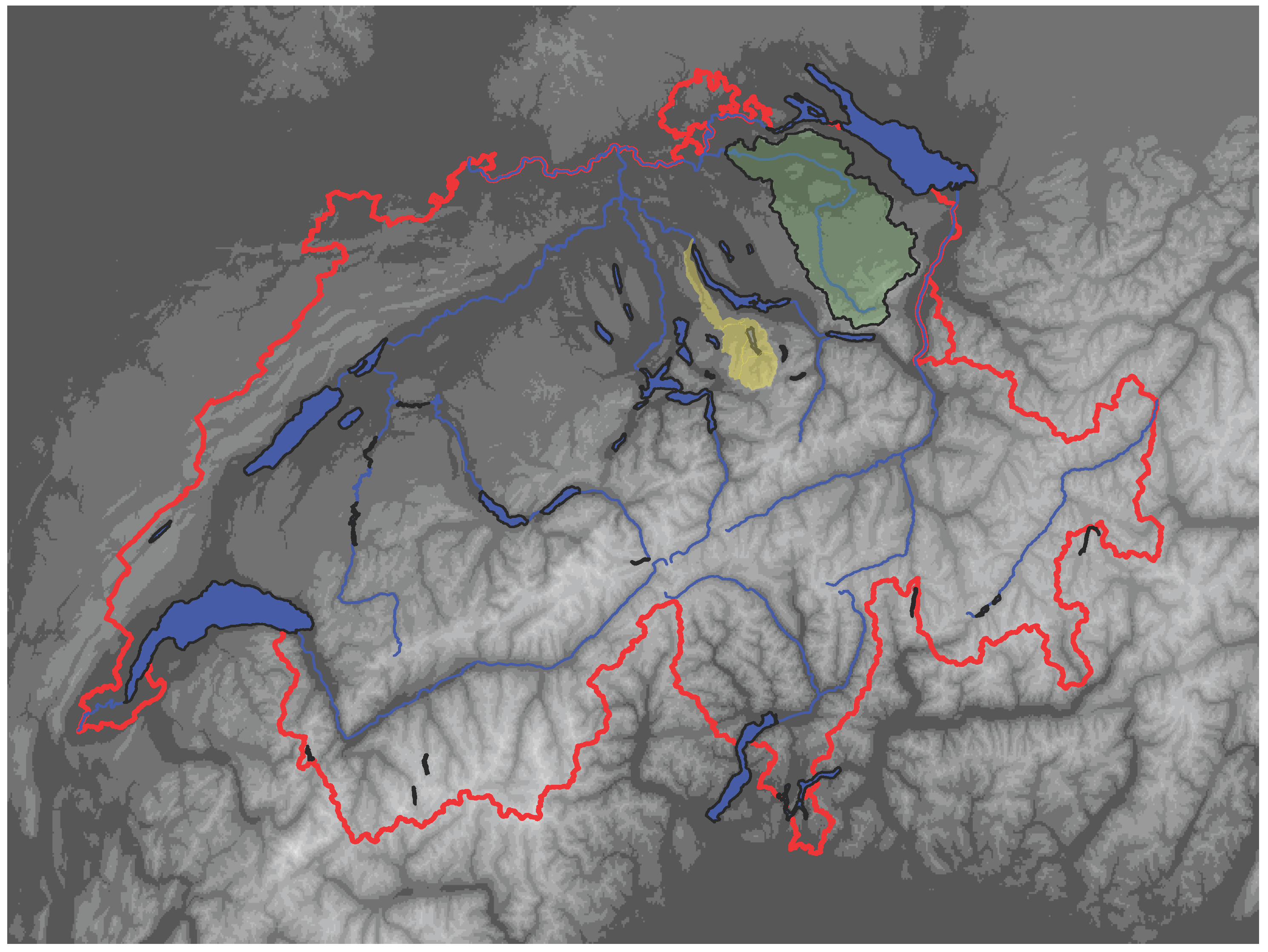
At the Swiss Federal Institute WSL, there are two forecast systems running operationally targeting two divergent objectives, one for providing information about droughts in general and low-flow conditions at selected catchments in Switzerland (Zappa et al. [6]) and one for forecasting flood events in order to protect the city of Zurich (Addor et al. [5] and Zappa et al. [66]). In Figure 3, the catchment of the Sihl, which represents the flood forecast system of Zurich, as well as the catchment of the Thur, which is taken as an example of the low-flow forecast system, are highlighted. In Table 1, some hydrological relevant characteristics of these two catchments are summarized.

The Sihl River flows through Zurich and represents the largest flood threat for this most populated city of Switzerland. To anticipate extreme discharge events and to provide decision support in case of flood risk, the hydrometeorological ensemble prediction system (HEPS) was launched operationally in 2008. The resulting hydrological forecasts are eventually communicated to the stakeholders involved in the Sihl discharge management (Addor et al. [5], Ronco et al. [67]).

The drought.ch platform provides information about ongoing and forecast droughts and water deficiencies in Switzerland. The general situation is estimated taking into account current runoff in Swiss rivers, precipitation over the last few weeks, soil moisture simulations, groundwater level, snow cover information, drought in forests, levels of lakes and reservoir lakes and the water temperature of Swiss rivers (Zappa et al. [6]). The platform does not provide official warnings, but is thought of as an information platform for a broad user group (about 500 registered users as of December 2015). The evaluated forecasts concerning the drought.ch application relate to the Thur River (Fundel et al. [68] and Joerg-Hess et al. [69]) and have been running since 2011, and the archived forecast outcomes are first evaluated here.

Figure 3. Catchment of the Sihl (yellow) and the Thur (green), which represent the flood forecast, respectively the low flow forecast system. Swiss GIS elements reproduced with the authorization of swisstopo (JA100118).

Figure 3. Catchment of the Sihl (yellow) and the Thur (green), which represent the flood forecast, respectively the low flow forecast system. Swiss GIS elements reproduced with the authorization of swisstopo (JA100118).

Table 1. Some characteristic values of the 2 catchments. MHQis the mean annual maximum daily discharge. NM${}_7$Qis obtained by taking the moving averages of the daily observations with a window size of 7 days for each year and then estimating the mean of the annual minima of these averaged series.

Catchment	Surface Area km2	Mean Elevation m.a.s.l.	MHQ m3/s	NM7Q m3/s
Sihl	336	1060	132	2.8
Thur	1696	770	592	9.2

Table 1. Some characteristic values of the 2 catchments. MHQis the mean annual maximum daily discharge. NM${}_7$Qis obtained by taking the moving averages of the daily observations with a window size of 7 days for each year and then estimating the mean of the annual minima of these averaged series.

Catchment	Surface Area km2	Mean Elevation m.a.s.l.	MHQ m3/s	NM7Q m3/s
Sihl	336	1060	132	2.8
Thur	1696	770	592	9.2

6. Forecast Systems

The stream flow forecasts of the Sihl and the Thur catchment are driven by the COSMO-Limited-area Ensemble Prediction System (LEPS, Montani et al. [62]), which is nested into the ensemble prediction system of ECMWF(Molteni et al. [70], Buizza et al. [71]). COSMO stands for the Consortium for Small-scale Modeling. The Sihl flood forecasting system is supplemented operationally with two deterministic numerical weather predictions versions of the COSMO produced at MeteoSwiss, the COSMO-2 and COSMO-7 (see Table 2); however, this paper will focus on the application and verification of COSMO-LEPS alone.

These limited-area atmospheric forecasts are taken as input for the hydrological model. The stream flows are estimated by the use of the conceptual hydrological model PREVAH (Precipitation-Runoff-EVApotranspirationHRU Model). Originally, PREVAH was based on hydrologic response units (HRU), i.e., clusters of raster grids of similar hydrological properties (Gurtz et al. [72]). This HRU version is used for the Sihl catchment. Because of the elongated shape of the basin, proper flood wave propagation is essential. Therefore, PREVAH is coupled with a hydraulic model called FLORIS, a commercial 1D simulation program developed in the 1990s by the Laboratory of Hydraulics, Hydrology and Glaciology (VAW) of the ETHZurich. Recently, a fully-distributed PREVAH version was developed, which is targeted for low-flow and water resources assessment studies (Kobierska et al. [73]), and it is used within the drought.ch platform, hence at the Thur catchment, as well (e.g., Joerg-Hess et al. [69] and Speich et al. [74]). Further information about PREVAH’s structure, physics, tunable parameters and tools can be found in Viviroli et al. [75].

Table 2. Numerical weather prediction systems. COSMO-LEPS, Consortium for Small-scale Modeling-Limited-area Ensemble Prediction System.

System	Spatial Resolution km2	Forecast Horizon h	Ensemble Members	Update Cycle h
COSMO-2	2.2 × 2.2	24	-	3
COSMO-7	6.6 × 6.6	72	-	8
COSMO-LEPS	7 × 7	132	16	24

Table 2. Numerical weather prediction systems. COSMO-LEPS, Consortium for Small-scale Modeling-Limited-area Ensemble Prediction System.

System	Spatial Resolution km2	Forecast Horizon h	Ensemble Members	Update Cycle h
COSMO-2	2.2 × 2.2	24	-	3
COSMO-7	6.6 × 6.6	72	-	8
COSMO-LEPS	7 × 7	132	16	24

7. Modeling Implementation

For the calibration of the ARX and the QRNN parameters, historical time series of observations and corresponding model simulations are necessary. Since hydro-meteorological forecasts show a strong lead time dependence, it is necessary to estimate these model error parameters for each lead time separately in order to combine these estimates with real-time forecasts. For both catchments, the series are decomposed into six levels of detail. The waveVARX and VARX models include three time lags each, whereas the ARX is a simple AR(1) model.

The QRNN setting is a single hidden layer feed-forward network, where the input layer comprises eight nodes (six nodes for the details, one node of the smoothed wavelet coefficients and one node for the time lagged observed series $y_j$ up to the last available time step $j=1,...,n-\Delta t$); the hidden layer consists of 10 nodes plus the bias coefficient and one output layer plus the bias coefficient (see Figure 1b for an example with seven input nodes). The number of hidden layer nodes has been chosen by trying to balance the computational costs and capturing as much as possible the non-linear complexity of the data. The number of quantiles τ was set to nine: $\tau =\{0.01,0.05,0.1,0.25,0.5,0.7,0.9,0.95,0.99\}$.

In order to avoid the well-known problems of crossing quantiles and the extrapolation of neural networks, the quantiles of the QRNN method have been approximated for each lead time by a log-normal distribution. Other possibilities have been tested, as well, like the combination of a monotone rearrangement method [50] with the method proposed by [48] of the step interpolation of the quantiles and exponential tails. The step-interpolation method would be advantageous in the case of multi-modal distributions or distributions departing from the lognormal assumption, which is, however, not the case in the analyzed datasets. Thus, the second approach is preferred, because the step-interpolation has more computational time consumption and showed no improvements at all.

Additionally, two different ways of density aggregations have been tested for deriving the density of the total ensemble. One method is based on averaging the quantiles of the 16 ensemble members directly, and the other one is calculated by averaging the probabilities derived from the approximated pdfs similar to the work of [76], which will be called QRNN-q-ave., respectively QRNN-p-ave.

For the ARX-based models, the PU is estimated for each lead time by assuming that the pdf of the 16 ensemble members could be approximated with a normal distribution, as they were all, as previously mentioned, transformed in the normal space. Thus, the uncertainty stemming from the model and the uncertainty from the forecast can be integrated into the total PU as outlined in the work of [38]. A detailed report about these methodologies of ensemble aggregation is under preparation.

8. Results

The calibration and evaluation of the applied post-processing methodologies is separated into two parts: the first part is based on historical observations and corresponding simulations, which are split into two parts, one half for calibrating and one half for validating the error correction models. This second half of the first part is used for calibrating the HUP parameters, as well as for the ARX-based models. The second part is used for running the model in quasi-operational mode applying the fitted correction and uncertainty parameters to the members of the ensemble forecasts and for validating the forecasts. In Table 3, the different periods available for the two catchments are summarized.

Table 3. Time ranges and periods available for the calibration and evaluation of the Thur and the Sihl catchments. HUP, Hydrological Uncertainty Processor.

Catchment	Time Resolution	Observation/Simulation		Forecasts
		Calibration	Validation/Calibration (HUP)	Validation
Thur	daily	1981–1995	1996–2010	2011–2015
Sihl	hourly	2009–2011	2011–2014	2011–2015

Table 3. Time ranges and periods available for the calibration and evaluation of the Thur and the Sihl catchments. HUP, Hydrological Uncertainty Processor.

Catchment	Time Resolution	Observation/Simulation		Forecasts
		Calibration	Validation/Calibration (HUP)	Validation
Thur	daily	1981–1995	1996–2010	2011–2015
Sihl	hourly	2009–2011	2011–2014	2011–2015

8.1. Thur Catchment

For the Thur catchment, a period of 30 years (1981–2010) of historical daily observations and simulations was available, and the first 15 years were used for calibrating the ARX-based and the QRNN parameters. The second half of this period was used for validation and for calibrating the HUP parameters necessary for the ARX-based models. The forecast horizon of the COSMO-LEPS forecasts is 5.5 days, and therefore, a set of five different parameters need to be estimated (the first half day is disregarded because of the time delay between forecast initialization and availability).

These parameters are applied to the archived forecast data from 2011–2015, and the verification measures were calculated. Each of the 16 ensemble members of the COSMO-LEPS-based forecast is treated as a single deterministic forecast and corrected individually. The deterministic verification measures are then calculated by averaging the 16 members. In the case of the QRNN, where the result was comprised of a set of different quantile estimates ranging from 0.01–0.99 for each ensemble member, only the median is used and averaged for further evaluation.

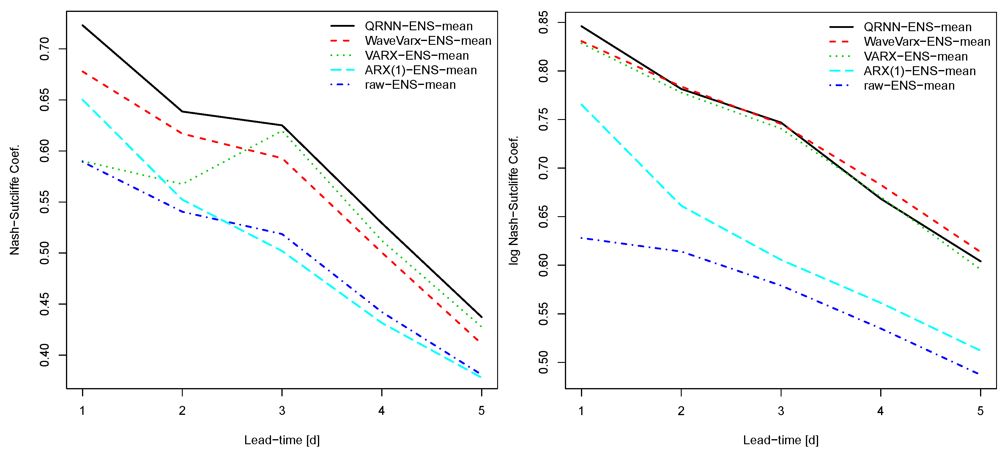
The results are evaluated applying the classical N-S coefficient for flood forecast, the logarithmic N-S for low-flow verification and the failure ratio. The CRPS and the quantile score are used for evaluating the behavior of the ensemble forecast system (see Figure 4, Figure 5, Figure 6 and Figure 7).

Figure 4. Classical Nash–Sutcliffe (N-S) coefficients (left) and logarithmic N-S (right) for different post-processing methods applied to forecasts based on COSMO-LEPS and for the period 2011–2015 for the Thur catchment.

Figure 4. Classical Nash–Sutcliffe (N-S) coefficients (left) and logarithmic N-S (right) for different post-processing methods applied to forecasts based on COSMO-LEPS and for the period 2011–2015 for the Thur catchment.

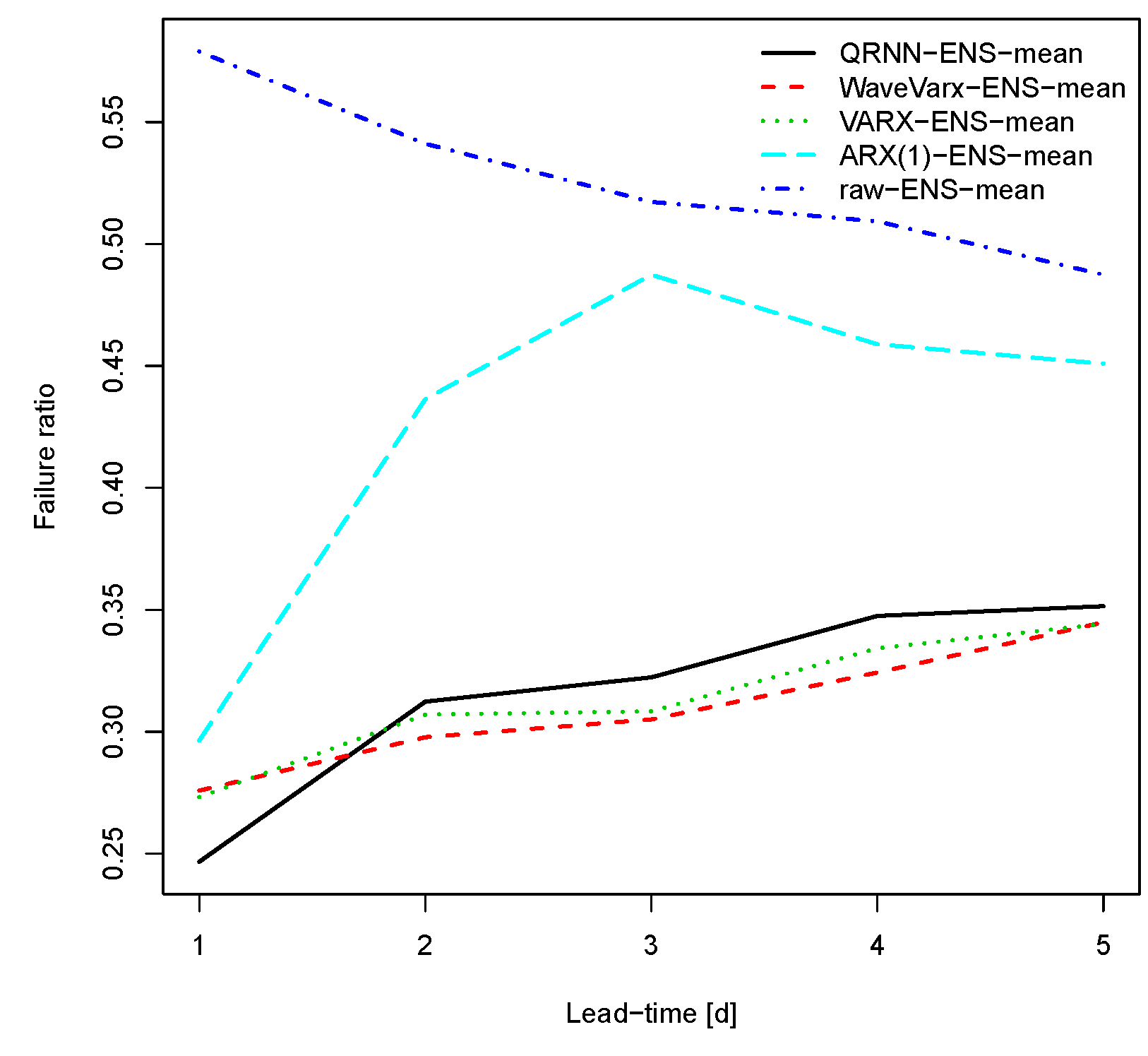
Figure 5. Failure ratio for different post-processing methods for the Thur catchment. A failure ratio below 0.5 means that the (post-processed) forecast is better than the reference model simulation.

Figure 5. Failure ratio for different post-processing methods for the Thur catchment. A failure ratio below 0.5 means that the (post-processed) forecast is better than the reference model simulation.

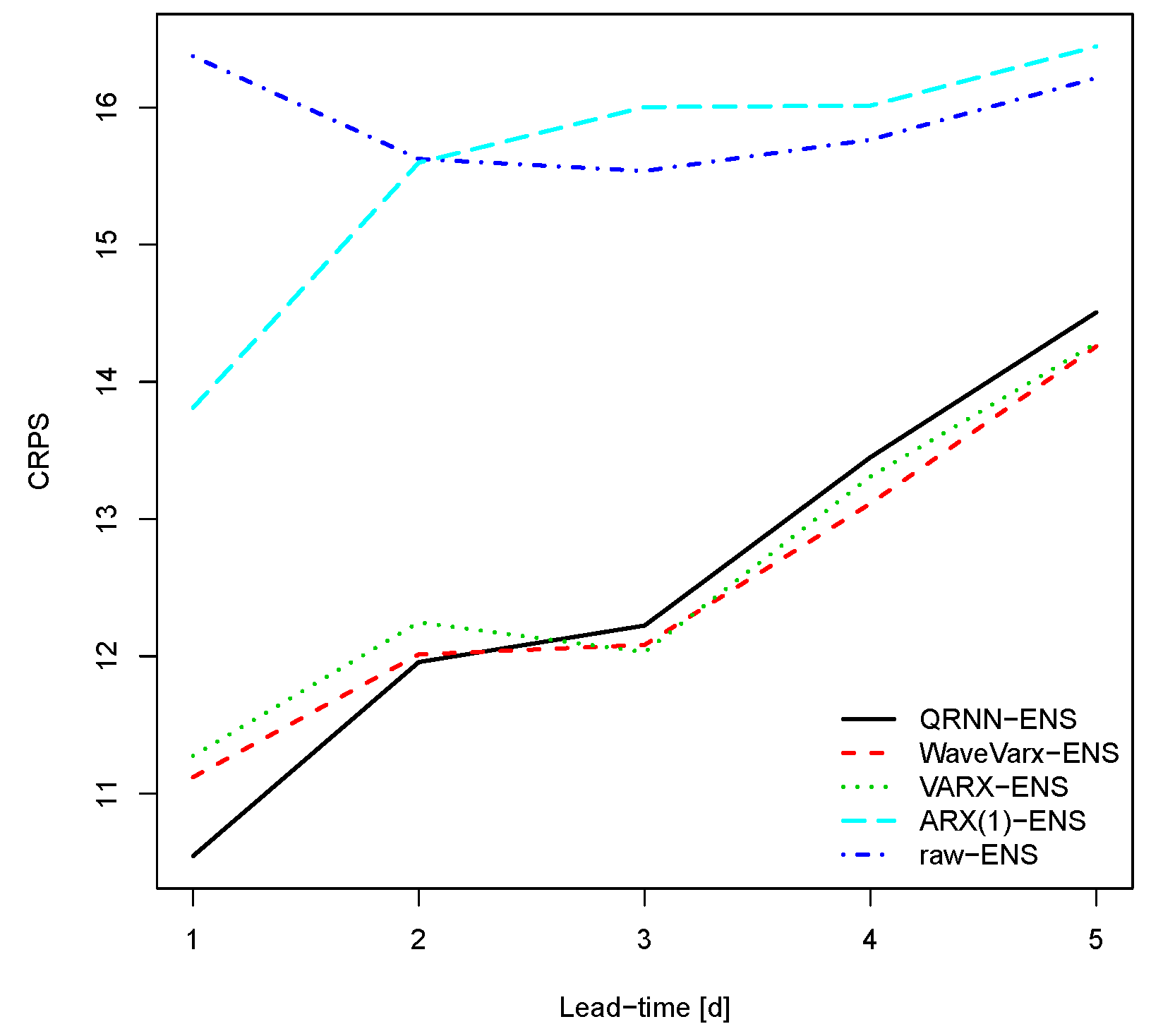
Figure 6. Continuous Ranked Probability Score (CRPS) for the Thur catchment. The CRPS is negatively oriented, which means the lower the better.

Figure 6. Continuous Ranked Probability Score (CRPS) for the Thur catchment. The CRPS is negatively oriented, which means the lower the better.

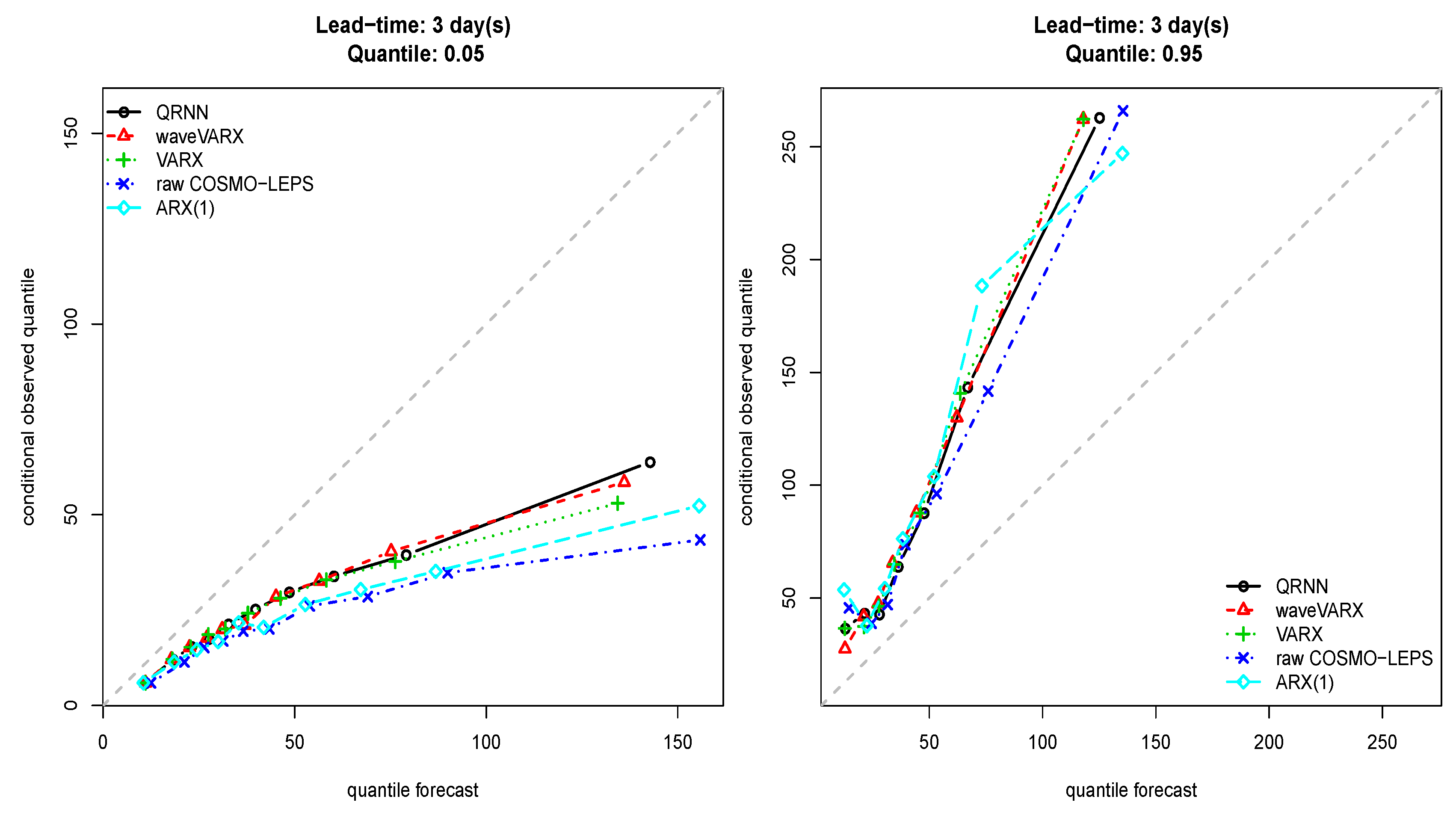
Figure 7. Quantile score for the 0.05 (left) and 0.95 (right) quantile at a lead time of three days (Thur catchment).

Figure 7. Quantile score for the 0.05 (left) and 0.95 (right) quantile at a lead time of three days (Thur catchment).

8.2. Sihl, Zurich

Since the operational forecast for the Sihl is running hourly, a set of 132 parameters for the ARX-based and QRNN models needs to be estimated, i.e., for each hour of the forecast horizon of the COSMO-LEPS.

Another difference between the Sihl and the Thur catchment is in the way the single ensemble members are incorporated in the post-processing model.

In the case of the Sihl catchment, the lognormal approximation of the quantiles (wave-QRNN-logN) method and the two different density aggregation methods, the quantile, respectively, the probability averaging method (QRNN-q-aver and QRNN-p-aver; see Section 7), were applied in order to take advantage of as much information as possible from the ensembles.

To calibrate the post-processing models at the Sihl, a period from 2009–2014 was available, where the first half was used for estimating the ARX-based model and QRNN parameters and the second half was used for validation and to calibrate the HUP parameters (Table 3, Figure 8). To verify the operational forecast system (i.e., the hindcast) itself, a period from 2011–2015 was analyzed (Figure 9). Besides the CRPS, an example of a reliability verification, the predictive quantile-quantile plot, is shown. In this graph, the $z_i$, the probability integral transformed variables, are plotted versus their empirical cumulative distribution function, $R_i/n$ (where $R_i$ are the ranks of the ordered vector of $z_i$’s, $i=1,\dots ,n$).

The model has been running quasi-operational with the COSMO-LEPS forecasts (hindcast) for approximately five years (2011–2015). There is a temporal overlap of the model validation and the hindcast period of four years (2011–2014); however, the meteorological datasets are different (observed data for the validation period, respectively COSMO-LEPS forecast data during the hindcast period); thus, the resulting stream flow series show differences, as well. The forecast time resolution is hourly; however, the forecasts are updated only once per day, when the new 12:00 o’clock run of the COSMO-LEPS forecast becomes available.

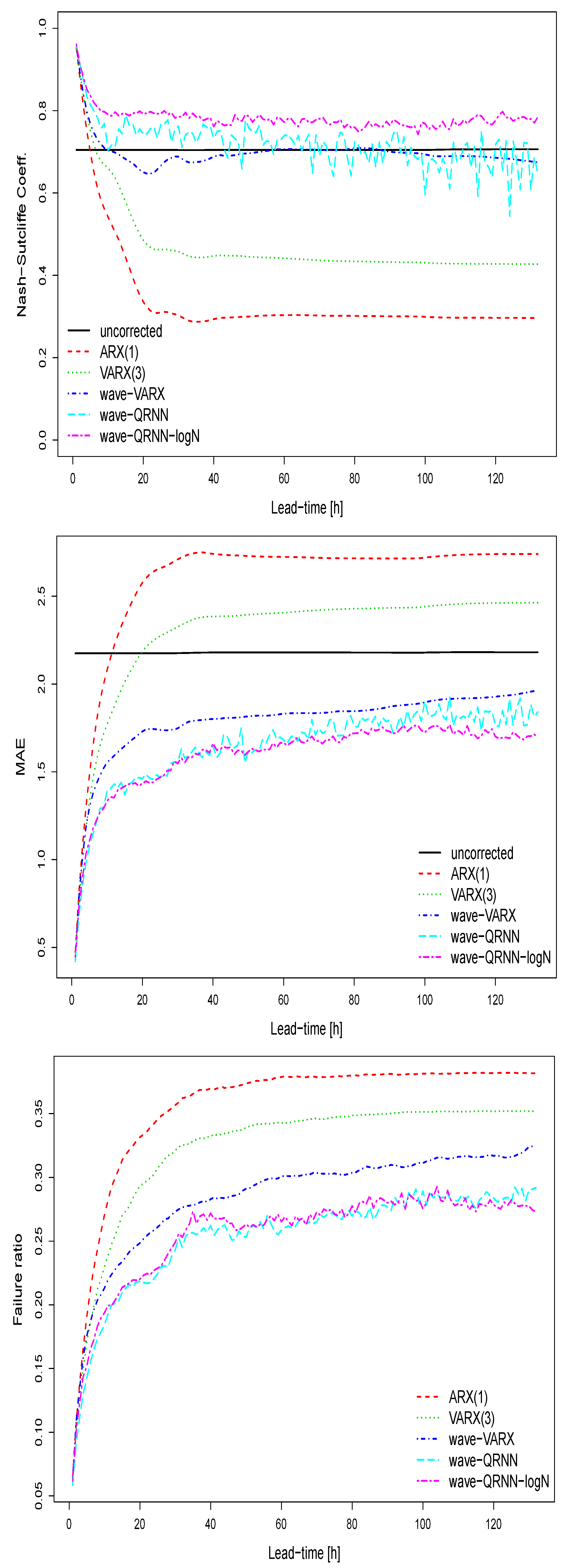
Figure 8. Deterministic verification measures for the uncorrected and post-processed model simulations for the validation period 2012–2014 at the Sihl (Zurich). Upon: the Nash-Sutcliffe efficiency coefficient; Middle: the mean absolute error; Bottom: the failure ratio.

Figure 8. Deterministic verification measures for the uncorrected and post-processed model simulations for the validation period 2012–2014 at the Sihl (Zurich). Upon: the Nash-Sutcliffe efficiency coefficient; Middle: the mean absolute error; Bottom: the failure ratio.

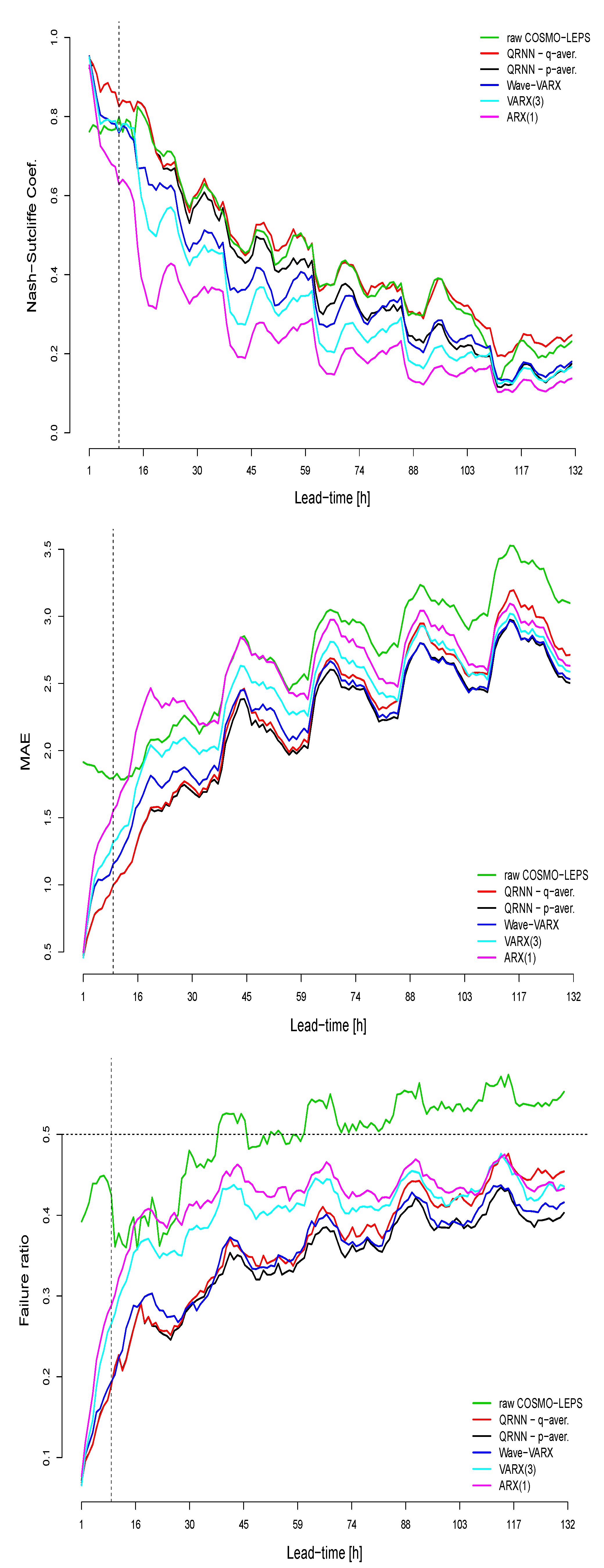
Figure 9. Deterministic verification measures for the uncorrected and post-processed forecasts (i.e., hindcasts) for the verification period 2011–2015 at the Sihl (Zurich). Upon: the Nash-Sutcliffe efficiency coefficient; Middle: the mean absolute error; Bottom: the failure ratio. The dashed vertical line in black indicates the time, when the hydrological forecast starts to be driven by the meteorological forecast, which is delayed a couple of hours because of technical restrictions.

Figure 9. Deterministic verification measures for the uncorrected and post-processed forecasts (i.e., hindcasts) for the verification period 2011–2015 at the Sihl (Zurich). Upon: the Nash-Sutcliffe efficiency coefficient; Middle: the mean absolute error; Bottom: the failure ratio. The dashed vertical line in black indicates the time, when the hydrological forecast starts to be driven by the meteorological forecast, which is delayed a couple of hours because of technical restrictions.

Figure 10. Probabilistic verification measures for the uncorrected and post-processed forecasts (i.e., hindcasts) for the verification period 2011–2015 at the Sihl (Zurich). Upon: Continuous ranked probability score; Bottom: example of a predictive Quantile-Quantile (Q-Q) plot for a lead-time of 72 h. In the Q-Q plot, $z_i$, the probability integral transformed variables, are plotted versus their empirical cumulative distribution function, $R_i/n$ (where $R_i$ are the ranks of the ordered vector of $z_i$’s, $i=1,\dots ,n$).

Figure 10. Probabilistic verification measures for the uncorrected and post-processed forecasts (i.e., hindcasts) for the verification period 2011–2015 at the Sihl (Zurich). Upon: Continuous ranked probability score; Bottom: example of a predictive Quantile-Quantile (Q-Q) plot for a lead-time of 72 h. In the Q-Q plot, $z_i$, the probability integral transformed variables, are plotted versus their empirical cumulative distribution function, $R_i/n$ (where $R_i$ are the ranks of the ordered vector of $z_i$’s, $i=1,\dots ,n$).

9. Discussion

9.1. The Thur Catchment

It is interesting to see that both Nash–Sutcliffe efficiency measures for the mean COSMO-LEPS clearly indicate that the post-processing significantly improves the system for all lead times in comparison to the uncorrected raw ensemble mean (Figure 4) for the Thur catchment. However, the logarithmic N-S for evaluating low-flow conditions shows, apart from the most simple AR(1) model, very similar improvements across all methods, whereas there are differences looking at the classical N-S, which is known to be more sensitive to flood events. The failure ratio also shows similar results (Figure 5), indicating that the more complex post-processing methods produce similar improvements in the quality of the forecast for the Thur catchment. Regarding the probabilistic behavior of the forecast, the CRPS produced similar results to the failure ratio (Figure 6), which is confirmed when looking at the quantile score for low-flow conditions. In Figure 7, the quantile scores for probability levels of 0.05 and 0.95 and for lead times of three days are shown. In this example, the wave-VARX and the QRNN methodology are superior for low-flows (0.05 level), being closer to the 1:1 line. However, in general, all forecasts overestimate the very low observed quantiles, whereas the opposite happens for high quantiles (shown on the left in Figure 7).

9.2. Sihl, Zurich

The results of the Sihl catchment for the model validation period (2011–2014) clearly indicate the improvement due to applying the different post-processing methods, with the QRNN method (see Figure 8) being the best. In all three measures (MAE, Nash–Sutcliffe coefficient and failure ratio), the QRNN method with quantiles approximated by a log-normal distribution (wave-QRNN-logN) obtained the best results. For the validation period, the meteorological observations are used as input; hence, the MAE and the Nash–Sutcliffe coefficients remained constant for the uncorrected predictions for all lead times. The results of the hindcast period (2011–2015) driven by meteorological forecasts are similar to the validation period for the deterministic verification measures based on model averages and the CRPS, as well (Figure 9 and Figure 10). Although these first results show no clear preference regarding the averaging method applied to the QRNN method, quantile averaging (QRNN-q-ave.) or probability averaging (QRNN-q-ave.), in daily operational usage, the QRNN-quantile-averaging method results more often appeared under-dispersive and produced rather unreliable and overconfident ensembles forecasts.

Because of the limited period for verification, only a few flood events were observed during the hindcast period. As mentioned previously, the hourly forecasts of the next 5.5 days (i.e., 132 h) are issued once per day (after the 12:00 COSMO-LEPS forecast run has been completed). If the forecast peak is persistent, it will appear the first time in the forecast with a lead time of five days and subsequently at a lead time of four till one. Usually, the biggest differences between observations and simulation/forecast will occur at these times of the peaks, and therefore, the verification measure will show the biggest changes at these times. Consequently, the measures are shifted from a lead time of 1–5. Thus, these single peaks dominate the scores, which explains the strong periodic daily cycle occurring in Figure 9 and Figure 10. Unfortunately, this limited amount of flood events prevents a meaningful application of the quantile score for extreme probability levels. In place of the QS, the predictive Q-Q plot is shown for a lead time of 72 h, although the same is valid for the other lead times, as well. It is interesting to see that the raw forecast is much more unreliable in comparison to the post-processed forecast, showing problems with the spread of the ensemble forecast (i.e., it is under-predictive in the example). This lack of reliability is important to point out, because, for example, the Nash–Sutcliffe efficiency of the raw forecast and the QRNN method are very similar for all of the lead times. These results highlight once again the importance of looking at different verification measures.

10. Conclusions

In this paper, different post-processing methods are tested for two different applications: low-flow forecasting and flood forecasting. The tests were carried out in Switzerland using the Thur catchment for low-flow applications and the Sihl catchment for flood forecasting. Method validation was separated into deterministic (MAE, Nash–Sutcliffe coefficient and the recently-developed failure ratio) and probabilistic evaluation measures (CRPS, predictive quantile quantile plot). In order to test the forecast quality regarding low-flow conditions, the logarithmic Nash–Sutcliffe measure and the novel quantile score were evaluated for the Thur catchment, which is is also part of the drought.ch information platform. For the evaluation of the flood warning system at the Sihl/Zurich, the same measures have been applied, but not the logarithmic Nash–Sutcliffe and quantile score, because of the limited forecast period available for analyzing.

In general, all of the results confirmed the positive impact of post-processing for both experiments, even though the raw model simulations showed very good results. Only for the most simple ARX(1) model, the improvements were not significant within a few time steps ahead and should not be used for low-flows or for flood event forecasts. The new method of quantile regression neural network produced some additional improvements, but further tests and longer forecast series are needed for a thorough analysis. The verification of the low -flow conditions for the Thur catchment showed that the results of the logarithmic Nash–Sutcliffe and the quantile score show some slight preferences towards the QRNN method; however, more datasets have to be verified to make a decisive conclusion. For the validation and the hindcast period of the Sihl catchment, the QRNN method outperforms the other post-processing models significantly based on almost all analyzed verification measures and demonstrates the usefulness of this new methodology.