Predictive Uncertainty Estimation of Hydrological Multi-Model Ensembles Using Pair-Copula Construction

Abstract

Predictive uncertainty (PU) is defined as the probability of occurrence of an observed variable of interest, conditional on all available information. In this context, hydrological model predictions and forecasts are considered to be accessible but yet uncertain information. To estimate the PU of hydrological multi-model ensembles, we apply a method based on the use of copulas which enables modelling the dependency structures between variates independently of their marginal distributions. Given that the option to employ copula functions imposes certain limitations in the multivariate case, we model the multivariate distribution as a cascade of bivariate copulas by using the pair-copula construction. We apply a mixture of probability distributions to estimate the marginal densities and distributions of daily flow rates for various meteorological and hydrological situations. The proposed method is applied to a multi-model ensemble involving two hydrological and one statistical flow models at two gauge stations in the Moselle river basin. Verification and inter-comparison with other PU assessment methods show that copulas are well-suited for this scope and constitute a valid approach for predictive uncertainty estimation of hydrological multi-model predictions.

1. Introduction

Hydrological real-time forecasts are important means for decision support in water resources management and optimal control of rivers, for instance, for navigation or hydropower production. At the same time, forecasts are invaluable for flood risk management, as demonstrated during the major floods in Central Europe in June 2013. The benefit of an operational forecasting system depends foremost on the reliability and accuracy of the hydrological prediction. Excess non-quantified uncertainty reduces the benefits of predictions in the decision-making process.

Sources of uncertainty in the meteorological-hydrological forecasting chain are attributable to meteorological observations (i.e., measurement and interpolation errors) and numerical weather forecasts (chaotic-deterministic behavior of atmospheric processes), model errors and parameter uncertainty as well as knowledge gaps on initial and boundary conditions of hydrological and hydraulic models used for flow prediction.

Rational decision-making on issues such as maximum vessel load, optimized operation of retention areas to shave flood peaks or timely release of water from reservoirs should optimally be based on objective cost-benefit analysis. This analysis depends on uncertain predictions of unknown quantities such as water level, flow rates or inflow volumes to reservoirs. The uncertainty of the unknown future value y can be characterized by a probability distribution conditioned on all information available at the onset of the forecast [1]. Ignoring the inherent uncertainty of the prediction, as in the case of purely deterministic forecasts, precludes truly rational decision-making.

In hydrological forecasting, the future flow rates or water levels are given by output of hydrological and hydraulic models. The Predictive Uncertainty (PU) of the observed variable at time t is the probability distribution f (y_t|ŷ_t) of y conditional on a single or multiple model prediction(s) ŷ [2]. The predictive uncertainty is conditional on the model structure, its parameters and the forcing data. The hydrological model predictions ŷ can be a deterministic prediction by single or multiple models (multi-model ensemble) forced by a deterministic meteorological prediction or by meteorological ensemble predictions.

The definition of PU is often confused with the so called “validation uncertainty“, which is the ability of a model to reproduce reality [3]. It describes the uncertainty f (ŷ_t|y_t) of the prediction ŷ conditional on the known observation y. This uncertainty is important to describe and improve the skill of hydrological models. What is more important to a flow forecaster is the uncertainty of the future observation given a particular decision than the uncertainty of the hydrological model prediction.

When dealing with uncertainty in operational practice the term has a negative connotation as an expression of “lack of knowledge”, with the result that uncertain information is still ignored in many cases, while only the seemingly certain deterministic forecast is considered by operational users. To overcome this, well knowing that the future is not perfectly predictable, uncertainty should be rather communicated comprehensively as a measure of “predictive knowledge” [4]. To demonstrate this, a number of studies revealed the added potential economic value of using probabilistic forecasts in decision-making [4,5,6].

In recent years, a large number of different methods have been developed to estimate the PU of hydrological predictions. Most of the methods use meta-Gaussian models to describe dependency structures between random variables: prediction(s) vs. observation or prediction error vs. prediction, as it is much easier to build multivariate distributions when variables are Normal. Hydrologic variables such as flow rate and water level are generally non-Gaussian. Hence, variables are transformed to Normal space and the predicted Normal quantiles are then back-transformed to the real space by means of inverse transformation.

In earlier works on the topic of post-processing and PU assessment in hydrological forecasting, Krzysztofowicz [1,7] introduced the Bayesian Forecasting Framework BFS handling hydrological model uncertainty of a single model prediction by means of the Hydrological Uncertainty Processor HUP [8]. As prior density, a first-order Markov chain is used to model the river process, a representation which tends to oversimplify reality. A first-order Markov chain can be adequate to represent the recession curve but not necessarily the rising limb of the flood wave. Another drawback of the HUP is that linear regression models used for prior density and likelihood cannot easily handle error heteroscedasticity. Krzysztofowicz and Maranzano [9] extended the HUP to a multivariate version, which generalizes the univariate HUP to account for the temporal dependence between consecutive values. Reggiani et al. [10] applied the HUP, which was originally developed for deterministic forecasts, to estimate the PU in hydro-meteorological ensemble forecasts.

The Model Conditional Processor (MCP) [2] relies on a meta-Gaussian model to estimate the PU of the predictions by multiple hydrological models. To address heteroscedasticity in the error variance, Coccia and Todini [11] extended the MCP by using Multivariate Truncated Normal (MTN) distributions to model the joint multivariate probability distribution of multiple variates in the Normal space. In recent applications, the MCP is being extended to include hydro-meteorological ensemble forecasts [12].

Weerts et al. [13] applied Quantile Regression (QR) to consider heteroscedasticity in the error variance. QR estimates a separate regression relationship for each quantile. Depending on the number of forecast models at least two parameters need to be estimated for each quantile, leading to a non-parsimonious problem of approximating the conditional probability distribution. A potential shortcoming arising with QR is that quantiles may cross due to their independent estimation. To mitigate this problem, Lopez et al. [14] applied a non-crossing QR variant. Depending on the distribution of residuals, QR not always works well with heteroscedastic error structures, a case frequently encountered in the peak flow range. In this context, Coccia and Todini [11] showed an example, where QR underperforms with respect to other methods.

Raftery et al. [15] proposed Bayesian Model Averaging (BMA) for PU estimation of multiple model predictions. Uncertainty is estimated as a weighted mean of the predictive distributions of individual models. In classical BMA, constant variance is assumed for the predictive distributions of individual models, irrespective of magnitude of the variable. The assumption of homoscedasticity of the error variance suffers from the shortcomings already mentioned for HUP with hydrological variables. BMA has been frequently applied in hydrology over recent years [16,17,18], while Madadgar & Moradkhani [18] introduced a combination of copulas and BMA.

Another method to post-process hydro-meteorological ensemble forecasts is Ensemble Model Output Statistics (EMOS) [19,20], a variant of Model Output Statistics (MOS) [21]. EMOS uses the variance and the weighted mean of ensemble predictions to estimate the uncertainty distribution. Madadgar et al. [22] applied copulas in post-processing of stream flow ensemble predictions.

All methods presented thus far are parametric. Brown and Seo [23] proposed a non-parametric post-processor which is similar to indicator co-kriging in geostatistics. Nevertheless, the accuracy of a non-parametric distribution remains highly dependent on the number of available observations and predictions.

Here, we propose to use the so-called pair-copula construction to build the multivariate probability distribution to estimate the PU of the predictions of three different prediction models: a conceptual, a physically-based and a statistical hydrologic response model. All three models are forced by observed meteorological data, implying that all hydrologic uncertainties described above are quantified by the PU assessment approach. The uncertainty of numerical weather prediction models has been eliminated, as observations are assumed to constitute “perfect” hindcasts.

The paper is structured as follows: first, we describe the study area and the models used. Then, we present the copula theory and the pair-copula construction as well as the mixed probability distributions used to estimate marginal distributions of the random variables. We also describe the methods applied as reference for uncertainty estimation and verification. Finally, we present the analysis and discuss the results. The paper ends with a conclusions section. All analyses have been performed using the statistical software R [24].

2. Materials and Methods

2.1. Study Area

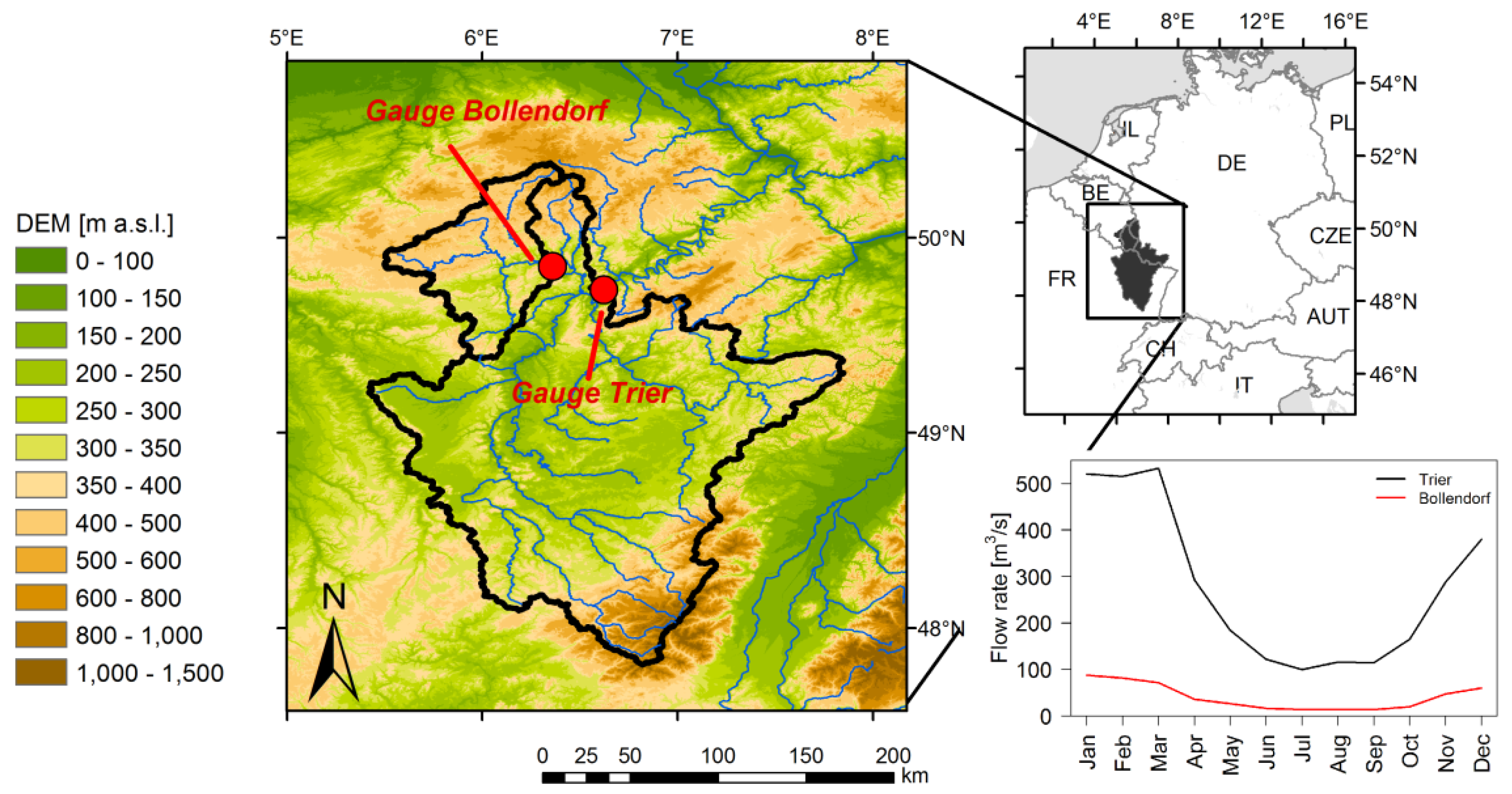
The methods are applied to daily mean flow rates at two gauges in the Moselle river basin, which is an important tributary of the river Rhine. Two different catchment sizes are considered: gauge Bollendorf located at the river Sauer with an area of 3,222 km² and a mean flow of 40 m³/s and gauge Trier at the Moselle with an area of 23,857 km² and a mean flow of 280 m³/s (see Figure 1 and

Table 1. Validation gauges, catchment area, mean flow, and maximum observed mean daily flow.

Gauge	River	Area (km2)	Mean Flow (m3/s)	Max. Flow (m3/s)
Trier	Moselle	23,857	280	3840
Bollendorf	Sauer	3213	40	823

). Both gauges show a rainfall dominated (pluvial) flow regime with maximum flow during winter and early spring and minimum flow in late summer.

2.2. Hydrological and Statistical Models

Hourly runoff simulations from two hydrological and one statistical models aggregated to daily values are used to estimate the predictive uncertainty at the two gauges: the conceptual model HBV [25], the physically based Representative Elementary Watershed model REW [26,27] and the statistical model Echo State Networks (ESN) based on artificial Recurrent Neural Networks (RNN) [28]. All models use observed meteorological data, which are spatially interpolated to the subbasins of the specific models as meteorological forcing series.

For the semi-distributed HBV model, the catchment is subdivided into four (gauge Bollendorf) and respectively 26 (gauge Trier) subbasins. These subbasins are further subdivided into hydrological response units according to land use and elevation classes. The hydrological processes for runoff generation are calculated for those HRUs on the basis of linear conceptual stores. The model estimates runoff at hourly resolution using temperature and precipitation forcing time series that have been spatially interpolated to the subbasins. The potential evapotranspiration is derived from long-term mean daily evapotranspiration values which have been corrected by the effect of actual temperature [25]. The model has been calibrated for the 1996–2007 period.

For application of the spatially-distributed REW-model, the catchment of gauge Bollendorf is subdivided into nine Representative Elementary Watersheds (REWs) and the one of gauge Trier into 85 entities. The REWs represent irregularly-shaped modelling elements for which relevant hydrological processes are identified and modelled. The unsaturated zone is further broken down into subunits based on land-use and soil type. The main governing equations are upscaled point-scale conservation equations. Physical governing equations, such as the Richards equation, are also used to describe vertical moisture diffusion through the unsaturated soil column. Hourly time series of precipitation, temperature and relative air humidity interpolated toward REWs force the model at 15 min time steps. The model was calibrated for the 1996–2011 period.

Recurrent neural networks (RNN) [29] are inspired by the information processing in biological neural networks. The processing elements represent neurons which are linked by connections. This connection topology contains feedback loops, and therefore previously received input signals are still represented in the net (i.e., implement some memory) and influence its output. Mathematically, a RNN is a dynamical system akin to a system of differential equations. RNNs are able to model the input-output behavior of dynamical systems which have states evolving over time. The same temperature and precipitation time series used for the HBV subbasins are applied as input time series to the RNN. Echo State Networks ESN [28,29] is a method designed for constructing and training large RNNs. ESNs are built in a special way, thereby ensuring the so called “Echo State property”, and then only the connections to the output nodes are computed in the training phase. This is done using regression, which is far more simple and stable than gradient-based optimization. This simplicity enables the training of large networks including thousands of internal nodes. These large nets have the capacity of learning high-dimensional dynamics of complex systems. Two ESN have been trained for each gauge for the 2000–2012 period and two flow situations: one with focus on low to mean flow and the second with focus on mean to high flows. The two outputs are combined on the basis of the specific situation reproduced by the ESNs. Each ESN had one output node (i.e., the predicted flow), 2000 internal nodes, and eight (gauge Bollendorf) and 40 (gauge Trier) input nodes, i.e., temperature and precipitation for each HBV subbasin to be considered.

The chief aim of this study is to demonstrate PU assessment using copulas rather than addressing hydrological calibration and validation strategies. Hence, model simulations are used “as is”, despite inconsistencies between different calibration and validation periods. The uncertainty processor was applied to the 1 October 2000 to 30 September 2015 period.

2.3. Copula Theory

A copula is a function that describes the dependence structure of correlated random variables independently from marginal distributions. Due to their flexibility in modelling different dependence structures, copulas are increasingly applied in multivariate analysis for flood frequency analysis, drought analysis, dam risk assessment and rainfall processing [30,31,32,33]. In hydrological forecasting, Madadgar et al. [18] and Madadgar and Moradkhani [22] applied copulas for statistical post-processing of hydrological ensemble forecasts.

For sake of brevity, we give only a short overview about copulas here. For a more detailed description of the theory, the reader is referred to [34,35,36].

After Sklar’s theorem [37] a joint multivariate probability distribution of n correlated variates X₁, X₂, X₃, …, X_n can be described through the copula function C. The copula function is a multivariate distribution function of an n-dimensional random vector on the unit cube, i.e., C: [0,1]ⁿ → [0,1], and is strictly invariant under the condition of monotonously increasing transformations of X₁, X₂, X₃, …, X_n:

$$F_{X_1,X_2,\mathrm{...},X_n}\left(x_1,x_2,\mathrm{..}{x}_n\right)=C\left[F_{X_1}\left(x_1\right),F_{X_2}\left(x_2\right),\mathrm{...},F_{X_n}\left(x_n\right)\right]=C\left(u_1,u_2,\mathrm{...},u_n\right)$$

(1)

where u₁, u₂, …, u_n ∊ [0,1] are uniformly distributed random realizations of the variates defined as $u_1=F_{X_1}\left(x_1\right)$, $u_2=F_{X_2}\left(x_2\right)$, …, $u_n=F_{X_n}\left(x_n\right)$.

The joint multivariate density function is expressed via the copula density c as follows:

$$f_{X_1,X_2,\mathrm{...},X_n}\left(x_1,x_2,\mathrm{..}{x}_n\right)=\frac{{\partial }^{n}C\left(u_1,u_2,\mathrm{...},u_n\right)}{\partial u_1\partial u_2\mathrm{...}\partial u_n}{\displaystyle \prod _{i=1}^n{f}_{X_i}\left(x_i\right)}=c\left(u_1,u_2,\mathrm{...},u_n\right){\displaystyle \prod _{i=1}^n{f}_{X_i}\left(x_i\right)}$$

(2)

2.4. Pair-Copula Construction

For the bivariate case, which models the dependency of two random variables, a large number of copulas are available [34,35]. By contrast the number of available copula functions for the multivariate case is rather limited and the applicable elliptical (Gaussian copulas, Student t copulas) and exchangeable Archimedian copulas lack the flexibility to model dependency structures of multiple heterogeneous random variables. To overcome this problem, the concept of Vine copulas has been developed [38,39,40,41]. Vine Copulas are a flexible graphical model to build multivariate copulas from a cascade of bivariate or pair-copulas. The advantage of this pair-copula construction is the decomposition of the multivariate probability density into several bivariate copulas, which can be selected independently. Vine copulas have been originally applied in the area of risk-modelling in the financial sector and more recently also in hydrology [42,43,44].

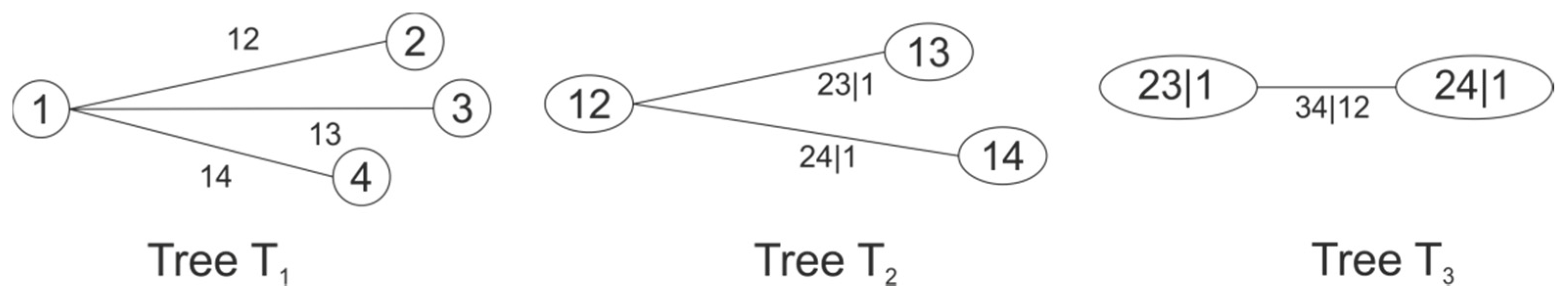
As there are a significant number of possible pair-copula constructions for high-dimensional distributions (e.g., 240 different constructions for a five-dimensional density [45]), Bedford and Cooke [39,40] introduced the graphical model, the so called Regular Vines, which help to organize possible combinations. In this application, we concentrate on the special case of C(anonical)-Vines [45], which we consider the most suitable pair-copula construction for the estimation of the PU of hydrological multi-model ensembles. All conditional random variables can be directly linked to the random variable of interest, the observation (random variable 1 in Figure 2).

Figure 2 shows the graphical representation of a four-dimensional C-Vine copula. It consists of a number of random variables n − 1 trees T, Tree T_j has n + 1 − j nodes and n − j edges. In total, the decomposition is defined by n (n − 1)/2 edges and each edge is represented by a pair-copula density. The labels of the edges represent subscript of the copula density, e.g., 13|2 denotes the copula density c_13|2(·) [39,45].

The n-dimensional density of the C-Vine copula is defined as:

$$f\left(x_1,\dots x_n\right)={\displaystyle \prod _{k=1}^{n}f\left(x_k\right){\displaystyle \prod _{j=1}^{n-1}{\displaystyle \prod _{i=1}^{n-j}{c}_{j,j+i|1,\dots ,j-1}\left[F\left(x_j|x_1,\dots ,x_{j-1}\right),F\left(x_{j+i}|x_1,\dots ,x_{j-1}\right)\right]}}}$$

(3)

with j sweeping the trees and i sweeping the edges in each tree.

The conditional distribution functions for each node in a tree are determined by sequentially applying the following equation over the previous trees:

$$F\left(x|\mathsf{\upsilon }\right)=\frac{\partial C_{x,{\upsilon }_j|{\upsilon }_{-j}}\left[F\left(x|{\upsilon }_{-j}\right),F\left({\upsilon }_j|{\upsilon }_{-j}\right)\right]}{\partial F\left({\upsilon }_j|{\upsilon }_{-j}\right)}$$

(4)

with the m-dimensional vector υ, υ_j an arbitrary element of υ and υ_-j the (m − 1)-dimensional vector υ excluding element υ_j.

When applying C-Vines, the PU of the random variable observation (random variable X₄ in Figure 2) conditional on other variables can be solved analytically by means of Equation (4). In this case, the key variable has no direct connection to the remaining variables in the most important first tree, and the dependence is only modelled indirectly in the downstream trees. Hence, it is recommended to locate the key variable at the root (variable X₁ in Figure 2) of the C-Vine copula [45]. The conditional copula density of the root variable conditional on the other variables is:

$$c_{1|2,3,\mathrm{...},n}\left(u_1|u_2,u_3,\mathrm{...},u_n\right)=\frac{c_{1,2,3,\mathrm{...},n}\left(u_1,u_2,u_3,\mathrm{...},u_n\right)}{c_{2,3,\mathrm{...},n}\left(u_2,u_3,\mathrm{...},u_n\right)}$$

(5)

As the pair-copula only “approximates” the full copula density, it is difficult to derive the lower-dimensional copula density in the denominator analytical. In this application, we calculated the copula density in the denominator by integrating c_1,2,…,n numerically over the first variable between 0 and 1 while fixing the remaining ones.

The PU of the observation y, conditional on multiple hydrological predictions ŷ, can be finally expressed via the numerical integration of Equation (5) as:

$$F\left(y|{\widehat{y}}_1,{\widehat{y}}_2,\mathrm{...},{\widehat{y}}_n\right)={\displaystyle \underset{0}{\overset{F\left(y\right)}{\int }}{c}_{1|2,3,\mathrm{...}n}\left(u_1|u_2=F\left({\widehat{y}}_1\right),u_3=F\left({\widehat{y}}_2\right),\mathrm{...},u_n=F\left({\widehat{y}}_n\right)\right)d{u}_1}$$

(6)

The selection of the pair-copula families and the parameter estimation of the C-Vine copulas is done stepwise [46]. In the selection process, the appropriate pair-copula functions are selected sequentially tree by tree as the conditional pairs of the higher order trees depend on the previous trees. The copula functions are chosen via Akaike’s Information Criteria (AIC) [47] and the canonical maximum likelihood method [48] for parameter estimation among the following options [34,35,46]: Gaussian, Student t, Gumbel, Joe, BB1, BB6, BB7, BB8 copula as well as the corresponding survival copulas (rotated by 180 degrees) of the Clayton, Gumbel, Joe, BB1, BB6, BB7, BB8. The canonical maximum likelihood method estimates the parameters of the copula function independently of the uncertain estimation of the marginal distributions, as it uses empirical probabilities to transform the sample data into the uniform variates. After selecting the copula families and estimating their parameters for all edges sequentially, the parameters of the whole C-Vine structure are optimized simultaneously by maximizing the log-likelihood of the C-Vine copula [46]. The goodness-of-fit of the pair-copulas are analyzed graphically by comparing the bivariate sample values with simulated values from the estimated copula in the copula space and for the copulas of the first tree also in the original space. Moreover, the empirical and theoretical λ-functions [49] defined as λ = v − K(v), with K(v) Kendall’s distribution of the random variable C(u₁, u₂) are also compared. In this application, the C-Vine choice and parameter estimation was performed with the R-package CDVine [46].

2.5. Marginal Distributions and Normal Quantile Transform

In most of the existing approaches for PU estimation, meta-Gaussian models are applied to describe the joint distribution between the transformed real (observed) and simulated values of the variable of interest. Simulated and observed values are transformed to the Normal space by means of the Box-Cox transformation [50], log-sinh transformation [51] and the non-parametric Normal Quantile Transform (NQT) [52,53,54], which, however, has limitations in extrapolating the relationship between the values in the Normal and real space beyond the range of the historically observed values. The non-parametric NQT relationship between the values in the real space and the values in the Normal space are calculated from the empirical probabilities and the corresponding quantiles of a standard Normal distribution. A detailed description of the application of the NQT can be found in [2]. Parametric models are needed at the tails of the NQT to extrapolate values beyond the range of available observations. Several methods have been developed to handle this problem [11,55].

In the application described here, we use parametric probability distribution functions as marginal distributions F(y) for the application of copulas according to Equation (6), and to transform the observed and predicted values y to the Normal space η when applying other PU estimation methods for inter-comparison of results (see Section 2.6):

$$\eta ={\Phi }^{-1}\left(F\left(y\right)\right)$$

(7)

with Φ⁻¹ the inverse cumulative distribution function of the standard Normal distribution.

Estimating parametric probability distributions of daily flow rates and/or water levels is often difficult, as the values arise from completely different meteorological and hydrological situations (e.g., low flows, high flows) and can in most cases not be described via one single probability distribution.

For this reason, a mixture of probability distributions has been developed to better represent the distributions of heterogeneous data [56,57,58]. Solari and Losada [58] used a mixture of probability distributions with a truncated central distribution and two generalized Pareto distributions for the maximum and minimum regimes of mean daily flow time series. The latter approach was used here to estimate the marginal distributions of the random variables.

By considering two thresholds u₁ and u₂, the probability density function (pdf) and the cumulative distribution function (cdf) of the mixed probability distribution are defined as:

$$f\left(y\right)=\{\begin{array}{cc}\begin{array}{l}{f}_m\left(y\right)F_c\left(u_1\right)\\ f_c\left(y\right)\\ f_M\left(y\right)\left[1-F_c\left(u_2\right)\right]\end{array}& \begin{array}{l}y<u_1\\ u_1\le y\le u_2\\ y>u_2\end{array}\end{array}$$

(8)

$$F\left(y\right)=\{\begin{array}{cc}\begin{array}{l}{\mathrm{F}}_m\left(y\right){\mathrm{F}}_c\left(u_1\right)\\ {\mathrm{F}}_c\left(y\right)\\ {\mathrm{F}}_c\left(u_2\right)+\left[1-F_c\left(u_2\right)\right]{\mathrm{F}}_M\left(y\right)\end{array}& \begin{array}{l}y<u_1\\ u_1\le y\le u_2\\ y>u_2\end{array}\end{array}$$

(9)

The multiplication of the lower distribution f_m(y) with F_c(u₁) and the upper distribution f_M(y) with [1 − F_c(u₂)] is required to ensure the area under the probability density graph to equal unity.

For the lower distribution a minima Generalized Pareto (GP) distribution and for the upper distribution a GP distribution is used. The type of the central distribution function can be selected independently of the upper and lower distribution as long as it is defined in the range u₁ to u₂.

The pdf of the minima GP distribution is a mirrored (y = −y) GP distribution density (defined as maxima GP distribution in the following) and the pdf and cdf are therefore defined as:

$$f_m\left(y\right)=\frac{1}{a_1}{\left[1-\frac{k_1}{a_1}\left(u_1-y\right)\right]}^{\frac{1}{k_1}-1}$$

(10)

$$F_m\left(y\right)={\left[1-\frac{k_1}{a_1}\left(u_1-y\right)\right]}^{\frac{1}{k_1}}$$

(11)

The minima GP distribution has an upper boundary u₁ for negative k: y ≤ u₁; k₁ < 0 and a lower and upper boundary for positive k: u₁ − a₁/k₁ ≤ y ≤ u₁; k₁ > 0.

The pdf and cdf of the maxima GP are defined as:

$$f_M\left(y\right)=\frac{1}{a_2}{\left[1-\frac{k_2}{a_2}\left(y-u_2\right)\right]}^{\frac{1}{k_2}-1}$$

(12)

$$F_M\left(y\right)=1-{\left[1-\frac{k_2}{a_2}\left(y-u_2\right)\right]}^{\frac{1}{k_2}}$$

(13)

The maxima GP distribution has a lower boundary u₂ for negative k: u₂ ≤ y; k₂ < 0 and a lower and upper boundary for positive k: u₂ ≤ y ≤ u₂ + a₂/k₂; k₂ > 0.

In the parameter estimation process of the mixture probability distribution, one needs to make sure that no discontinuities occur in the transition of the pdfs at the thresholds u₁ and u₂. Using the conditions f_c(y = u₁) = f_m(y = u₁) F_c(u₁) and f_c(y = u₂) = f_M(y = u₂) [1 − F_c(u₂)] the parameters a₁ and a₂ of the generalized Pareto distributions are obtained as:

$$\begin{array}{cc}{a}_1=\frac{F_c\left(u_1\right)}{f_c\left(u_1\right)};& a_2=\frac{1-F_c\left(u_2\right)}{f_c\left(u_2\right)}\end{array}$$

(14)

By defining a lower b_l and upper boundary b_u of the mixture probability distribution as an additional condition, the shape parameters k₁ and k₂ of the GP distribution result equal to:

$$\begin{array}{cc}{k}_1=\frac{a_1}{u_1-b_l};& k_2=\frac{a_2}{b_u-u_2}\end{array}$$

(15)

The remaining parameters of the mixture probability distribution left to estimate are the central distribution and the thresholds u₁, u₂. All parameters are estimated simultaneously using maximum likelihood estimation. Solari and Losada [58] used a two-parameter log-Normal distribution as central distribution function f_c. In this application, different types of central distributions (generalized Extreme Value, Logistic, generalized Logistic, Pearson3, log-Pearson3, Frechet, Gamma, Normal, log-Normal, Weibull, log-Weibull, Gumbel, Exponential, and generalized Pareto distribution [59]) were applied and the type of distribution with the best fit based on the AIC was selected.

2.6. Alternative Methods applied for PU Estimation

The results of the COpula uncertainty Processor (COP) defined in Equation (6) are compared against the results of three frequently used methods: Quantile Regression (QR) [13,14], Bayesian Model Averaging (BMA) [15,16,17,18] and Multivariate Truncated Normal (MTN) distribution as e.g., applied in the Model Conditional Processor [11]. Only a short overview of the theory of the methods is given here. For further details, we refer to the cited publications. When applying these methods, the observed and simulated values y are first transformed to the Normal variable η (model predictions are indicated by the hat symbol) and the estimated quantiles of the predictive uncertainty are back-transformed to the real space by the inverse transform. Here, the values are transformed to the Normal space by means of the same parametric mixture probability distributions used as marginal distributions in the COP via Equation (7). Hence, differences in results are attributable exclusively to the specific PU method and do not depend on the marginal distribution or the transformation method.

As done with QR, we fit separate multiple linear regression relationships for each quantile τ via optimized linear programming [60] using the model predictions as predictors. To approximate the predictive distribution, multiple quantiles need to be estimated using:

$${\eta }_{\tau }|{\widehat{\eta }}_1,{\widehat{\eta }}_2\dots ,{\widehat{\eta }}_M=a_{\tau }+{\displaystyle \sum _{i=1}^M{b}_{\tau ,i}{\widehat{\eta }}_i}$$

(16)

with a_τ, b_τ,ι the parameters of the multiple linear regression relationship and M the number of models. The R-package quantreg [61] was used for parameter estimation.

The BMA predictive distribution is a linear combination of conditional probability distributions of observation, conditional on model predictions and given that the prediction is the best possible in the ensemble. Assuming Normal conditional distributions, the BMA predictive uncertainty is:

$$f\left(\eta |{\widehat{\eta }}_1,{\widehat{\eta }}_2\dots ,{\widehat{\eta }}_M\right)={\displaystyle \sum _{i=1}^M{w}_{i}N\left(\eta |a_i+b_i{\widehat{\eta }}_i,{\sigma }_i^2\right)}$$

(17)

where w_i is the posterior probability of prediction i being the best, and M the number of models. The weights w_i are non-negative and add up to unity [15]. The conditional Normal distribution of the individual model prediction is centered on a linear dependency for the model prediction. Parameters a_i and b_i act as bias correction factors. The weights w_i and standard deviations σ_i are estimated from past model performance. We applied a two-step parameter estimation procedure: (1) maximize log-likelihood with the Expectation Maximum (EM) algorithm to estimate weights and standard deviations and (2) minimize the Continuous Ranked Probability Score (CRPS) by applying Equation (23) to optimize the estimation of the standard deviations. This procedure is implemented in the R-package ensemble BMA [62].

To consider error heteroscedasticity in PU estimation [2,11], MTN distributions can be used instead of the simple multivariate Normal distribution. Here, a combination of two MTN distributions is used. The split of the multivariate Normal space into two parts is obtained by identifying an M-dimensional hyperplane:

$$H_p={\displaystyle \sum _{i=1}^M{\widehat{\eta }}_i}=M\cdot a$$

(18)

with M the number of prediction models. The value of a is identified by minimizing the predictive variance of the upper sample. The predictive distribution for the sample above the truncation hyperplane is defined as:

$$f\left(\eta |{\widehat{\eta }}_k={\widehat{\eta }}_k^{\ast },H_P^{*}>M\cdot a\right)=N\left({\mu }_{\eta |{\widehat{\eta }}_k={\widehat{\eta }}_k^{\ast },H_P^{*}>M\cdot a},{\sigma }_{\eta |{\widehat{\eta }}_k={\widehat{\eta }}_k^{\ast },H_P^{*}>M\cdot a}^2\right)$$

(19)

with the predictive mean

$${\mu }_{\eta |{\widehat{\eta }}_k={\widehat{\eta }}_k^{\ast },H_P^{*}>M\cdot a}=\mu +{\sum }_{\eta \widehat{\eta }}{\Sigma }_{\widehat{\eta }\widehat{\eta }}^{-1}\left({\widehat{\eta }}_k^{\ast }-\widehat{\mu }\right)$$

(20)

and predictive variance

$${\sigma }_{\eta |{\widehat{\eta }}_k={\widehat{\eta }}_k^{\ast },H_P^{*}>M\cdot a}^2={\Sigma }_{\eta \eta }-{\Sigma }_{\eta \widehat{\eta }}{\Sigma }_{\widehat{\eta }\widehat{\eta }}^{-1}{\Sigma }_{\eta \widehat{\eta }}^T$$

(21)

The model parameters mean, variance and covariance matrices are estimated from the data of the upper sample. The predictive distribution of the lower sample looks similar but is defined for the values of the sample below the truncation hyperplane $H_P^{*}\le M\cdot a$. For more details see [11].

2.7. Verification

We base the verification of the predictive distributions estimated with the methods described above on the paradigm of maximizing the sharpness of the predictive distributions subject to calibration [63]. Calibration refers to the statistical consistency between the predictive distribution and observations. The percentage levels of prediction intervals should be equal to the relative frequency of the observations to lie within the corresponding quantiles of the predictive distribution. Another common term for calibration in the present context is “reliability”. Sharpness refers to the concentration of the predictive distribution. The more concentrated (“narrow” prediction intervals) the predictive distribution, the sharper the prediction.

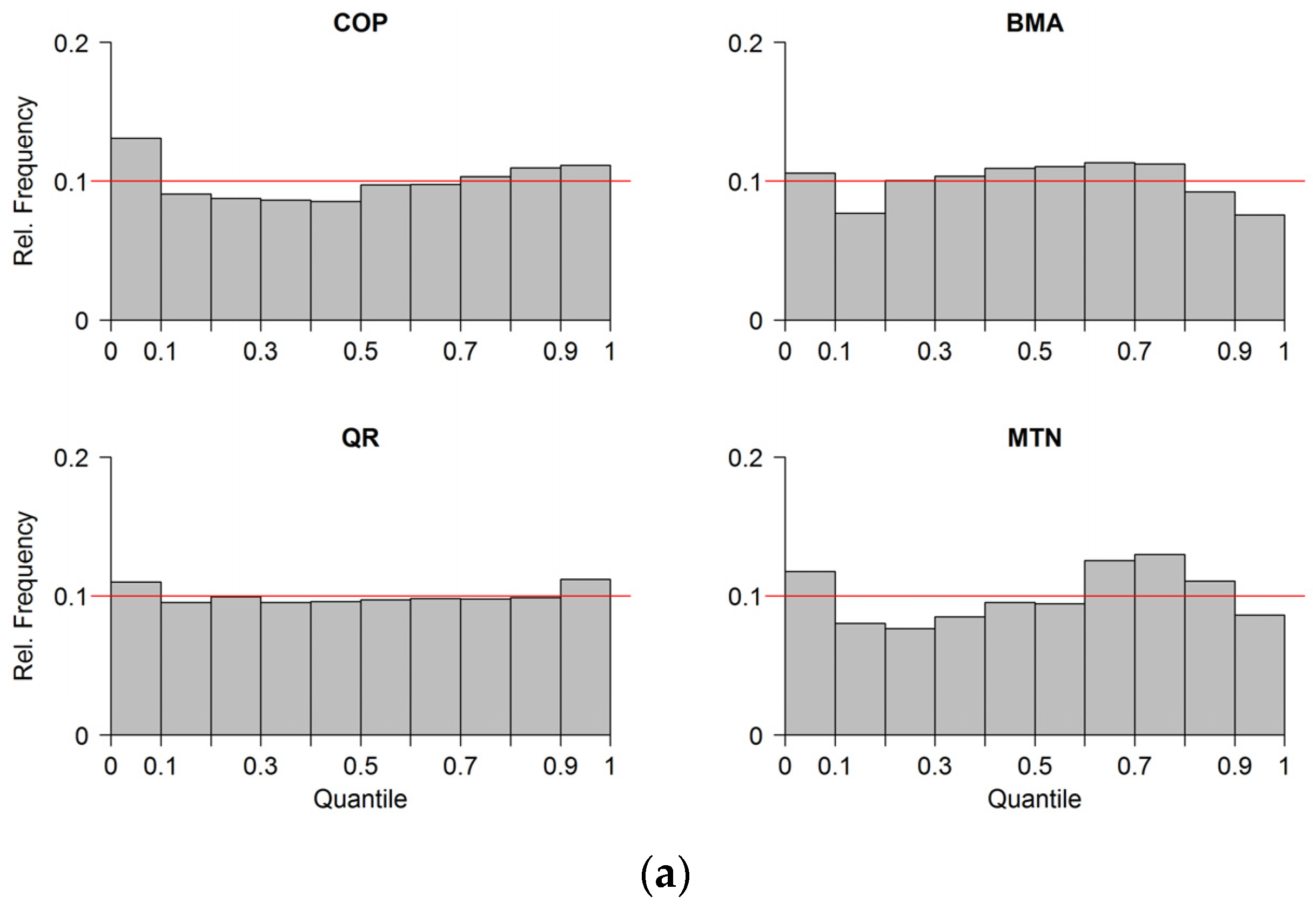
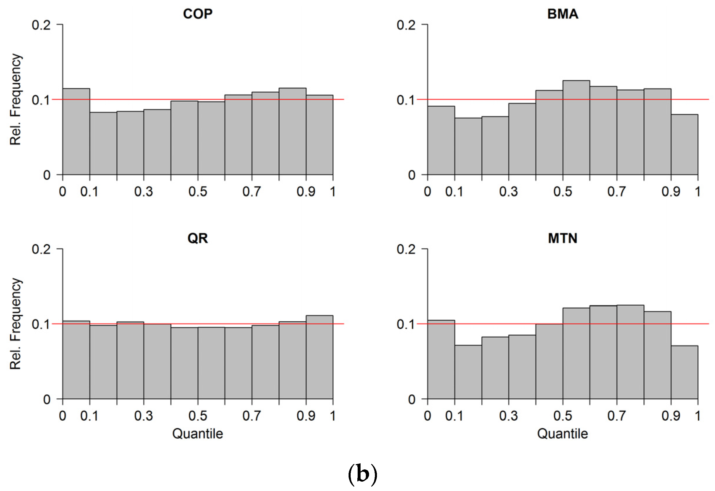
Reliability is assessed via the probability integral transform (PIT) [63]. From predictive distribution the non-exceedance probability is estimated for each value observed. These probabilities should have a uniform distribution, i.e., the observations should look like random samples from the predictive distribution. When deriving the relative frequencies of the non-exceedance probabilities for defined 10% quantile intervals, one obtains the PIT-histogram. A flat histogram indicates good calibration, whereas under-dispersion is indicated by a ∪-shape and overdispersion by a ∩-shape, respectively. Sharpness is assessed by the distribution within the 5%–95% credibility interval of each verification day. The distribution is illustrated by a modified Box-Whisker-Plot: the box represents the 25%–75% quantile, the median is the band inside the box and the whiskers represent the 5% and the 95% quantile. Outliers are not shown. Additionally, the predictive distribution is verified by the probabilistic verification measures Brier Skill Score (BSS) and the Continuous Ranked Probability Skill Score (CRPSS), two combined measures of reliability, sharpness and accuracy.

The Brier Score (BS) is a common verification measure of binary events (yes/no). It expresses the mean squared error of the probability forecast p_i, considering that observation o_i is 1 if the event occurs and 0 in its absence [21]:

$$BS=\frac{1}{n}{\displaystyle \sum _{i=\text{}1}^n{\left(p_i-o_i\right)}^2}$$

(22)

with n the number of verification days. In this application, the event is defined as the exceedance vs. non-exceedance of flow rate thresholds ranging from the 5% quantile to the 95% quantile of observed daily mean flow values.

The Continuous Ranked Probability Score (CRPS) verifies the full continuous distribution and is the squared difference between the predictive distribution F_i^f and the distribution of the observation ${F_i}^o$ [21]:

$$CRPS=\frac{1}{n}{\displaystyle \sum _{i=1}^n{\displaystyle \underset{-\infty }{\overset{\infty }{\int }}{\left[F_i{}^f\left(y\right)-F_i{}^o\left(y\right)\right]}^{2}dy}}$$

(23)

whereas the probability distribution of the observation is a cumulative-probability step function that jumps from 0 to 1 at the point where the variable y equals the observation.

The corresponding skill scores CRPSS = 1 − CRPS_FOR/CRPS_REF and BSS = 1 − BS_FOR/BS_REF are calculated from the CRPS_FOR and BS_FOR of the predictive distribution and the CRPS_REF and BS_REF of the reference forecast, for which the climatological forecast, i.e., the observed daily mean flow of the period from 1 October 2000 to 30 September 2015 is used. Due to the strong seasonality of the flow at the two gauges (see Figure 1) the CRPSS and BSS are calculated for each month separately and the climatological forecast is calculated only from the observed values of the corresponding month excluding the current month of verification. A perfect forecast has a skill score of one, negative skill score values indicate that the climatological forecast is superior to the predictive uncertainty derived from the model predictions.

The accuracy of the expected value of the predictive distribution as well as the goodness-of-fit of the deterministic model predictions is verified with the modified Kling-Gupta efficiency KGE’ and its respective components [64]:

$$KGE\prime =1-\sqrt{{\left(r-1\right)}^2+{\left(\beta -1\right)}^2+{\left(\gamma -1\right)}^2}$$

(24)

$$\rho =\frac{Cov\left(y,\widehat{y}\right)}{{\sigma }_{\widehat{y}}{\sigma }_y}$$

(25)

$$\beta =\frac{{\mu }_{\widehat{y}}}{{\mu }_y}$$

(26)

$$\gamma =\frac{C{V}_{\widehat{y}}}{C{V}_y}=\frac{{\sigma }_{\widehat{y}}/{\mu }_{\widehat{y}}}{{\sigma }_y/{\mu }_y}$$

(27)

where ρ is the Pearson correlation between the observation and prediction, β is the bias ratio, γ is the variability ratio which uses the ratio between the coefficient of variation of the prediction and the observation. All components have their optimum at unity and the KGE’ gives the lower limit of the three components [64].

The expected value of the predictive distribution is calculated as the mean of 1%-quantiles of the predictive distribution.

3. Results and Discussion

We applied the COP introduced here and the other uncertainty processors to estimate the PU of the observed daily mean flow values conditional on model predictions at two gauges located in the Moselle river basin for the 1 October 2000 to 30 September 2015 analysis period. To ensure that no flow values are simultaneously used for parameter estimation and validation of the predictive distribution, we used a Leave-One-Out Cross Validation (LOOCV) procedure. For each validation year, the parameters of the uncertainty processors were estimated from the values of the study period, by excluding the values of the validation year. In total, the parameters of each uncertainty processor were updated once per validation year.

3.1. Model Predictions

The goodness-of fit of the three model predictions is reported in

Table 2. Goodness-of-Fit (GoF) measure KGE′ and its components for the two hydrological model predictions HBV, REW and the prediction with the echo state network model ESN for the period 1 October 2000 to 30 September 2015 at the gauges Bollendorf and Trier.

GoF Measure	Bollendorf			Trier
	HBV	ESN	REW	HBV	ESN	REW
KGE′	0.85	0.78	0.75	0.83	0.87	0.85
Correlation ρ	0.94	0.89	0.89	0.95	0.95	0.89
Bias-Ratio β	1.10	0.99	1.22	0.84	1.03	1.01
CV-Ratio γ	0.91	0.80	1.05	0.95	0.88	1.10

for the whole 1 October 2000 to 30 September 2015 study period. All models are in better agreement with observations at gauge Trier, which has the seven-fold upstream catchment area of gauge Bollendorf, based on the goodness-of-fit measure modified Kling-Gupta Efficiency KGE′ and its components. From the values in the table, it is evident that the KGE′ provides the lower limit of its respective components. At both gauges, the predictions of the HBV model show significant bias, whereas the ESN model has difficulties in capturing the variability of the observations at both gauges. The REW predictions show a significant bias only at the gauge Bollendorf. Concentrating on the linear relationship between observations and predictions in terms of cross-correlations, the HBV model shows the best results at both gauges. Overall, no model outperforms the others at both gauges and for all measures.

3.2. Estimation of the Marginal Distributions

In a first step of the PU estimation using the COP (Equation (6)), the marginal distributions of the random variables need to be estimated. Mixture probability distributions (Equations (8) and (9)) have been fitted to the observed mean daily flow values as well as to the HBV, REW and ESN predictions at the two gauges.

In the parameter estimation process, a flow rate 0 m³/s was used as lower and three times the maximum rate as the upper boundary. For the distribution of the observed values, the maxima shown in Table 1 and for the distributions of the predictions the maximum values of the simulated time series 1 October 2000 to 30 September 2015 were used. The types of the central distributions have been selected based on the AIC, using the maximum likelihood method for parameter estimation.

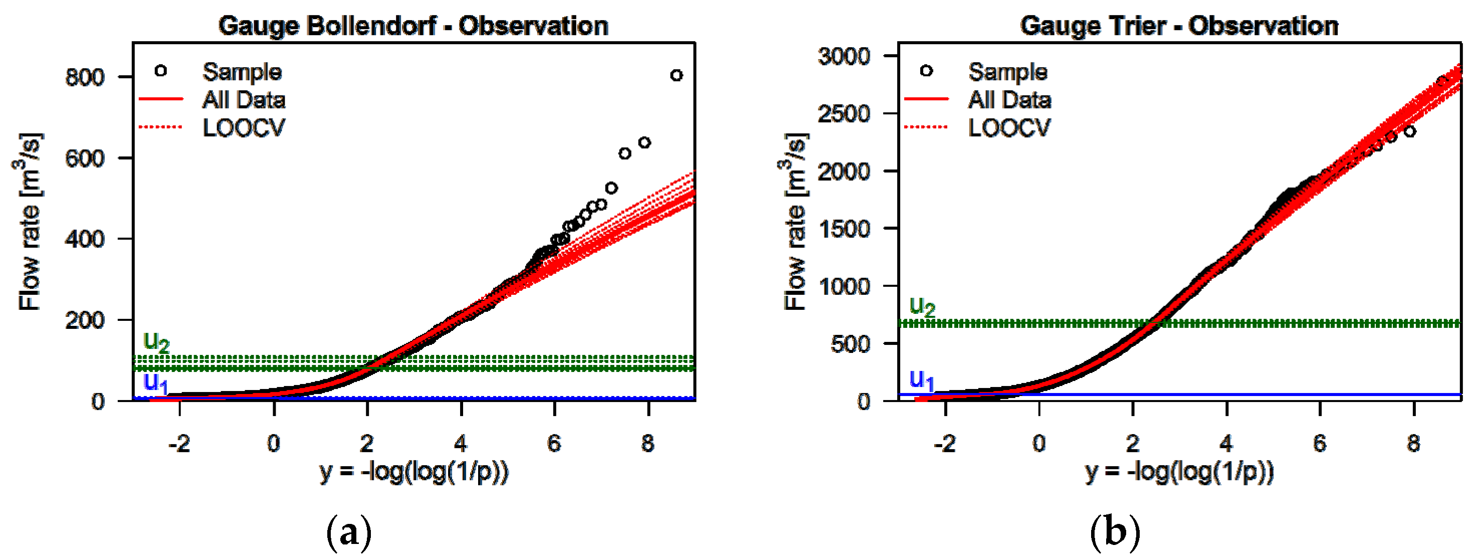
Figure 3 shows the cumulative distribution function (cdf) plots of the mixture distributions fitted to the observed daily mean flow at gauges Bollendorf and Trier and the two thresholds u₁ and u₂. At Bollendorf, the identified central distribution of the mixture distribution was the log-Pearson3 and, at Trier, the generalized Pareto distribution using all data of the 1 October 2000 to 30 September 2015 analysis period. The selection of the type of the central distribution is relatively stable. When using the LOOCV subsample sets at gauge Bollendorf, the same distribution (log-Pearson3) was identified 10 times out of 15 subsamples and, at gauge Trier, the same distribution (generalized Pareto distribution) was identified for all subsamples. The variability of the fitted distributions and the two thresholds u₁ and u₂ for the different subsamples in the LOOCV are shown in Figure 3 as dotted lines.

At gauge Bollendorf, several values are above the theoretical distribution at the upper tail. This is due to the fact that the highest observed flood in the last 56 years at gauge Bollendorf falls within the 15-year study period. The daily flow rates of this flood have therefore a lower probability of occurrence than the empirical probabilities shown in Figure 3. The overall fit of the modeled distributions is satisfactory on visual inspection. For the mixture distributions of the individual model predictions, other central distributions have been identified in the selection process.

3.3. C-Vine Copula Selection and Estimation

In the next step of the COP estimation, the C-Vine structure needs to be defined. As the central variate 1 in Figure 2, we chose the “observations” because it is directly linked to the other variables in the first tree. The other random variables in Figure 2 are HBV (2); ESN (3); and REW (4). Other combinations of variates 2–4 would lead to slightly different but overall similar results. The bivariate copula families have been selected based on the AIC using the canonical maximum likelihood method for parameter estimation.

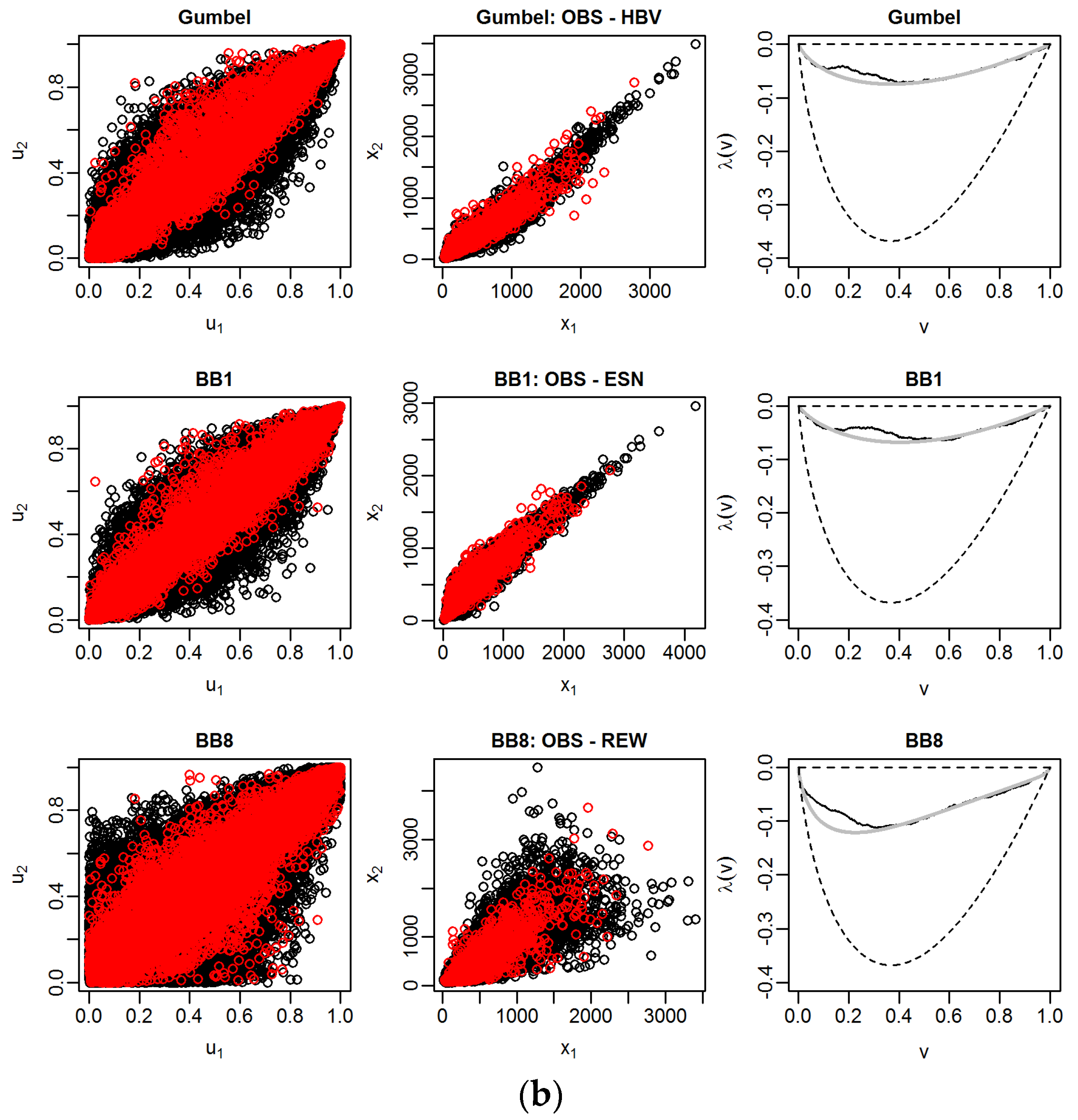
The scatter plots in the second column of Figure 4 show that all bivariate random samples have a different dependence structure but all of them indicate an upper tail dependence, implying that the two variates behave similarly at the upper tail of the distribution. Hence, we use only bivariate copulas, which allow modeling upper tail dependence. The frequently used Clayton and Frank copulas are not selected because of their poor capability to represent upper tail dependence.

Figure 4 illustrates the goodness-of-fit of the estimated bivariate copulas of the most important first tree of the C-Vine copula at both gauges using all data of the 1 October 2000 to 30 September 2015 analysis period.

In the first column, the scatter plots of random pairs chosen from the selected pair-copulas with the sample values in the copula space are compared, while in the second one the back-transformed values using marginal distributions are compared in the real space. The size of the respective random samples is 10 times the size of the bivariate sample. Comparing simulated and sample values in the two scatter plots, we can conclude that the fitted copulas are able to capture the dependence structure of the bivariate samples. In the third column the empirical λ-functions (black) of the bivariate samples and the theoretical λ-functions (grey) of the estimated pair-copulas are shown. The dashed lines below and above are bounds corresponding to independence (lower line) and comonotonicity (λ = 0), i.e., perfect positive dependence, respectively. As the empirical λ-functions are near the line of co-monotonicity, there is a strong dependence between all considered combinations of the random variables. Overall, the fitted copulas show good agreement with empirical values. We note that for nearly all pair-copulas estimated at both gauges, there is a deviation between theoretical and empirical functions when the random variable v = C (u₁, u₂) takes on values between 0.1 and 0.3. No theoretical copula function exists, which is able to capture the irregularity in the λ-function of the bivariate sample data present at both gauges.

Table 3. Pair-copula families of the C-Vine identified using all data and LOOCV (validation year as identifier) at gauge Trier.

LOOCV	Tree 1			Tree 2		Tree 3
Sample	CObs,HBV	CObs,ESN	CObs,REW	CHBV,ESN|Obs	CHBV,REW|Obs	CESN,REW|Obs,HBV
All Data	Gumbel	BB1	BB8	Student t	Student t	Student t
2001, 2014	Gumbel	BB1	BB8	Student t	Student t	Independence
2002, 2004	BB1	Student t	BB8	Student t	Student t	Independence
2003, 2005, 2006, 2007, 2008, 2009, 2010, 2013, 2015	Gumbel	BB1	BB8	Student t	Student t	Student t
2011	Gumbel	Student t	BB8	Student t	Student t	Independence
2012	BB1	BB1	BB8	Student t	Student t	Independence

shows the identified pair-copula families using all data and the LOOCV subsample sets for the gauge Trier. It is evident that the identification of the pair-copulas is relatively stable as the same copulas are identified for nearly all subsamples. In the LOOCV procedure, these copula families are used to estimate the PU.

3.4. Verification

The quality of the estimated predictive distributions using the COP (Equation (6)) and results of BMA, QR and MTN distribution (Equations (16), (17) and (19)) are verified and compared below. Based on the verification metrics presented before, the measures sharpness, reliability and accuracy of the estimated predictive distributions are verified and compared for the whole study period. All verification results are based on the estimated predictive distributions from the LOOCV strategy. Hence, no values are used simultaneously for parameter estimation and verification.

In Figure 5, the reliability of the estimated predictive distributions is depicted as Probability Integral Transform (PIT)-histograms. For the predictive distribution estimated with the COP, the number of observations in the lower quantile ranges (10%–40%) are slightly below and the number of observation in the lowest quantile range (0%–10%) are above the optimal value of 10% at both gauges. The shape of the COP PIT-histogram at both gauges could be an indication of a small negative bias. The shapes of the PIT-histograms of BMA and MTN indicate over-dispersion at both gauges, which suggests that the estimated variance of the distributions is too large. The highest reliability indicated by the flat shape of the histogram is that of the QR approach, which is reasonable since the parameters of QR quantiles are optimized based on reliability. Moreover, in QR, the number of fitted parameters is considerably higher than that of the other methods. For each quantile, four parameters need to be estimated. This means that, in total, 36 parameters have been estimated for the nine quantiles 10%–90% used for reliability verification. Despite small overall differences, we conclude that all estimated predictive distributions can be considered reliable with outperformance of COP and QR.

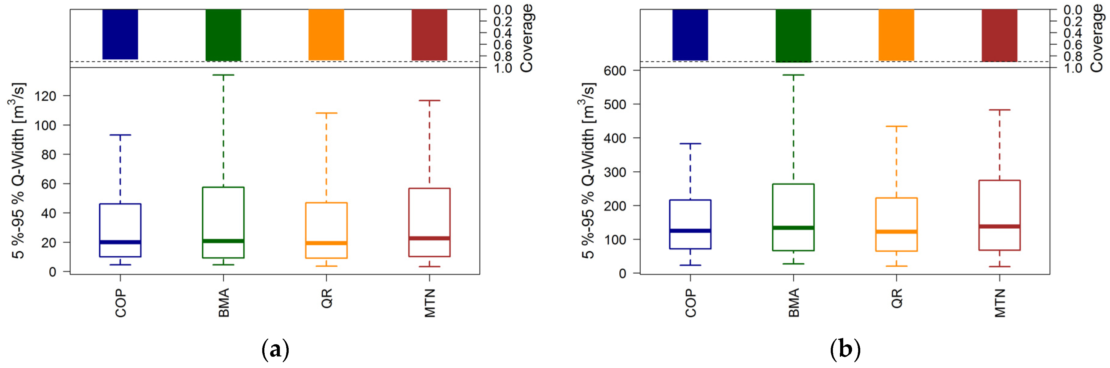
Verification of reliability as well as calibration is only meaningful in combination with the assessment of sharpness, which is an attribute of the prediction alone. For sharpness assessment of the predictive distributions, the width of the 5%–95% quantile range is calculated for each verification day. The smaller the widths of the quantile range the sharper and more adherent the predictive distribution is. Figure 6 shows important quantiles of the distribution of the widths as modified box plots.

The upper part of Figure 6 illustrates the coverage, which measures the proportion of observations that fall within the 5%–95% quantile range. In principle, 90% of observations should fall within this interval, which is the case in all applied methods. QR and COP provide sharper predictions than MTN and BMA. Other quantile ranges analyzed (10%–90%, 25%–75%, not shown here) show similar tendencies.

To assess the predictive performance of the estimated distributions for different runoff situations (low flow, mean flow, high flow), we calculate the Brier Skill score for the non-exceedance probabilities of different flow rate thresholds, ranging from the 5%–95% quantile of the observations. Figure 7 shows the BSS values at the two gauges.

At both gauges, all methods show similar skill in terms of BSS for all flow rate thresholds. At gauge Bollendorf, QR and MTN show a higher skill for higher quantiles and a lower skill for smaller quantiles than COP and BMA. Overall, the predictive performance of all methods is comparable at both gauges. We note a local maximum at the 25% quantile of all methods at both gauges. For larger quantiles, the BSS decreases and then rises again with threshold values higher than the 50% quantile.

This effect could correspond to the irregularities observed in the empirical λ-function of the bivariate samples at both gauges in Section 3.3 related to the prediction performance of the applied prediction models, which cannot be captured by the theoretical functions.

Table 4. Deterministic Goodness-of-Fit (Gof) measure KGE′ and its components of the expected values of the predictive distributions estimated with the COpula uncertainty Processor (COP), Bayesian Model Averaging (BMA), Quantile Regression (QR), Multivariate Truncated Normal (MTN) distribution and the probabilistic skill score CRPSS of the predictive distributions for the gauges Bollendorf and Trier.

GoF Measure	Bollendorf				Trier
	COP	BMA	QR	MTN	COP	BMA	QR	MTN
KGF′	0.91	0.90	0.90	0.93	0.96	0.96	0.96	0.96
Correlation ρ	0.94	0.94	0.94	0.94	0.97	0.97	0.97	0.97
Bias-Ratio β	1.03	1.05	0.99	1.00	1.00	1.01	1.00	1.00
CV-Ratio γ	0.95	0.94	0.92	0.95	0.99	0.98	0.97	0.98
CRPSS	0.61	0.62	0.63	0.63	0.71	0.71	0.72	0.72

shows the probabilistic verification measure CRPSS together with the deterministic goodness-of-fit measure KGE′ and its components. These are indicators of the accuracy of the expected value of the predictive distributions. Noting that the CRPS is the integral of the BS over all threshold values, the CRPSS values in Table 4 confirm the results of the BSS analysis above. At both gauges, the skill scores of the different methods are similar. A comparison of the results with goodness-of-fit measures for model predictions in Table 2 reveals that all methods lead to a significant improvement of model predictions in deterministic terms. By focusing on the bias ratio, it becomes evident that the post-processing methods also act as bias-correction. At gauge Trier, also the variability of the expected value of the predictive distributions is very similar to that of observations. In general, all methods perform similarly based on the verification measures in Table 4 with no particular method clearly outperforming the other.

To highlight the effect of different model ensemble combinations on PU estimation, we show the verification results of the predictive distribution at gauge Trier using COP for different model combinations in

Table 5. Deterministic Goodness-of-Fit (GoF) measure KGE′ and its components of the expected values of the predictive distributions estimated with the copula uncertainty processor with different combinations of model predictions and the probabilistic skill score CRPSS of the predictive distributions for the gauge Trier.

GoF Measure	HBV REW ESN	HBV	ESN	REW	HBV ESN	HBV REW	ESN REW
KGE′	0.96	0.95	0.95	0.86	0.96	0.95	0.96
Correlation ρ	0.97	0.95	0.96	0.90	0.96	0.96	0.96
Bias-Ratio β	1.00	1.00	1.00	1.01	1.00	1.00	1.00
CV-Ratio γ	0.99	0.98	0.97	0.90	0.99	0.98	0.97
CRPSS	0.71	0.64	0.66	0.49	0.70	0.66	0.69

. It is clear that the combination HBV-ESN and ESN-REW performs similarly compared to the case in which all three models are used. Adding another model prediction improves the results only marginally. When comparing the results of only HBV against the HBV-REW combination, there is no significant increase in performance, implying that the REW model prediction does not add information with respect to HBV. On the other hand, the performance increases considerably when adding the ESN model to either HBV or REW, indicating that the completely different type of model structure, which is of statistical black-box type, contains complementary information.

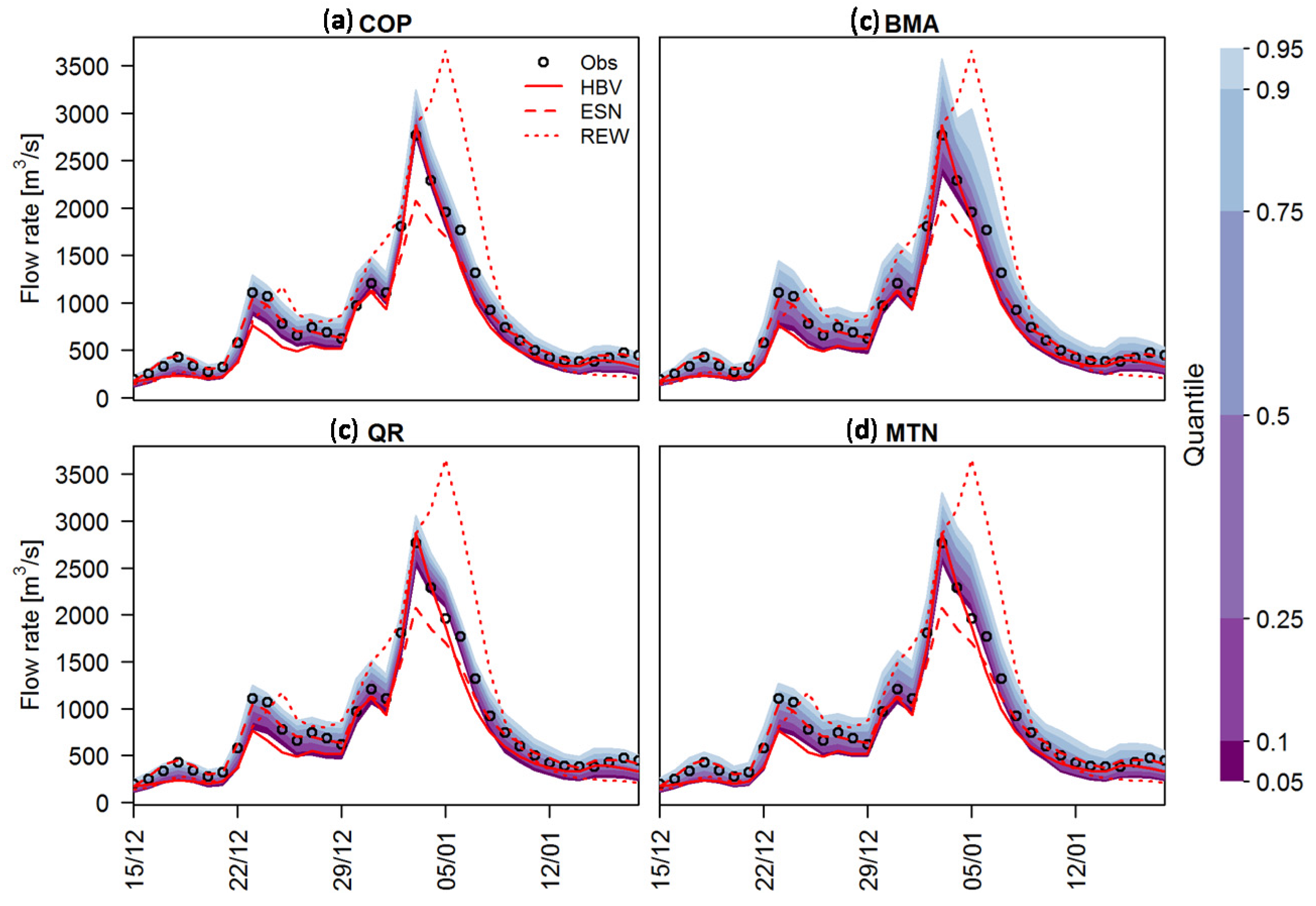
Figure 8 illustrates the uncertainty bands of the different methods applied for the winter 2002/2003 flood at gauge Trier. The REW model overestimates the flood peak, while ESN underestimates it. In this case, the HBV prediction represents the flood event almost perfectly. Besides the large differences between individual model predictions, the observed values fall well within the 5%–95% uncertainty range for all PU methods applied. The uncertainty bandwidths show the PU densities of QR and COP are sharper with respect to those of the other two methods. The wider uncertainty bands of BMA and MTN confirm the results of the sharpness verification. In summary, we conclude that all methods provide a satisfactory PU estimate for this event.

4. Conclusions

The assessment of predictive uncertainty (PU) has become increasingly important in hydrological forecasting over recent years. For this purpose, a variety of methods have been developed and applied to estimate the PU of variables of interest, conditional on hydrological model predictions. In this paper, we introduced a COpula uncertainty Processor (COP), which uses the concept of pair-copula construction to model the multivariate distribution of observation and model predictions. It allows to adequately model different dependence structures among random variables. For the required estimation of the marginal distributions of the variables, we apply mixture probability distributions, given that the flow rates depend on particular hydro-meteorological situations.

We apply the COP to the estimation of the PU for a hydrological and statistical multi-model ensemble at the gauges Bollendorf and Trier in the Moselle river basin. Predictions by the models HBV and REW with conceptual and process-based representation, respectively, as well as the artificial recurrent neural network model Echo State Networks (ESN) serve as random predictors for conditioning PU estimation.

The verification of the quality of the predictive distribution estimated with the COP and the comparison with the results of three other uncertainty processors—BMA (1); QR (2); and MTN (3)—reveals that the COP is very well suitable to estimate the PU. Especially in terms of sharpness, the performances of the methods show differences. The predictive distributions of the COP and the QR are considerably sharper than BMA and MTN. The wider uncertainty bands of the BMA can be explained by use of constant variance for the predictive distributions of individual models, which cannot account for heteroscedasticity of the error variance, and the superposition of the predictive distributions. The larger the differences between the individual model predictions the wider the uncertainty distribution. Results of the sharpness verification are confirmed in the reliability verification via the “Probability Integral Transform” (PIT)-Histogram. Both PIT-Histograms of MTN and BMA indicate overdispersion, which means that the estimated variance of the PU distribution is too large. Due to the calibration of a linear regression model for each quantile, the QR approach leads to best results in terms of reliability verification. This advantage is simultaneously the most significant drawback of the approach because of the large number of fitting parameters required and therefore potentially lower robustness. In summary, the COP provides sharp and yet reliable predictive distributions and considerably more parsimonious than the similarly performing QR. Depending on the selected bivariate copula families, 12 parameters need to be estimated at most for the PU assessment, conditional on three model predictions. Due to the construction of the multivariate probability by independent selected pair-copulas, COP is a flexible and robust approach to estimate the PU of the observation conditional on several model predictions with heterogeneous dependence structures.

Comparison of the effects of different combinations of the hydrological and statistical multi-model ensemble on PU estimation revealed that the results are significantly improved when the purely statistical model was added to the mix of hydrological models, whereas the two deterministic hydrological models hold similar information about the PU. Hence, different kinds of models should be considered in a multi-model approach with the aim to maximize the information content for PU assessment.

In future work, the presented pair-copula approach will be applied to estimate the predictive distribution of deterministic and hydro-meteorological ensemble forecasts for individual forecast values as well as to the multi-temporal case to analyze temporal dependencies between consecutive forecast values.

As the error structure of hydrological model predictions and forecasts is strongly event-dependent—i.e., the model error structure in modeling snowmelt is very different from modelling heavy rainfall events—we aim at using different copula models estimated for particular hydrological events. In this context, the PU estimation will also be made dependent on the specific event type to be analyzed.