
Hydrological Evaluation of Lake Chad Basin Using Space Borne and Hydrological Model Observations

Abstract
:1. Introduction
2. Materials and Methods
2.1. Terrestrial Water Storage (TWS) from GRACE
2.2. Lake Height from Altimetry
2.3. Soil Moisture from GLDAS
2.4. Groundwater Estimates from the WaterGap Hydrological Model
2.5. Data Processing
2.5.1. Variability in TWS and Lake Height
- Cycle-subseries smoothing: series are built for each seasonal component, and smoothed separately.
- Low-pass filtering of smoothed cycle-subseries: the subseries are put together again, and smoothed.
- Detrending of the seasonal series.
- Deseasonalizing the original series, using the seasonal component calculated in the previous steps; and Smoothing the deseasonalized series to get the trend component.
- : The number of observations in each seasonal cycle, = 12 months (yearly periodicity with monthly data);
- : The number of passes through the inner loop (usually set to equal one or two) = 1 month;
- : The number of robustness iterations of the outer loop (Values qual one or two) = po robustness while a zero value has no robustness iteration) = 5 months;
- : The span of the loess window for the low-pass filter (computed as the next odd number to ) = 13 months;
- : The smoothing parameter for the seasonal component, = 12 months (seasonal length is same as the periodic length);
- : The smoothing parameter for the trend component, = 22 months.
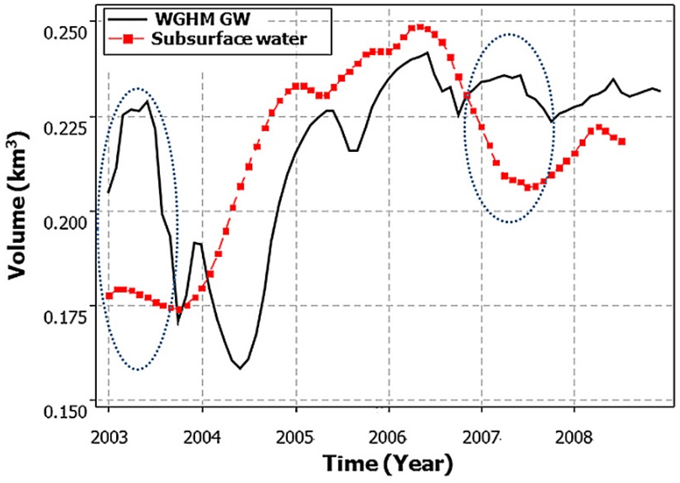
2.5.2. Subsurface Water Volume Change
3. Results and Discussions
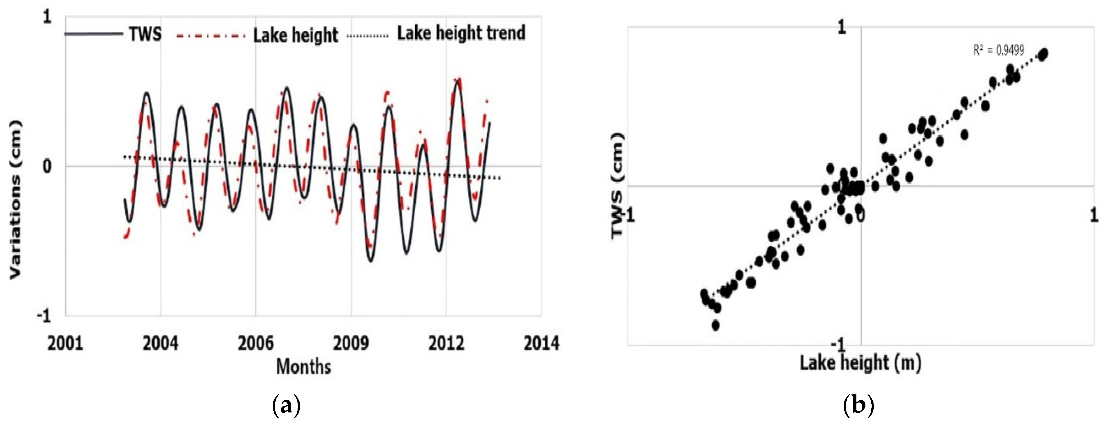
3.1. TWS and Altimetry Lake Height
3.2. TWS and Rainfall
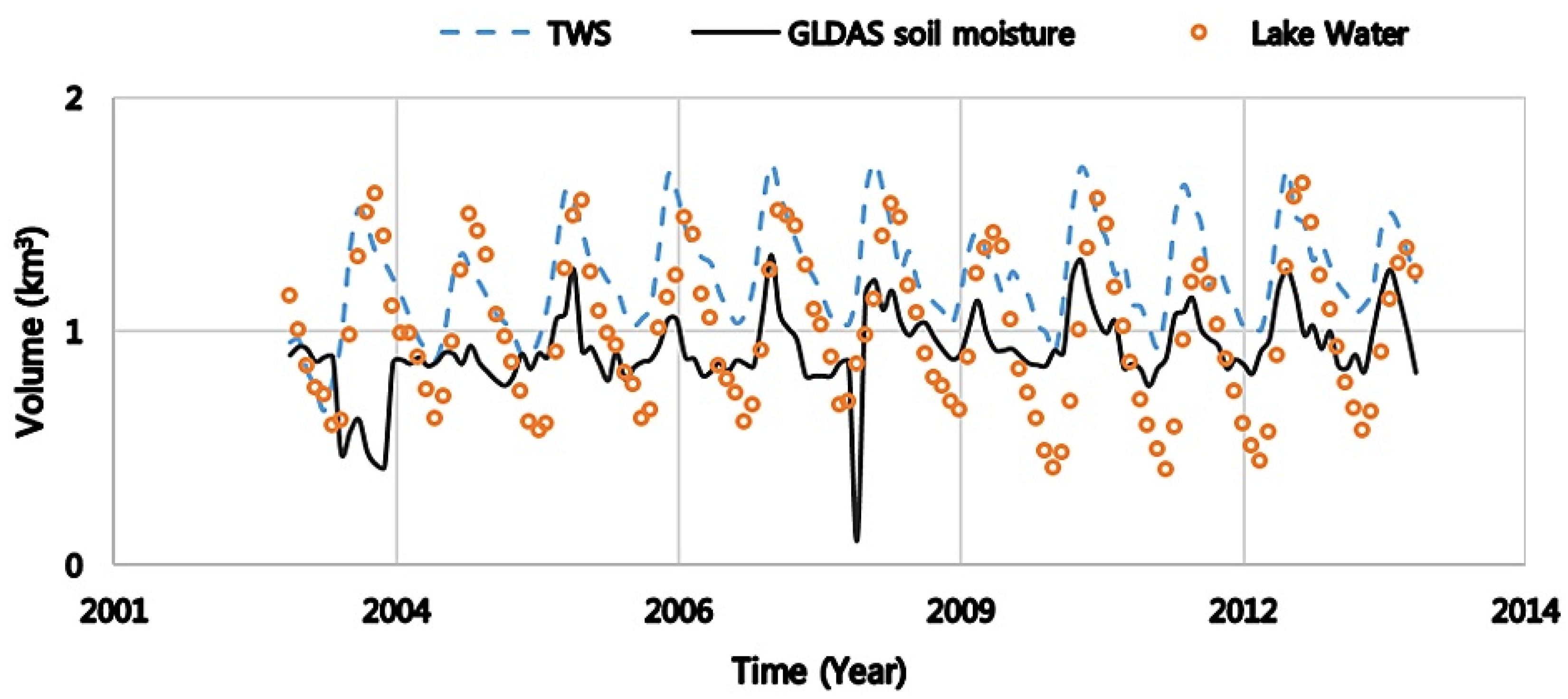
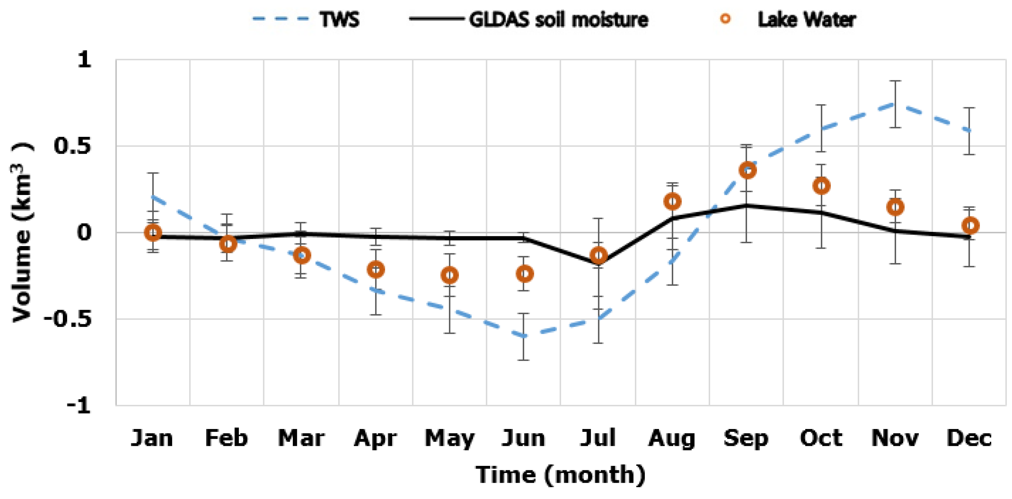
3.3. TWS and Soil Moisture
4. Conclusions
Acknowledgments
Author Contributions
Conflicts of Interest
References
- Swenson, S.; Wahr, J. Monitoring the water balance of Lake Victoria, East Africa, from space. J. Hydrol. 2009, 370, 163–176. [Google Scholar] [CrossRef]
- Allen, R.; Joseph, J.; Kevin, L.; Ahjond, S. Adaptive management for a turbulent future. Environ. Manag. 2011, 92, 1339–1345. [Google Scholar] [CrossRef] [PubMed]
- Leblanc, M.; Leduc, C.; Razack, M.; Lemoalle, J.; Dagorne, D.; Mofor, L. Applications of remote sensing and GIS for groundwater modelling of large semiarid areas: Example of the Lake Chad Basin, Africa. IAHS Publ. 2003, 278, 186–192. [Google Scholar]
- Rodell, M.; Houser, P.R.; Jambor, U.; Gottschalck, J.; Mitchell, K.; Meng, C.-J.; Arsenault, K.; Cosgrove, B.; Radakovich, J.; Bosilovich, M.; et al. The global land data assimilation system. Am. Meteorol. Soc. 2004, 85, 381–394. [Google Scholar] [CrossRef]
- Boronina, A.; Ramillien, G. Application of AVGRR imagery and GRACE measurements for calculation of actual evapotranspiration over the Quaternary aquifer (Lake Chad basin) and validation of groundwater models. Hydrol. J. 2008, 348, 98–109. [Google Scholar] [CrossRef]
- Leblanc, M.; Favreau, G.; Tweed, S.; Leduc, C.; Razack, M.; Mofor, L. Remote sensing for ground water modelling in large semiarid areas: Lake Chad basin, Africa. Hydrol. J. 2007, 15, 97–100. [Google Scholar]
- Gao, H.; Bohn, T.J.; Podest, E.; McDonald, K.C.; Lettenmaier, D.P. On the causes of the shrinking of Lake Chad. Environ. Res. Lett. 2011, 6, 034021. [Google Scholar] [CrossRef]
- Singh, A.; Diop, S.; M’mayi, P.L. Africa’s Lakes: Atlas of Our Changing Environment (Nairobi: UNEP). Available online: www.unep.org/dewa/AfricaAfricaAtlas/ (accessed on 10 May 2016).
- Campbell, R.W. Earthshots: Satellite Images of Environmental. Available online: http://earthshots.usgs.gov/ (accessed on 10 May 2016).
- Coe, M.T.; Foley, J.A. Human and natural impacts on the water resources of the Lake. Geophys. Res. Atmos. 2001, 106, 3349–3356. [Google Scholar] [CrossRef]
- Birkett, C.M. Synergistic remote sensing of Lake Chad: Variability of basin inundation. Remote Sens. Environ. 2000, 72, 218–236. [Google Scholar] [CrossRef]
- Churchill, O.; Belay, D.; Sium, G. Characteristics of Lake Chad Level Variability and Links to ENSO, precipitation and river discharge. Sci. World J. 2014, 13, 145893. [Google Scholar]
- Li, K.Y.; Coe, M.T.; Ramankutty, N.; De Jong, R. Modeling the Hydrological Impact of Land-Use Change in West Africa. J. Hydrol. 2007, 337, 258–268. [Google Scholar] [CrossRef]
- Li, B.; Rodell, M.; Zaitchik, B.F.; Reichle, R.H.; Koster, R.D.; Tonie, M.A. Assimilation of Grace Terrestrial Water Storage into a Land Surface Model: Evaluation and Potential Value for Drought Monitoring in Western and Central Europe. J. Hydrol. 2012, 446–447, 103–115. [Google Scholar] [CrossRef]
- Le Coz, M.; Delclaux, F.; Genthon, P.; Favreau, G. Assessment of Digital Elevation Model (Dem) Aggregation Methods for Hydrological Modeling: Lake Chad Basin, Africa. Comp. Geosci. 2009, 35, 1661–1670. [Google Scholar] [CrossRef]
- Leblanc, M.; Favreau, G.; Maley, J.; Nazoumou, Y.; Leduc, C.; Stagnitti, F.; van Oevelen, P.; Delclaux, F.; Lemoalle, J. Reconstruction of Megalake Chad using Shuttle Radar Topographic Mission data. Palaeogeogr. Palaeoclimatol. Palaeoecol. 2006, 239, 16–27. [Google Scholar] [CrossRef]
- Leblanc, M.; Razack, M.; Dagorne, D.; Mofor, L.; Jones, C. Application of Meteosat thermal data to map soil infiltrability in the central part of the Lake Chad basin, Africa. Geophys. Res. Lett. 2003, 30. [Google Scholar] [CrossRef]
- Coe, M.T.; Birkett, C.M. Calculation of river discharge and prediction of lake height from satellite radar altimetry: Example for the Lake Chad basin. Water Resour. Res. 2004, 40. [Google Scholar] [CrossRef]
- Isiorho, S.A.; Matisoff, G. Groundwater seepage and its implication on the water resources planning and management in the Chad Basin. Water Resour. Res. 1989, 1, 210–215. [Google Scholar]
- Isiorho, S.A.; Matisoff, G. Groundwater recharge from Lake Chad. Limnol. Oceanogr. 1990, 35, 931–938. [Google Scholar] [CrossRef]
- Leduc, C.; Sabljak, S.; Taupin, J.D.; Marlin, C.; Favreau, G. Estimation de la recharge de la nappe quaternaire dans le Nord-Ouest du bassin du lac Tchad (Niger oriental) à partir de mesures isotopiques. Earth Planet. Sci. Lett. 2000, 330, 355–361. [Google Scholar] [CrossRef]
- Goni, I.B. Tracing stable isotope values from meteoric water to groundwater in the southwestern part of the Chad basin. Hydrogeol. J. 2006, 14, 742–752. [Google Scholar] [CrossRef]
- Ngounou, N.B.; Jacques, M.; Jean, S.R. Groundwater Recharge from Rainfall in the Southern Border of Lake Chad in Cameroon. World App. Sci. J. 2007, 2, 125–131. [Google Scholar]
- Lemoalle, J.; Leblanc, M.; Bader, J.C.; Tweed, S.; Mofor, L. Thermal remote sensing of water under flooded vegetation: New observations of inundation patterns for the Small Lake Chad. Hydrol. Res. 2011, 404, 87–98. [Google Scholar]
- Becker, M.; LLovel, W.; Cazenave, A.; Guntner, A.; Crétaux, J.F. Recent hydrological behaviour of the East African great lakes region inferred from GRACE, satellite altimetry and rainfall observations. Comptes Rendus Geosci. 2010, 342, 223–233. [Google Scholar] [CrossRef]
- Jean-Paul, B.; Jacques, H.; Caroline, D.L. Retrieval of Large-Scale Hydrological Signals in Africa from GRACE Time-Variable Gravity Fields. Pure Appl. Geophys. 2012, 169, 1373–1390. [Google Scholar]
- Milzow, C.; Krogh, P.E.; Bauer-Gottwein, P. Combining satellite radar altimetry, SAR surface soil moisture and GRACE total storage changes for hydrological model calibration in a large poorly gauged catchment. Hydrol. Earth Syst. Sci. 2011, 15, 1729–1743. [Google Scholar] [CrossRef] [Green Version]
- Hassan, A.A.; Jin, S. Lake level change and total water discharge in East Africa Rift Valley from satellite-based observations. Global Planet Change 2014, 117, 79–90. [Google Scholar] [CrossRef]
- Tapley, B.D.; Bettadpur, S. The gravity recovery and climate experiment: Mission overview and early results. Geophys. Res. Lett. 2004, 31. [Google Scholar] [CrossRef]
- Wahr, J.; Swenson, S.; Zlotnicki, V.; Velicogna, I. Time-variable gravity from GRACE: First results. Geophys. Res. Lett. 2004, 31. [Google Scholar] [CrossRef]
- Swenson, S.; Chambers, D.; Wahr, J. Estimating geocenter variations from a combination of GRACE and ocean model output. J. Geophys. Res. Solid Earth 2008, 113. [Google Scholar] [CrossRef]
- Rodell, M.; Velicogna, I.; Famiglietti, J.S. Satellite-based estimates of groundwater depletion in India. Nature 2009, 460, 999–1002. [Google Scholar] [CrossRef] [PubMed]
- Lee, S.I.; Kim, J.S.; Lee, S.K. Estimation of average terrestrial water storage changes in the Korean Peninsula using GRACE satellite gravity data. J. Korea Water Resour. Assoc. 2012, 8, 805–814. [Google Scholar] [CrossRef]
- Lee, S.I.; Seo, J.Y.; Lee, S.K. Validation of terrestrial water storage change estimates using hydrologic simulation. J. Water Resour. Ocean Sci. 2014, 4, 5–9. [Google Scholar] [CrossRef]
- Henry, C.M.; Allen, D.M.; Huang, J. Groundwater storage variability and annual recharge using well-hydrograph and GRACE satellite data. Hydrogeol. J. 2011, 19, 741–755. [Google Scholar] [CrossRef]
- Joseph, L.A.; Sharifi, M.A.; Ogonda, G.; Wickert, J.; Grafarend, E.W.; Omulo, M.A. The Falling Lake Victoria Water Level: GRACE, TRIMM and CHAMP Satellite Analysisof the Lake Basin. Water Resour. Manag. 2008, 22, 775–796. [Google Scholar]
- Song, C.; Huang, B.; Ke, L. Modeling and analysis of lake water storage changes on the Tibetan Plateau using multi-mission satellite data. Remote Sens. Environ. 2013, 135, 25–35. [Google Scholar] [CrossRef]
- Longuevergne, L.; Wilson, C.R.; Scanlon, B.R.; Crétaux, J.-F. GRACE water storage estimates for the Middle East and other regions with significant reservoir and lake storage. Hydrol. Earth Syst. Sci. 2013, 17, 4817–4830. [Google Scholar] [CrossRef] [Green Version]
- Tourian, M.J.; Elmi, O.; Chen, Q.; Devaraju, B.; Roohi, Sh.; Sneeuw, N. A spaceborne multisensor approach to monitor the desiccation of Lake Urmia in Iran. Remote Sens. Environ. 2015, 156, 349–360. [Google Scholar] [CrossRef]
- NASA MEaSUREs Program. Available online: http://grace.jpl.nasa.gov (accessed on 10 May 2016).
- Crétaux, J.-F.; Birkett, C.M. Lake studies from satellite radar altimetry. Comptes Rendus Geosci. 2006, 338, 1098–1112. [Google Scholar] [CrossRef]
- Kouraev, A.V.; Semovski, S.V.; Shimaraev, M.N.; Mognard, N.M.; Légresy, B.; Remy, F. Observations of Lake Baikal ice from satellite altimetry and radiometry. Remote Sens. Environ. 2007, 108, 240–253. [Google Scholar] [CrossRef]
- Kropacek, J.; Braun, A.; Kang, S.C.; Feng, C.; Ye, Q.H.; Hochschild, V. Analysis of lake level changes in Nam Co in central Tibet utilizing synergistic satellite altimetry and optical imagery. Int. J. Appl. Earth Obs. Geoinf. 2012, 17, 3–11. [Google Scholar] [CrossRef]
- Duan, Z.; Bastiaanssen, W.G.M. Estimating water volume variations in lakes and reservoirs from four operational satellite altimetry products and satellite imagery data. Remote Sens. Environ. 2013, 134, 403–416. [Google Scholar] [CrossRef]
- Goddard Earth Sciences Data and Information Services Center. Available online: http://grace.jpl.nasa.gov (accessed on 10 May 2016).
- Döll, P.; Kaspar, F.; Bernhard, L. A global hydrological model for deriving water availability indicators: Model tuning and validation. J. Hydrol. 2003, 270, 105–134. [Google Scholar] [CrossRef]
- Döll, P.; Muller, H.S.; Schuh, C.; Portmann, F.T. Global-scale assessment of groundwater depletion and related groundwater abstractions: Combining hydrological modeling with information from well observations and GRACE satellites. Water Resour. Res. 2014, 50, 5698–5720. [Google Scholar] [CrossRef]
- Güntner, A.; Stuck, J.; Döll, P.; Schulze, K.; Merz, B. A global analysis of temporal and spatial variations in continental water storage. Water Resour. Res. 2007, 43. [Google Scholar] [CrossRef]
- Data source for the groundwater depletion. Available online: https://www.uni-frankfurt.de/49903932/7_GWdepletion (accessed on 10 May 2016).
- Cleveland, R.B.; Clevelan, W.S.; McRae, J.E.; Thacker, E.L. STL: A seasonal-trend decomposition procedure based on loess. J. Off. Stat. 1990, 6, 3–73. [Google Scholar]
- A language and environment for statistical computing. Available online: http://www.Rproject.org/ (accessed on 10 May 2016).


| Parameter | Lake Chad Basin |
|---|---|
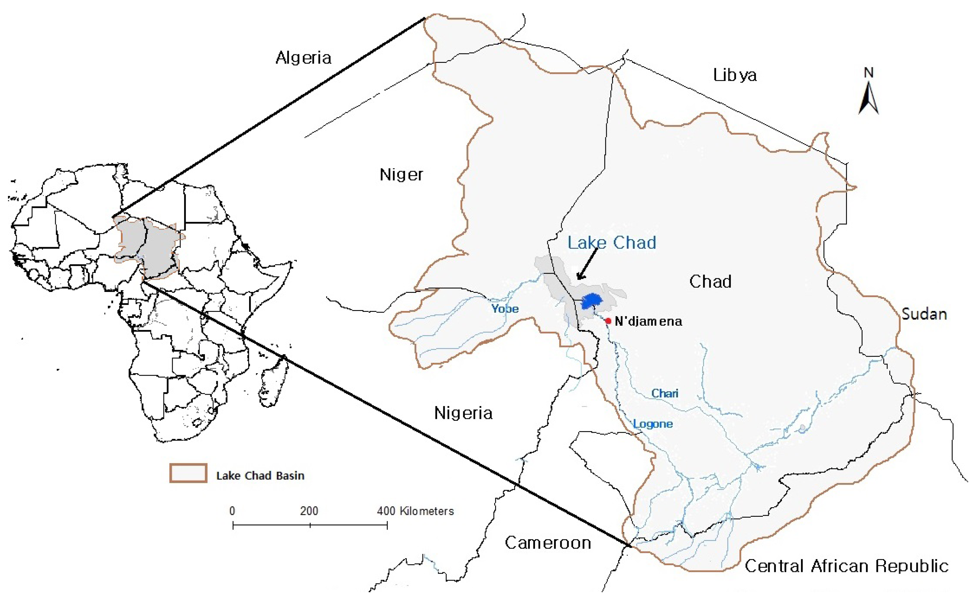
| Location | 6° N and 20° N, 7° E and 25° E |
| Catchment area | 2.4 × 10⁶ km2 |
| Conventional Basin | 427,500 km2 |
| Lake area | 1350 km2 |
| Study Area | Data Products | Reference | ||
|---|---|---|---|---|
| Terrestrial Water Storage | Rainfall | Lake Height | ||
| Lake Chad | GRACE 1 | GPCP 2 | – | [5] |
| Lake Chad | – | – | Sat. Alt. 3 | [25] |
| Lake Chad | – | NOAA 4, TRMM 5 | – | [12] |
| East African Great Lake | GRACE, WGHM 6 | GPCP | Sat. Alt. | [25] |
| Lake Victoria, Malawi and Tamganyika | GRACE | GLDAS, TRMM | Sat. Alt. | [26] |
| Okavango catchment | GRACE | TRMM | Sat. Alt. | [27] |
| Congo river basin | GRACE | GLDAS, TRMM | Sat. Alt. | [26] |
| Lake Victoria, Tamganyika and Malawi | GRACE, WGHM | GLDAS, TRMM | Sat. Alt. | [28] |
| Variable | Dataset | Resolution | Period | |
|---|---|---|---|---|
| Spatial Temporal | ||||
| Terrestrial Water Storage | GRACE | 1° × 1° | 1 month | 2003–2013 |
| Lake Height | Sat. Alt. | 1° × 1° | 30 days | 2003–2013 |
| Rainfall | GLDAS | 1° × 1° | 1 month | 2003–2013 |
| Soil moisture | GLDAS | 1° × 1° | 1 month | 2003–2013 |
| Groundwater | WGHM | 0.5° × 0.5° | 1 month | 2003–2009 |
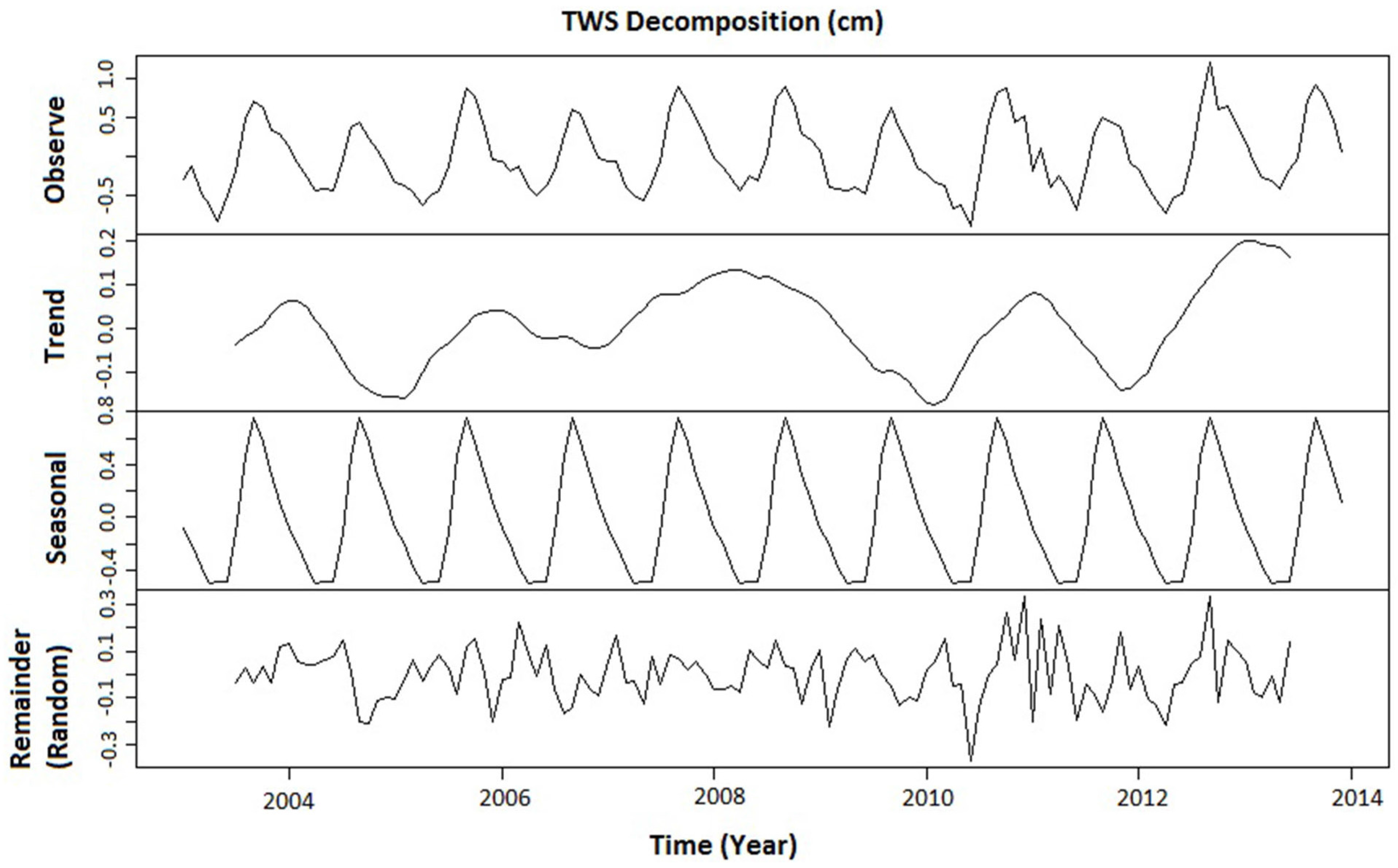
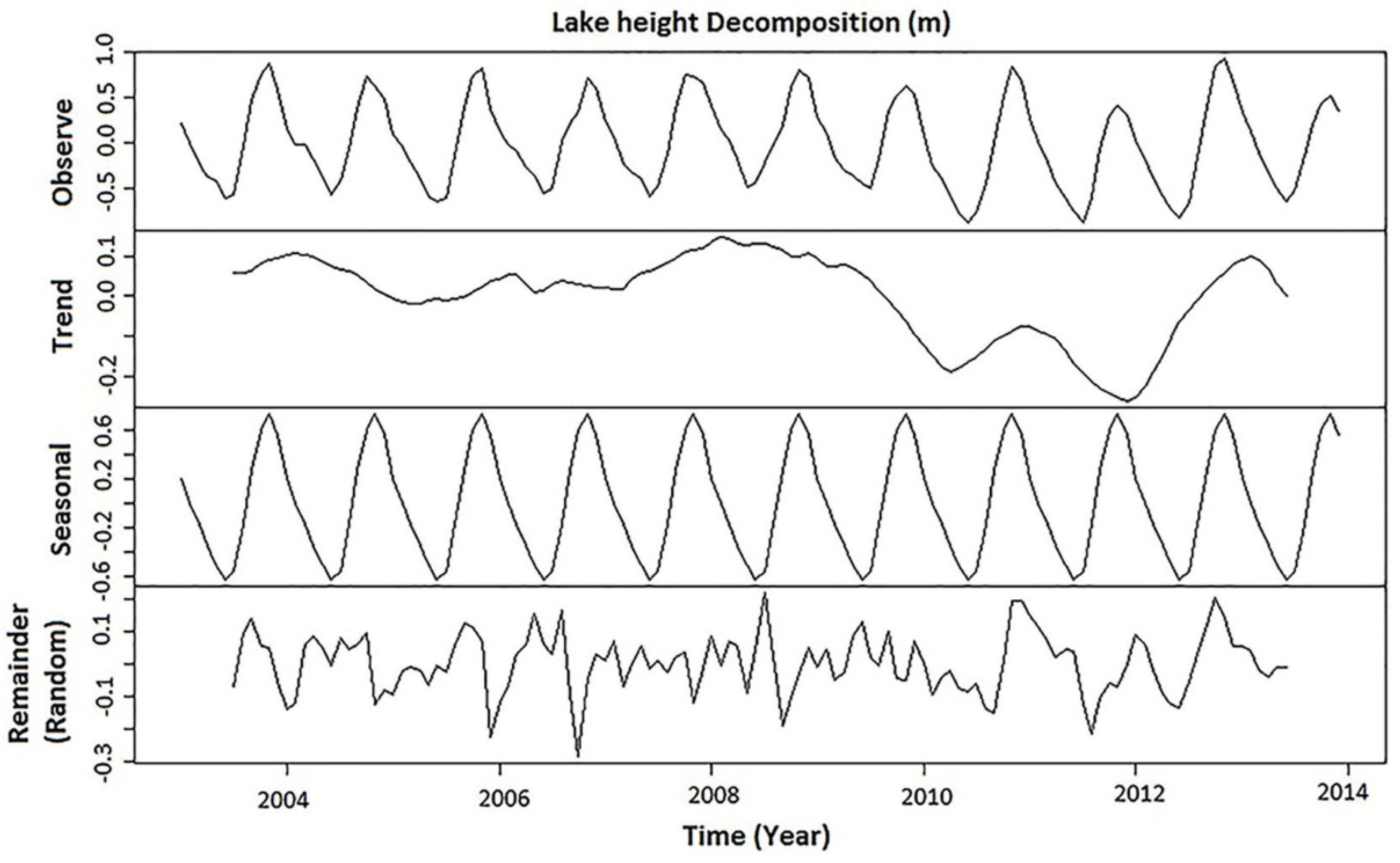
| Period | TWS (cm) | Lake Height (m) |
|---|---|---|
| 2003–2005 | 0.25 | 0.32 |
| 2006–2009 | 0.84 | 0.62 |
| 2010–2013 | 0.38 | −0.78 |
© 2016 by the authors; licensee MDPI, Basel, Switzerland. This article is an open access article distributed under the terms and conditions of the Creative Commons Attribution (CC-BY) license (http://creativecommons.org/licenses/by/4.0/).
Share and Cite
Buma, W.G.; Lee, S.-I.; Seo, J.Y. Hydrological Evaluation of Lake Chad Basin Using Space Borne and Hydrological Model Observations. Water 2016, 8, 205. https://doi.org/10.3390/w8050205
Buma WG, Lee S-I, Seo JY. Hydrological Evaluation of Lake Chad Basin Using Space Borne and Hydrological Model Observations. Water. 2016; 8(5):205. https://doi.org/10.3390/w8050205
Chicago/Turabian StyleBuma, Willibroad Gabila, Sang-Il Lee, and Jae Young Seo. 2016. "Hydrological Evaluation of Lake Chad Basin Using Space Borne and Hydrological Model Observations" Water 8, no. 5: 205. https://doi.org/10.3390/w8050205