Fully Stochastic Distributed Methodology for Multivariate Flood Frequency Analysis

Abstract

An adequate estimation of the extreme behavior of basin response is essential both for designing river structures and for evaluating their risk. The aim of this paper is to develop a new methodology to generate extreme hydrograph series of thousands of years using an event-based model. To this end, a spatial-temporal synthetic rainfall generator (RainSimV3) is combined with a distributed physically-based rainfall–runoff event-based model (RIBS). The use of an event-based model allows simulating longer hydrograph series with less computational and data requirements but need to characterize the initial basis state, which depends on the initial basin moisture distribution. To overcome this problem, this paper proposed a probabilistic calibration–simulation approach, which considers the initial state and the model parameters as random variables characterized by a probability distribution though a Monte Carlo simulation. This approach is compared with two other approaches, the deterministic and the semi-deterministic approaches. Both approaches use a unique initial state. The deterministic approach also uses a unique value of the model parameters while the semi-deterministic approach obtains these values from its probability distribution through a Monte Carlo simulation, considering the basin variability. This methodology has been applied to the Corbès and Générargues basins, in the Southeast of France. The results show that the probabilistic approach offers the best fit. That means that the proposed methodology can be successfully used to characterize the extreme behavior of the basin considering the basin variability and overcoming the basin initial state problem.

1. Introduction

Characterizing the extreme behavior of basin response is necessary for hydraulic infrastructure design, territorial planning, flood management and risk analysis. The magnitude of a flood and its consequences may depend not only on the peak flow but also on the volume, duration and temporal distribution of the hydrograph. Therefore, a multivariate analysis may be needed in some cases. Statistical analyses are traditionally applied in engineering practice to obtain a unique design flood.

The methodologies traditionally applied in engineering practice are statistical analyses with the aim of obtaining a unique design flood. Statistical analyses consist in fitting the most appropriate extreme-value distribution to the observed series of maximum annual discharges, in order to estimate the peak flow associated to a given return period (usually high, e.g., 500 to 10,000 years, in the case of dams). These studies need long and robust observed series to obtain accurate quantile estimates. However, they are usually either not available or not long enough to ensure extrapolations with acceptable uncertainty.

Fortunately, long rainfall series are more often available than discharge ones. This makes it possible to estimate the areal rainfall depth associated to a given return period and to transform it deterministically into a design flood event. However, this approach presents some drawbacks. On the one hand, it erroneously assumes that the return periods associated with the rainfall depth and the derived flood event are the same [1,2,3]. On the other hand, some variables such as the shape and duration of the hyetograph, the initial soil moisture content in the basin or the parameters that characterize the runoff generation processes are arbitrarily defined by the designer. These deterministic assumptions lead to different values of the design flood and hamper the estimation of the real probability of exceedance of the event, as well as its uncertainty.

Some of these drawbacks have been overcome by the derived flood frequency approach proposed by Eagleson [4] that combines a storm event model with a rainfall–runoff (RR) model to obtain the peak flow frequency curve.

Recently, new rainfall and hydrological models have been developed allowing new modifications to the derived flood frequency approach. Some authors have maintained the event-based approach combining a simple stochastic storm generator [5,6] or a more complex model such as the Stochastic Storm Transposition (SST) method [7,8] with semi-distributed [9] or distributed [10] RR models. However, the problem of the characterization of the basin initial state remains unsolved.

This problem can be solved by a continuous simulation approach that combines a stochastic rainfall model such us the Generalized Neyman–Scott Rectangular Pulses (GNSRP) [11,12,13,14,15,16,17,18,19,20] with a continuous RR model. Continuous simulation needs more input data and computation requirements than event-based simulation. In order to simulate long discharge series without an excessive computational cost, most authors have chosen semi-distributed models (ARNO [21]; TOPMODEL [22,23,24,25,26,27]; and HEC-HMS [28]) or lumped models (MISDc [29,30,31,32,33]) or simple and conceptual distributed models (FEST [34] and TETIS [35,36]). A semi-continuous approach has also been developed by replacing observed rainfall events with stochastic ones in a continuous simulation of observed data (SCHADEX [37,38,39]), a Simplified Continuous Rainfall–Runoff Model (SCRRM) which used soil moisture data provided by ground, satellite and reanalysis data [40] and a Hybrid-CE approach which combines a long continuous simulation of the rainfall and a short continuous simulation run as inputs of an event-based rainfall–runoff model [41]. These approaches try to overcome the limitations of event-based models without increasing significantly the computational requirements.

In this context, a new methodology called MODEX is proposed in this study. It combines a spatial-temporal stochastic rainfall generator based on the GNSRP, the RainSim V3, with a spatially distributed, physically-based and event-based RR model, (RIBS) [42,43] through the identification and selection of the annual maximal storm events by the Exponential method and the maximum accumulated rainfall criteria.

The RainSim V3 rainfall model simulates continuous rainfall series that represent the spatial-temporal variability of the observed rainfall keeping its monthly statistics and extreme behavior. The RIBS model is event-based so independent rainfall events have to be identified. The Exponential method is used for this purpose [44,45]. Two consecutive events are independent when they are caused by different weather systems, so the occurrence of the second wet period is not conditional on the first occurrence. This is important from the point of view of flood risk because the consequences of a wet period after another wet period are much worse than after a long dry period. The storm selection reduces the number of simulations and ensures that only the most significant storm events are considered.

Event-based models have some advantages over the continuous models. They could represent better the extreme behavior of peak flows requiring less input data (neither temperature nor evapotranspiration) and the calibration process is simpler due to the smaller number of parameters to calibrate. Furthermore, event-based models require less computation effort so a more complex model, such as a distributed and physically-based one with a higher temporal resolution (hourly or less), can be used. That way the basin spatial variability can be represented; real processes such as infiltration or percolation can be simulated; and complete hydrographs with different shapes and durations can be obtained. These are the main reasons for the selection of RIBS event-based RR model.

The main drawback of event-based models is the initial state characterization, which has a significant influence on the results [46,47,48,49,50,51,52,53]. This paper tries to overcome this problem. Mediero et al. [54] proposed a calibration process for the RIBS model (called here semi-probabilistic), which considers the model parameters as random variables characterized by a probability distribution though a Monte Carlo simulation but using a unique initial state. Based on this process, this paper proposes two other calibration–simulation approaches: the deterministic and the probabilistic (

Table 1. Summary of the three calibration–simulation approaches.

Approach	Model Parameters		Initial State
	Calibration	Simulation	Calibration	Simulation
Deterministic	M Monte Carlo cases	Associated with a 50% probability of exceedance	Random	Related to a intermediate recharge
Semi-probabilistic		Randomized probabilistic values
Probabilistic			Each MC case with all Initial State	Randomized probabilistic values

). The deterministic approach is a simplification of the semi-probabilistic one, which uses a unique value of the model parameters. On the other hand, the probabilistic approach characterizes the initial state and the model parameters through a probability distribution and uses the values obtained through a Monte Carlo simulation. That way the probabilistic approach tries to overcome the initial state characterization problem.

This methodology has been applied to the Corbès and Générargues basins, in the Southeast of France. The results obtained for each calibration–simulation approaches have been compared to show which approach is better. The probabilistic approach offer a really good fit and better than the others, especially when the peak flow is considered. This means the proposed methodology can be used to characterize the extreme behavior of the basin overcoming the main drawbacks of event-based models and also take into account the basin variability.

2. Methodology

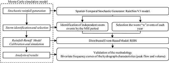
The methodology involves four steps (see Figure 1): (i) stochastic generation of continuous series of rainfall through the RainSim V3 model; (ii) identification and selection of independent storm events from the rainfall series by applying the Exponential method; (iii) rainfall–runoff transformation through the distributed event-based RIBS model, obtaining series of flood hydrographs; and (iv) validation of the methodology and analysis of the results, obtaining a multivariate frequency analysis of the hydrograph characteristics and an uncertainty estimation of the results. These four steps are detailed in the following sections.

2.1. Stochastic Rainfall Generation

Stochastic rainfall models generate arbitrarily long rainfall series that allow characterizing the extreme behavior of the basin and may be used as input in RR models.

The RainSim V3 model simulates the origins of storms based on a uniform Poisson distribution (parameter λ). Each event is composed of a random number of C rainfall cells. Each cell is delayed from the origin of the event according to an exponential distribution with parameter ν and distributed in the space following a Poisson distribution with parameter ρ. Each cell has an independent duration, intensity and radius, which are exponentially distributed (parameters γ, η and ξ, respectively,). The RainSim parameters are summarized in

Table 2. RainSim V3 calibration parameters.

Parameters	Description	Units
λ−1	Mean waiting time between adjacent storm origins	(h)
β−1	Mean waiting time for rain cell origins after storm origin	(h)
η−1	Mean duration of rain cell	(h)
ξ−1	Mean intensity of a rain cell	(mm/h)
γ−1	Mean radius of rain cells	(km)
ρ	Spatial density of rain cell centers	(km−2)
Φ	Vector of scale factors, Φm, one for each rain gauge, m	(-)

. The intensity of rainfall at each point and time step is given by the sum of the intensities of the active cells at such instant.

The RainSim V3 model consists of three modules (analysis, fitting and simulation) and runs in four steps. First, the analysis module calculates the monthly values of a set of statistics which characterize the observed rainfall. Second, the fitting module obtains the value of the model parameters that generate simulated rainfall series whose statistics are the most similar to the calculated from the observed series. The third module simulates synthetic rainfall series based on the adjusted parameters. Lastly, the analysis module is applied again to the synthetic series to compare the statistics from simulated and observed series and check the consistency of simulated ones.

The RainSim V3 model allows the simulation of continuous series of rainfall of N number of years for a set of rain gauges with an arbitrary time step. A detailed description of the model described above may be found in Burton et al. [19].

2.2. Storm Events Identification and Selection

As mentioned above, the selection of an event-based RR model requires the identification of independent storm events by fixing a minimum inter-event period (MIP) between two events (Figure 2). Several methods (such as arbitrary separation, auto-correlation, the exponential method and the range of correlation) have been used to identify individual storms [55,56,57,58].

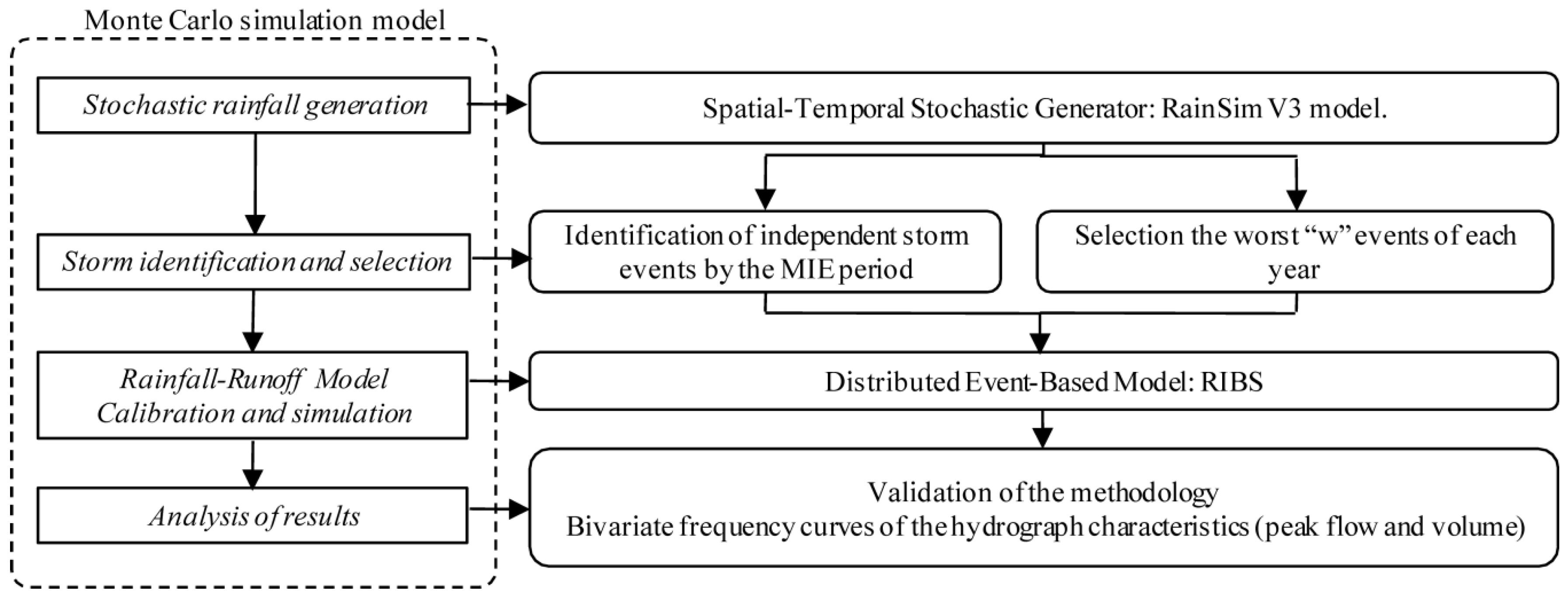
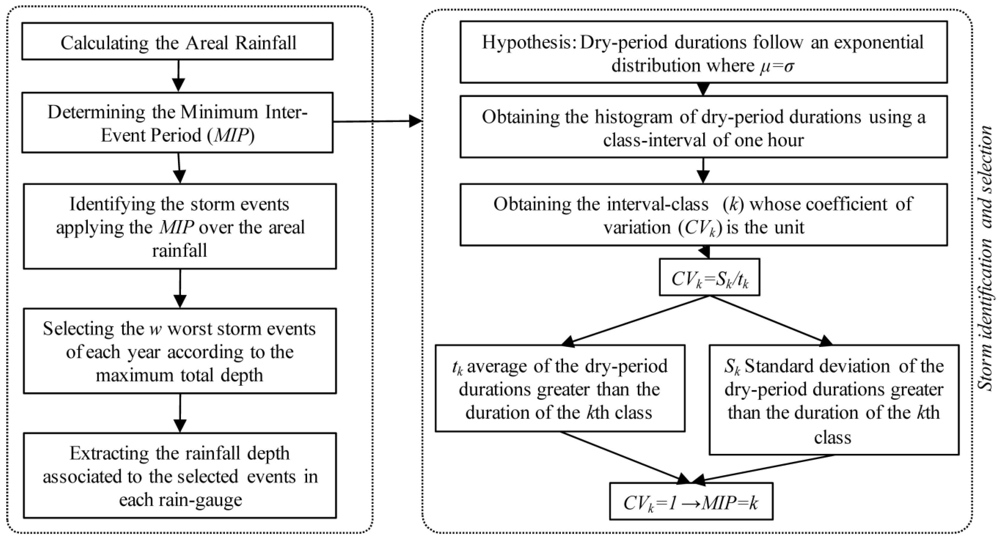
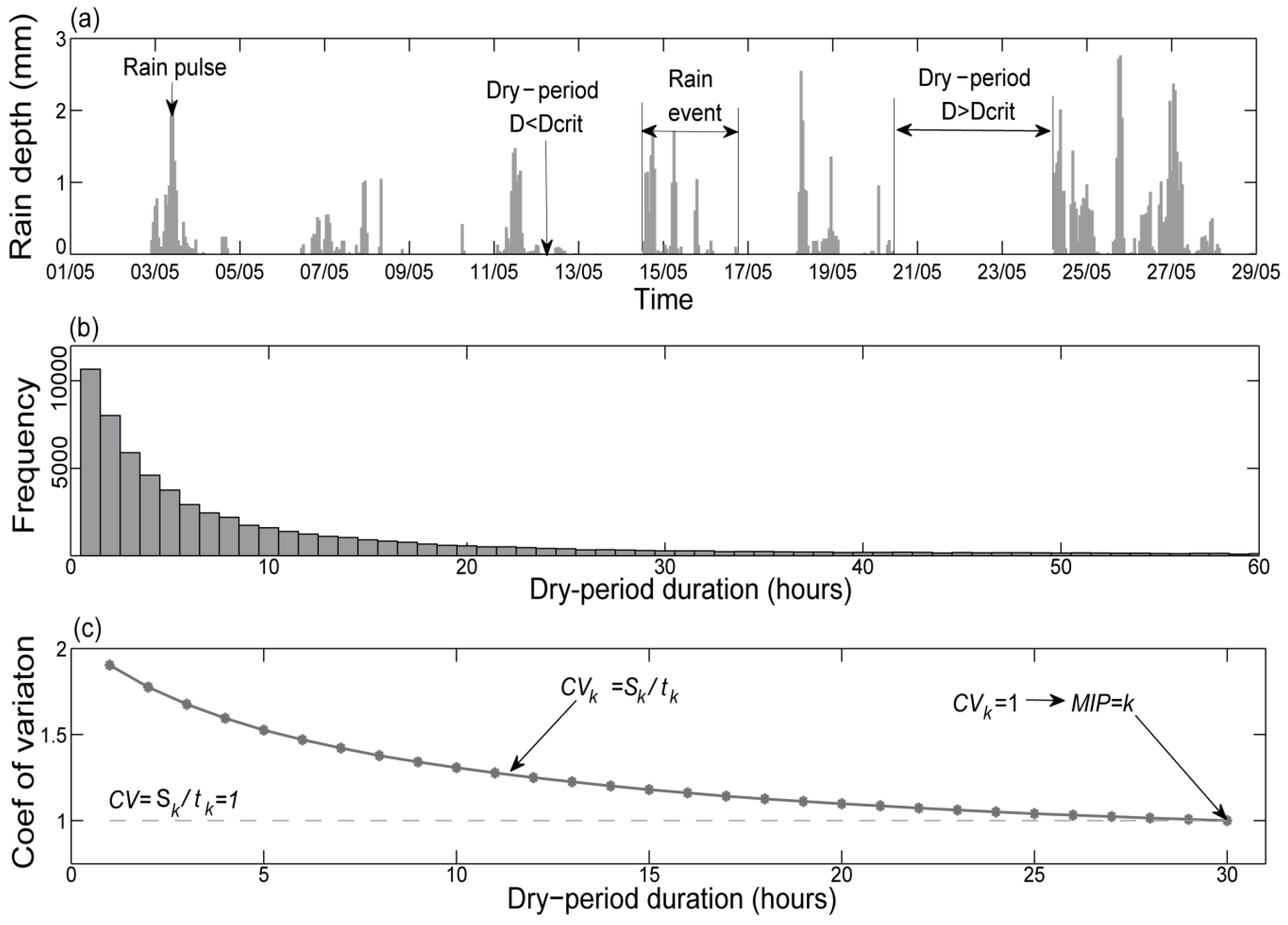
The Exponential method (Figure 3) is used here because it better ensures the independency between events [45]. This method is derived from the Poisson process, which describes the arrival of the storm origins. Consequently, the duration of dry periods can be approximated by an exponential distribution with a mean equal to the standard deviation, $\mu =\sigma$, and therefore with a coefficient of variation, $CV=\sigma /\mu$, equal to the unity. A class-interval width is defined and the histogram of dry period durations is obtained. The CV associated to each class-interval is determined from:

$$C{V}_k=\frac{s_k}{\overline{t_k}}$$

(1)

where k is the number of the histogram class-interval, $s_k$ is the standard deviation of dry period durations greater than the durations of the kth class and $\overline{t_k}$ is its mean. The MIP is the dry period duration at which $CV=1$. A detailed description of the Exponential method may be found in Restrepo-Posada and Eagleson [44].

The exponential method is applied to the basin areal rainfall considering a minimum rainfall threshold of 0.5 mm/h. The storm events that are separated by dry periods equal or longer than the MIP are identified. In order to reduce the number of simulations, a sub-set of w events is selected from each year. As the objective is to characterize the basin extreme behavior, the selection criteria chosen is the maximum accumulated rainfall.

2.3. Rainfall–Runoff Model

The RIBS model simulates the response of the basin to spatially distributed rainfall. It is based on a digital terrain-based model and information provided in raster-style grids that are combined to determine the operating parameters. It consists of two modules: one that involves runoff generation and another of runoff propagation. The runoff generation module represents the soil characteristics by the Brooks-Corey parameterization where the saturated hydraulic conductivity, $K_s$, decreases exponentially in depth, y, in directions parallel, p, and normal, n, to the land surface accordingly to the following expression.

$$K_{S_n}\left(y\right)=K_{0_n}{e}^{-fy}{\left(\frac{\theta -{\theta }_r}{{\theta }_s-{\theta }_r}\right)}^{\epsilon }$$

(2)

$$K_{S_p}\left(y\right)=K_{0_p}{e}^{-fy}{\left(\frac{\theta -{\theta }_r}{{\theta }_s-{\theta }_r}\right)}^{\epsilon }$$

(3)

where ${\mathrm{K}}_{0_{\mathrm{n}}}$ and ${\mathrm{K}}_{0_{\mathrm{p}}}$ (mm/h) represent the saturated hydraulic conductivity in the directions normal and parallel to the surface, respectively, and have to be defined for each soil class; f (mm⁻¹) controls the reduction of the saturated hydraulic conductivity with depth; and θ, θ_r and θ_s represent, the soil moisture, the soil residual moisture and the saturated soil moisture for each soil class, respectively. In addition, ε is the soil porosity index [59]. Surface runoff occurs when either the rainfall intensity exceeds the infiltration capacity or the soil is completely saturated.

The runoff propagation module simulates the runoff routing through hill slopes and river channels. The water velocities in riverbed and hill-slope, v_s and $v_h$ are considered to be uniform throughout the basin for each time t, and are related to each other through the dimensionless parameter $K_v$:

$${\mathrm{K}}_{\mathrm{v}}={\mathrm{v}}_{\mathrm{s}}\left(\mathrm{t}\right)/{\mathrm{v}}_{\mathrm{h}}\left(\mathrm{t}\right)$$

(4)

The riverbed velocity is given by the following equation:

$${\mathrm{v}}_{\mathrm{s}}\left(\mathrm{t}\right)={\mathrm{C}}_{\mathrm{v}}{\left[\mathrm{Q}\left(\mathrm{t}\right)/{\mathrm{Q}}_{\text{ref}}\right]}^{\mathrm{r}}$$

(5)

where $Q\left(t\right)$ is the flow at the basin outlet at time t, $Q_{ref}$ is a reference flow, r is a parameter that accounts for the degree of nonlinearity in the basin, and $C_v$ is a calibration coefficient.

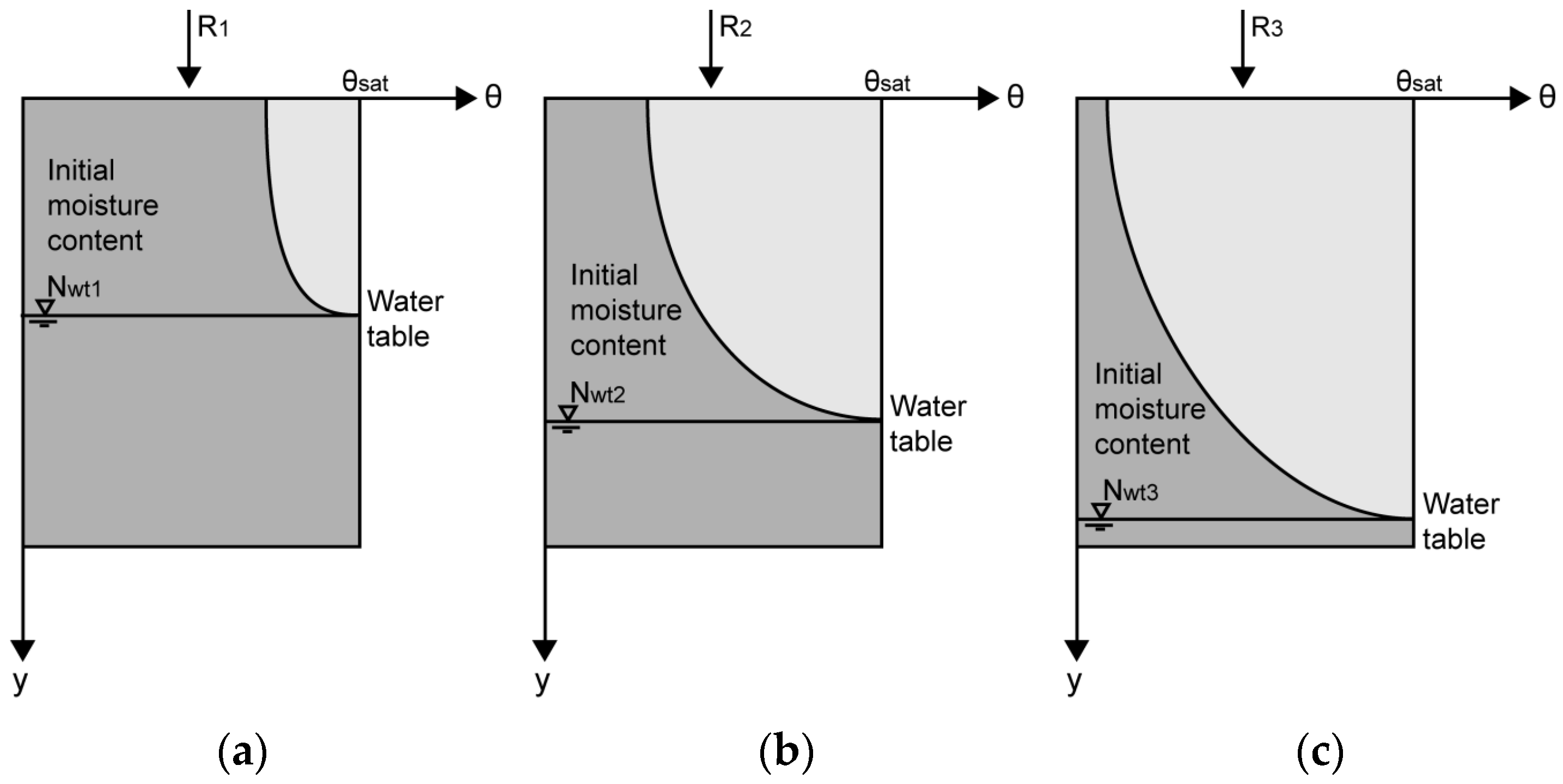
The initial state of the basin is characterized by the water table position in each cell, $N_{wt}\left(x, y\right)$. Initial states are obtained through a groundwater model [60], which considers only water movement in the saturated zone below the water level. This model leads to the balance of the drainage base flows when a long-term recharge, Ri, is applied uniformly to the basin. Larger recharge rates generate higher water table positions and an initial state closer to the soil saturation, $\theta \approx {\theta }_s$, while smaller recharge rates produce lower water table positions and consequently an initial state closer to the dry soil condition, $\theta \approx {\theta }_r$, (see Figure 4). Thus the variable that characterizes the initial state is Ri. A representative set of S initial states are considered, which means an enough large number of Ri values. The recharge values used to generate them cover the whole feasible range. The set of initial states generates a set of hydrographs uniformly distributed between the one obtained with dry soil and that obtained with saturated soil. A detailed description of the RIBS model may be found in Garrote and Bras [42,43].

Calibration and Synthetic Hydrograph Simulation

The sensitivity analysis carried out by Garrote and Bras [42,43] and Mediero et al. [46] concluded that the parameters f, C_v and K_v, have the most influence on the results of the RIBS model. Also the initial state, or Ri that generates it, is determinant for the results.

The calibration process consists on obtaining the parameter values that allow the model representing the best real system behavior by minimizing an objective function that quantifies the error between simulations and observations. However, a given set of parameters that produces good results for one event may generate worse results for another event, because of differences in the catchment response among flood events. A probabilistic approach accounts for this fact and characterizes each model parameter by a probability density function. The model is run with randomized combinations of model parameter values obtained through the probability distributions functions obtained as a result of the calibration process, to account the uncertainties inherent to the model.

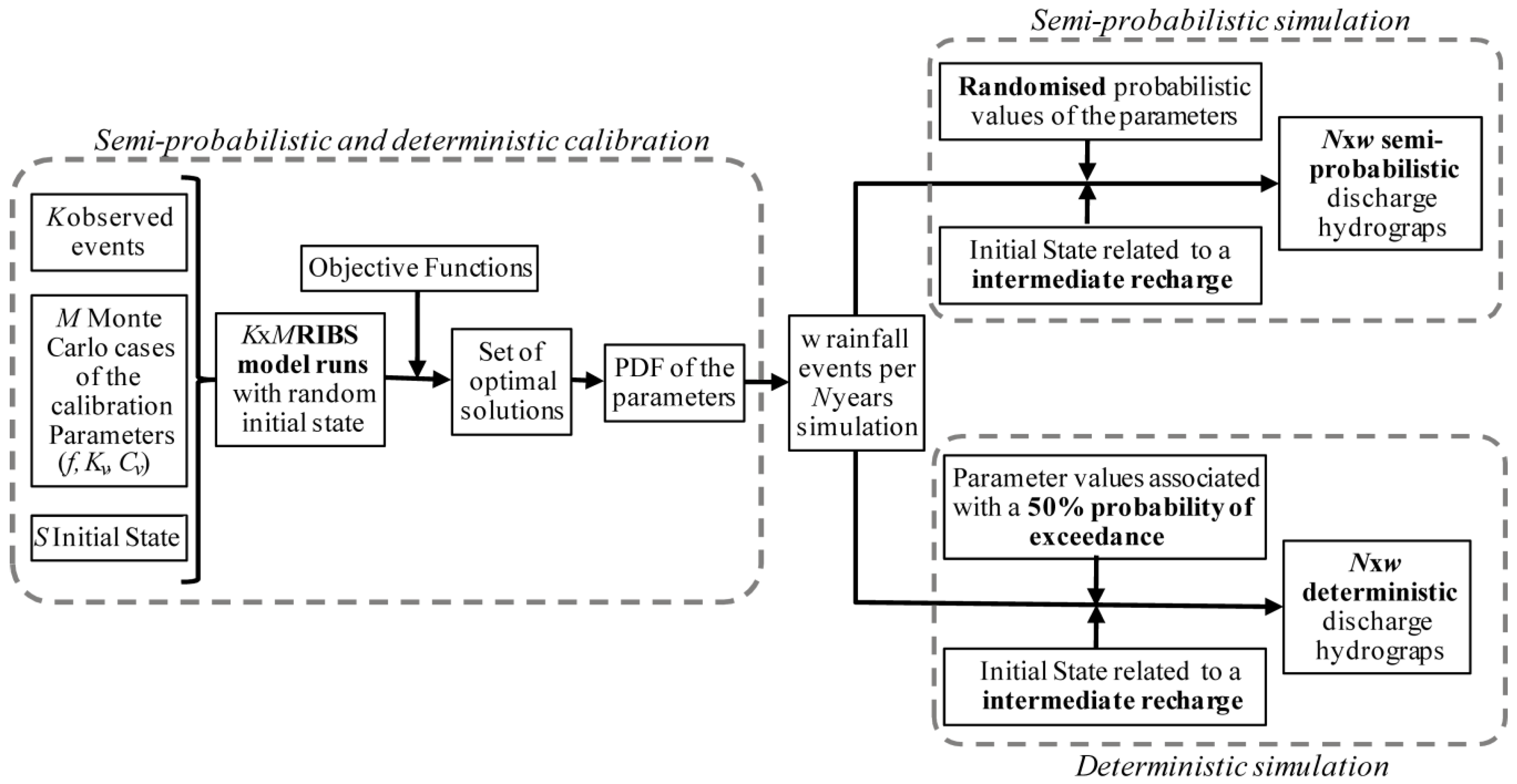
This study seeks to analyze and compare three calibration–simulation processes: deterministic, semi-probabilistic and probabilistic. The process proposed by Mediero [46], called here semi-probabilistic, consists on the simultaneous minimization of a set of objective functions, obtaining a set of optimal parameter value combinations based on the Pareto dominance. Each parameter is characterized by the probability distribution that best represents the set of values obtained as a result.

The choice of the objective functions depends on what aspects of the hydrograph have to be optimized. Given that the proposed methodology is applied to a flood frequency analysis, the objective functions selected represent the peak flow and hydrograph volume:

• Relative error of peak flow (REP), that takes into account the relative difference between the observed ($Q_{max}^{obs}$) and simulated peak flows ($Q_{max}^{sim}$).

  $$REP=\frac{\left|Q_{max}^{sim}-Q_{max}^{obs}\right|}{Q_{max}^{obs}}$$

  (6)
• Volume relative square error (VRSE), that quantifies the relative squared difference between volumes of observed ($V^{obs}$) and simulated hydrographs ($V^{sim}$):

  $$VRSE=\frac{{\left(V^{sim}-V^{obs}\right)}^2}{{V^{obs}}^2}$$

  (7)

The calibration process is applied to K representative observed events. The number of extreme events that have enough rainfall and flow data to be used in the calibration process is usually reduced and cannot be considered representative from a point of view. However, models are usually calibrated with a reduce sample and then validate if the calibrated model reproduce the basin behavior for other events although the reduce number of events used in the calibration process.

A Monte Carlo simulation of M cases is carried out for each observed event, using a uniform distribution of the parameter values (f, C_v and K_v). The range of each parameter values is determined through a previous sensitivity analysis. A random initial state among the S considered is used as input. As a result, the optimal values of each parameter that minimize the two objective functions are obtained (Figure 5).

The optimal values of each parameter are adjusted to several probability distribution functions. The chi-square and Kolmogorov–Smirnov tests are used to select the function that best represents the parameter variability. Finally, a set of synthetic events are simulated by considering randomized probabilistic values of the parameters according to the distributions adjusted and an initial moisture content corresponding to an intermediate recharge (Figure 5).

The deterministic calibration–simulation approach is a simplification of the semi-probabilistic approach. In this case, the calibration process is the same but the synthetic events are simulated with a deterministic value of the parameters which corresponds to an exceedance probability of 50% and the initial state of moisture corresponding to an intermediate recharge (Figure 5).

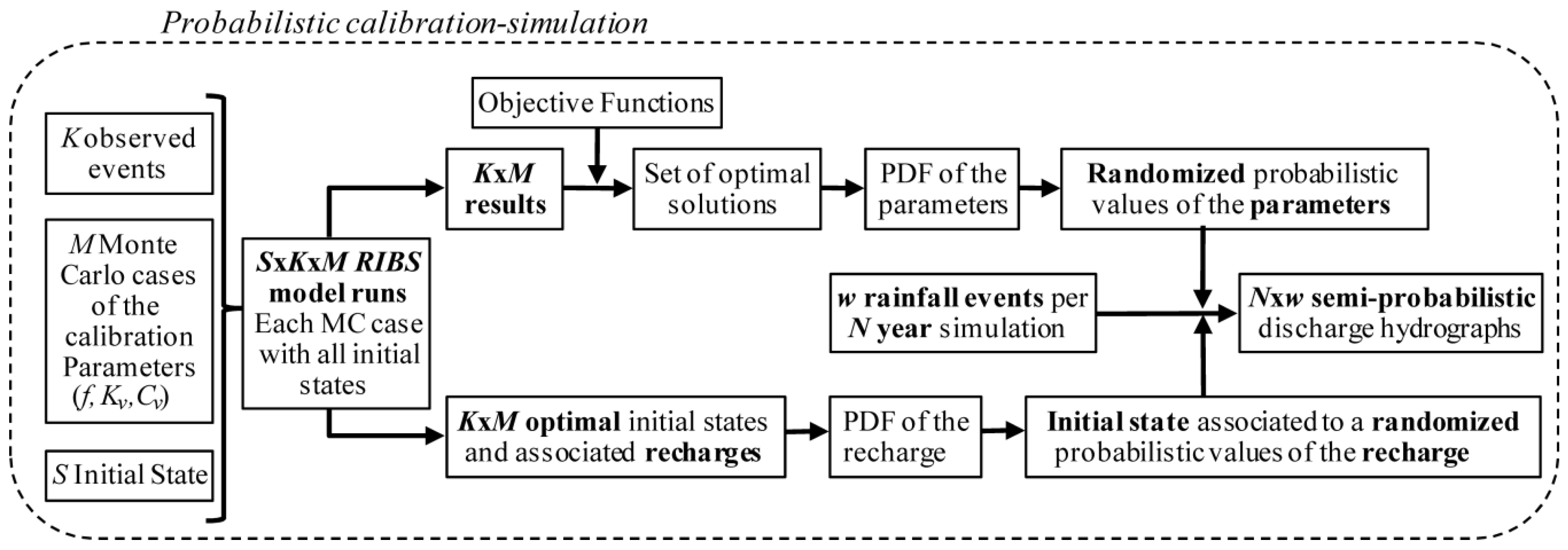
Finally, the probabilistic calibration–simulation approach modifies both the calibration and the simulation processes to characterize the basin initial state by the probability density distribution of the recharge, Ri. Each Monte Carlo case is simulated using all the initial states, selecting the one that leads to a simulated hydrograph with the volume closest to the observed, as the optimal initial state. The set of recharge values associated with the optimal initial states for all Monte Carlo cases and events are adjusted to a nonparametric probability distribution. Then, the multi-objective optimization is applied to all of the Monte Carlo cases simulated with the optimal initial state. The set of Pareto optimal values of the parameters and their probability distributions are obtained. Each synthetic event is simulated with a randomized probabilistic value of the calibration parameters and the initial state associated to a randomized probabilistic value of the recharge (Figure 6).

2.4. Analysis of the Results: Validation

Both, rainfall and RR model results are validated through the comparison between the observed and simulated nonparametric frequency curves. The observed data may also be adjusted to a parametric extreme probability distribution. The Gumbel and Generalised Extreme Value (GEV) distributions are adjusted to the observed data by the L-moments approach, choosing the one which fits best based on the chi-squared test. Due to the length of the observed series, the extrapolation of this function will be representative, approximately, up to a return period of 100 years (Klemeš 2000). Its 95% confidence intervals are also obtained. Therefore, in order to compare the observed series (of only some decades of years) with the simulated series (of thousands of years), P short-series of around 100 years are obtained by random sampling. The median and 95% uncertainty bounds derived from the P short-series are calculated.

The validation consists of comparing the observed, adjusted and median simulated frequency curves, checking if the observed and adjusted ones are contained between the uncertainty bounds. In addition, a quantitative analysis of the goodness-of-fit is performed by means of an objective functions that quantify the error, the Nash–Sutcliffe model efficiency coefficient (NSE). The NSE calculates the relative value of the variance of the residuals in relation to the variance of the observed values. Its optimal value is one.

$$NSE\left(\theta \right)=1-\frac{{\sum }_{Tr=2}^{Tr=100}{\left[x_{Tr}-{x^{\prime }}_{Tr}\left(\theta \right)\right]}^2}{{\sum }_{Tr=2}^{Tr=100}{\left[x_{Tr}-\overline{x}\right]}^2}$$

(8)

where x_Tr represents the value of the adjusted distribution associated with the return period ${\mathrm{T}}_{\mathrm{r}}$, ${\mathrm{x}\prime }_{\text{Tr}}\left(\mathsf{\theta }\right)$ represents the value of the median simulated distribution associated with the return period ${\mathrm{T}}_{\mathrm{r}}$ and $\overline{\mathrm{x}}$ represents the average of the observed values. The interval of return periods considered is between two and 100 years, where the adjusted distribution may be considered representative (Klemeš 2000 [61]).

3. Case Study and Dataset

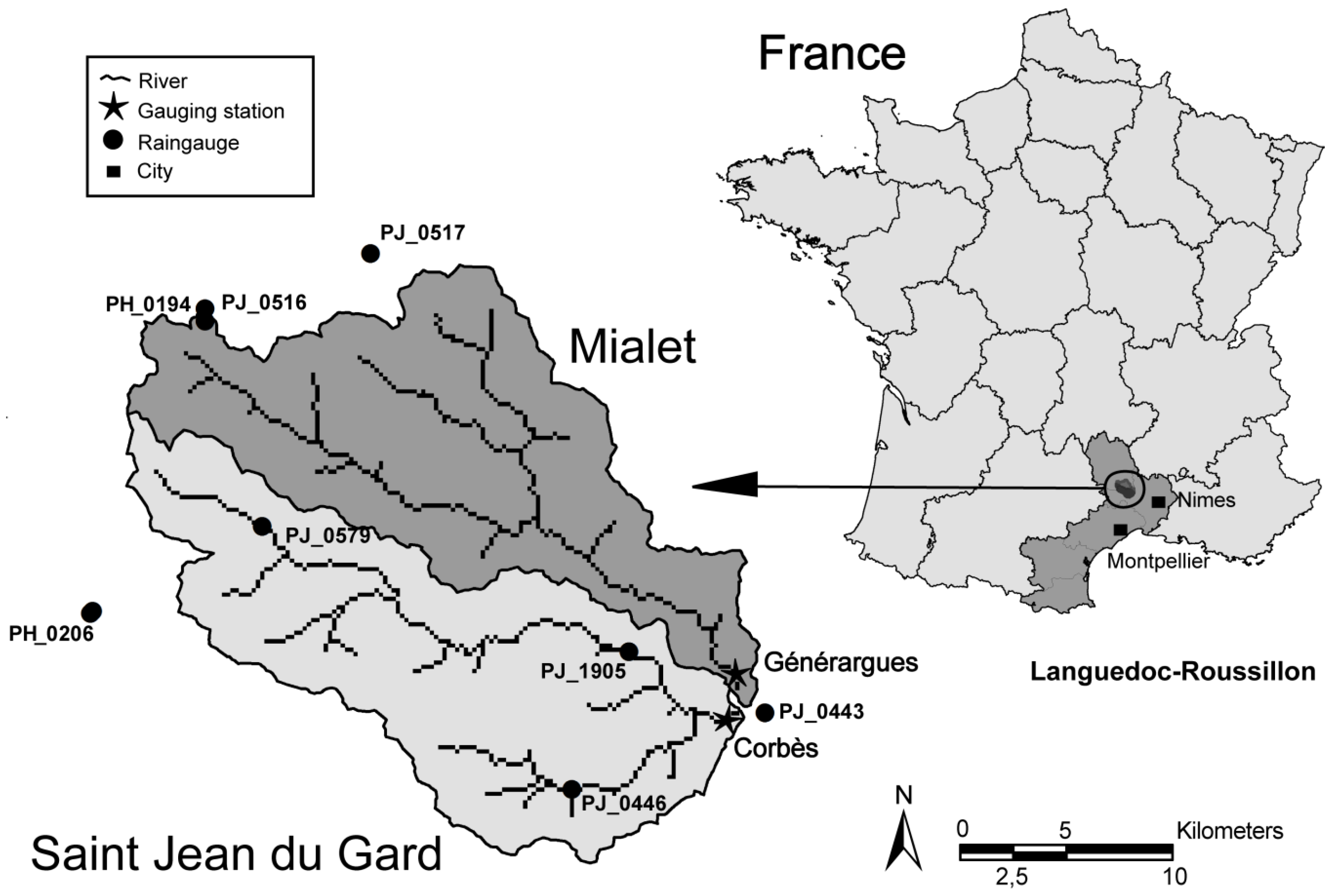
The methodology has been applied to two sub-basins of the Gardons River, Southeastern France: Saint-Jean-du-Gard and Mialet. The Gardons River rises in the Cevennes Mountains and runs through Languedoc-Roussillon, flowing into the Rhône near Beaucaire located between Avignon and Arles. The two sub-basins are located at the headwater of the Gardons River.

The Saint-Jean-du-Gard sub-basin is monitored at the Corbès gauging station and the Mialet sub-basin at the Générargues gauging station. Both gauging stations are located close to the confluence of the two rivers (see Figure 7). The drainage area at Corbès station is 262.3 km², whereas the one at Générargues site is 245.3 km². Both the sub-basins have a typical Mediterranean hydrological regime with major level rises in autumn (in October) and winter (in January), and low levels in summer (in July). A daily rainfall data series of 62 years (1948–2009) is available from eight gauges located in and around the basins (Figure 7) and also from hourly rainfall series (1988–2008) that are available only for two of them (PH_0194 and PH_0206). The flow data are obtained from the two discharge stations that provide hourly and daily data for the period 1971–2010.

From the data series, only 10 representative flood events have enough rainfall and flow data to calibrate the RIBS model (see

Table 3. Flood events used for calibration of the RIBS model.

Event		Maximum Intensity (mm/h)	Peak Flow (m3/s)		Hydrograph Volume (hm3)
			Générargues	Corbès	Générargues	Corbès
1	3 February 1994	15.80	149.00	140.00	13.31	13.75
2	22 September 1994	30.40	438.00	375.00	20.53	19.93
3	2 November 1994	44.00	385.00	372.00	63.94	69.11
4	17 September 1995	19.60	427.00	479.00	16.45	19.97
5	24 November 1995	15.15	262.00	189.00	23.25	25.19
6	11 January 1996	17.82	316.00	359.00	44.24	55.26
7	25 February 1996	8.87	105.00	117.00	14.24	18.10
8	11 January 1998	36.45	317.00	287.00	21.95	27.08
9	19 October 1999	19.24	324.00	290.00	15.18	15.27
10	23 November 2002	26.14	294.00	277.00	20.22	22.46

). Although 10 events cannot be considered representative from this point of view, the model validation results show that the model reproduces quite well the basin behavior.

Drainage areas and slope directions maps, which are necessary for the RIBS model, are obtained from a digital elevation model with 200 × 200 m² cells. Twenty-three soil types are considered based on the Coordination of Information on the Environment Land Cover database [62], obtaining the soil parameters used in the RIBS model according to the Brooks-Corey parameterization.

4. Results and Discussion

4.1. Rainfall Model Calibration

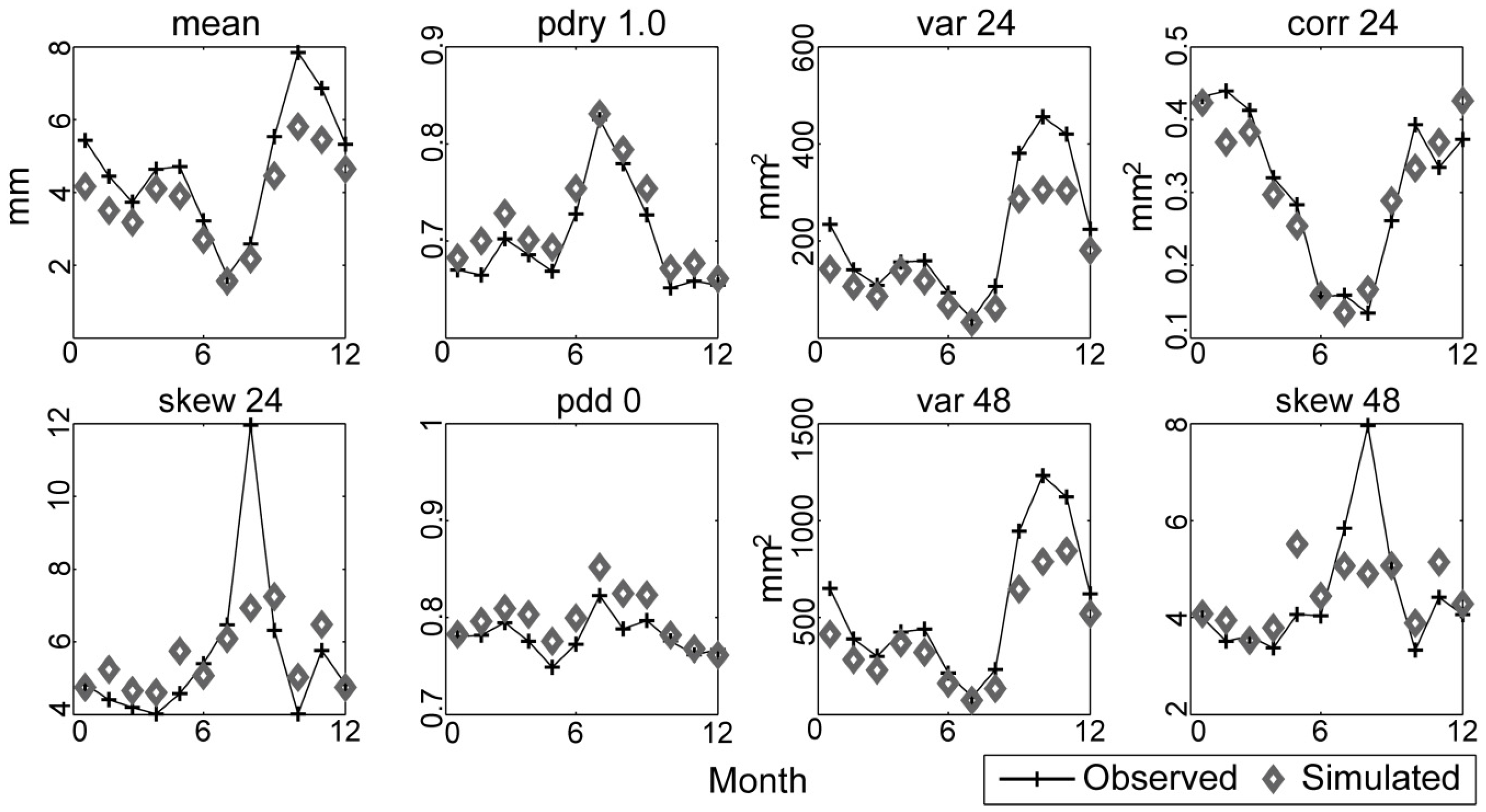
The RainSim V3 model is calibrated from the available observed series for the eight rain gauges. Selected monthly statistics are: the mean 24 h rainfall accumulation (mean); the probability that an 24 h accumulation is less than 1 mm (pdry1.0); the variance of the 24 h accumulation (var24); the correlation of 24 h accumulation of two time series of the same site offset by a lag of 24 h (corr24); the skewness coefficient of 24 h accumulations (skew24); the dry–dry transition probability of 24 h accumulations (pdd0) and the variance; and the skewness coefficient of 48 h accumulation (var48 and skew48). From these statistics, the optimal values of the calibration parameters (λ, β, η, ξ, γ, ρ, and Φ) are obtained.

Based on the optimal parameter values, a continuous series of 1000 years of hourly rainfall is generated. The monthly statistics from the synthetic series are calculated and compared with those of the observed series. The results show a good fit for most of the rain gauges. As an example, the results for the rain gauge PH_0194 are provided in Figure 8.

4.2. Rainfall Model Validation

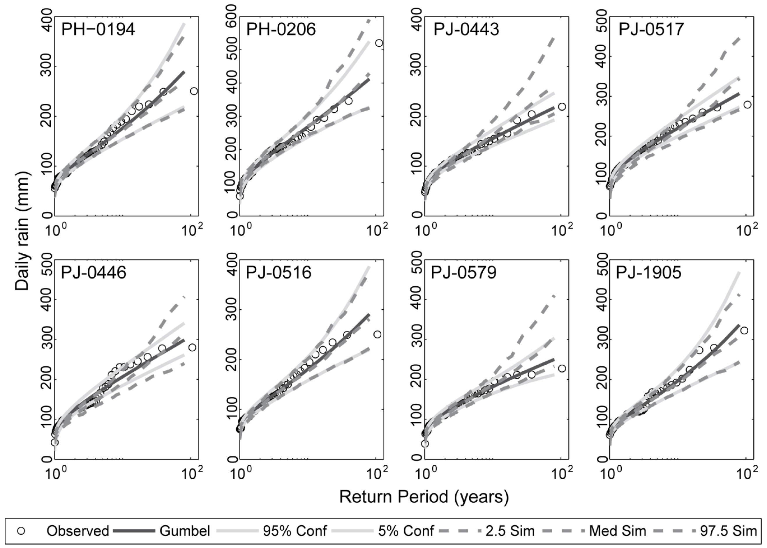
Once the rainfall model is calibrated, a series of hourly rainfall for 6000 years for the eight rain gauges are generated and the series of annual maximum daily rainfall (AMR) are obtained from the observed and simulated rainfall series. Validation of the model is carried out with the series of 62 years of observed AMR and 300 short-series of 125 years sampled from the 6000-year series of simulated AMR by random sampling. The results of the validation are shown in Figure 9 and

Table 4. NSE values calculated for the AMR for the eight rain gauges.

Station	PH_0194	PH_0206	PJ_0443	PJ_0517	PJ_0446	PJ_0516	PJ_0579	PJ_1905
NSE	0.99518	0.99364	0.94334	0.93327	0.9422	0.99498	0.95852	0.99248

.

As it can be seen, the results are very good for all of the rain gauges (see Table 4) with NSE coefficients greater than 0.93.

4.3. RIBS Calibration

The RIBS model is calibrated using the three calibration–simulation processes, considering 10 representative observed events, 1000 Monte Carlo combinations of the calibration parameters (f, $C_v$ and $K_v$) and 25 initial states. The following results are obtained: (a) a probability distribution for each parameter that is common for the deterministic and semi-probabilistic approaches; and (b) a probability distribution for each parameter and for the recharge (initial condition) in the case of the probabilistic approach.

4.4. Synthetic Events Simulation

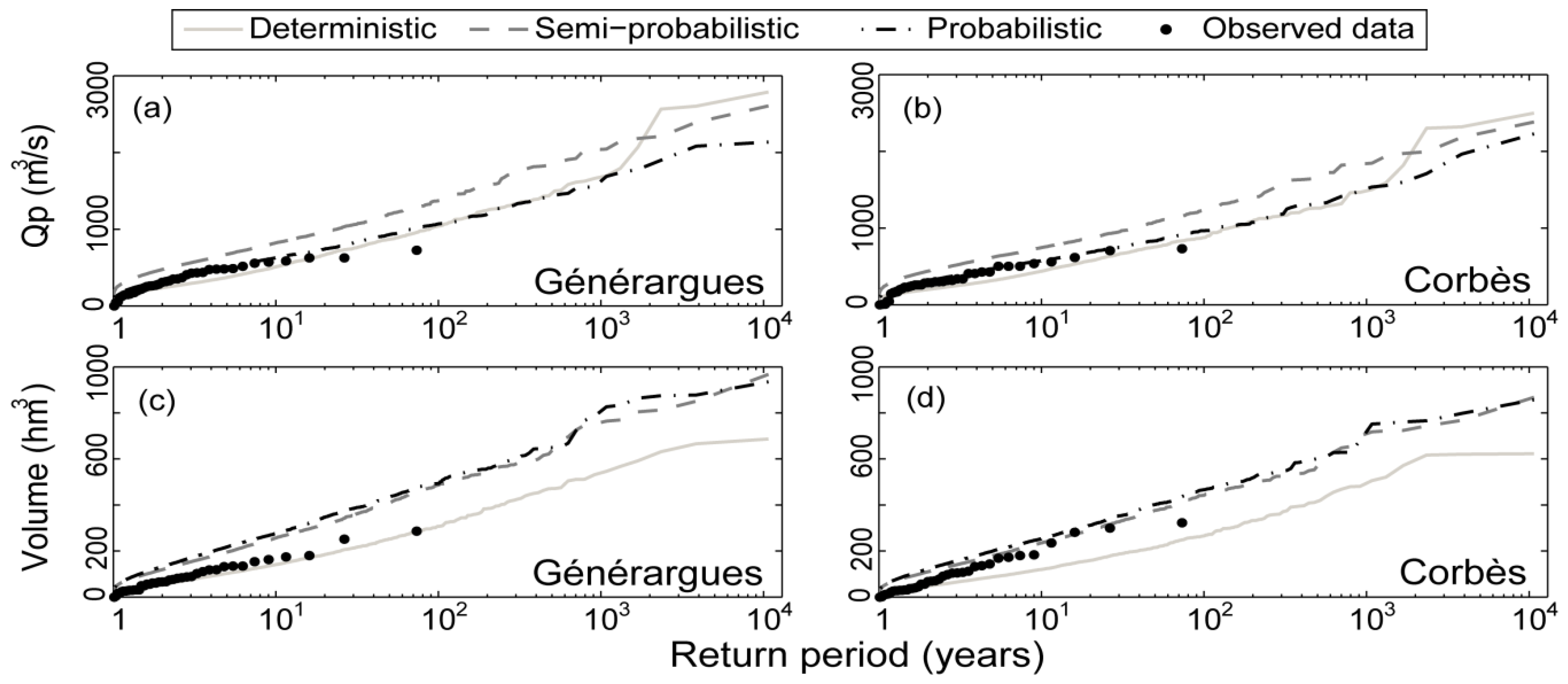
After performing the three calibration–simulation processes, the three series of 6000 years with five events per year were simulated (6000 years × 5 events = 30,000 hydrographs in total), obtaining three series of 30,000 hydrographs: deterministic, semi-probabilistic and probabilistic. These series enable the calculation of the nonparametric frequency curves of annual maximum peak flows and their associated hydrograph volumes (see Figure 10). This calculation is based on the Gringorten plotting position formula [63].

Although the three curves fit the observations sufficiently well for low and medium return periods, the uncertainty increases for the high ones and the simulated curves spread out, with increasing the differences between themselves. In order to determine which type of calibration–simulation process would best represent the behavior of the basin, the validation is carried out.

4.5. Methodology Validation

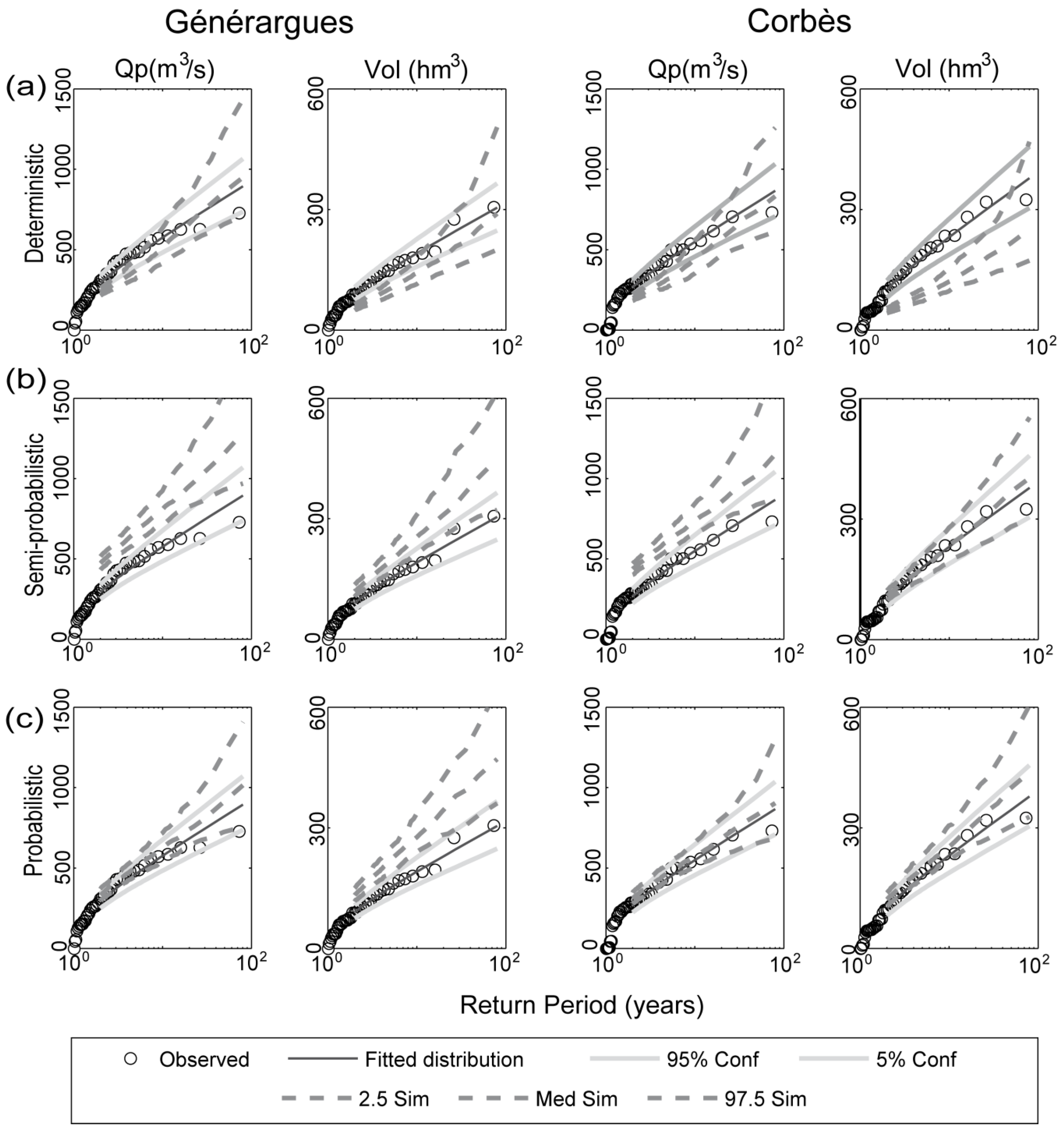
The validation is applied to the 62-year series of observed annual maximum peak flow and hydrograph volume and 300 short-series of 125 years sampled from the three series of 6000 years of maximum annual peak flow and hydrograph volume. The validation results are compared to determine which calibration–simulation approach represents better the basin behavior (Figure 11 and

Table 5. NSE values calculated for the simulated peak flows and hydrograph volumes by the deterministic, semi-probabilistic and probabilistic approaches. The bold text shows the approach that fits best and the italics text shows the worst fit.

Variable	Objective Function	Station	Simulation
			Deterministic	Semi-Probabilistic	Probabilistic
Qmax	NSE	Géneérargues	0.458	−1.764	0.91
		Corbès	0.07	−0.989	0.968
VolQmax	NSE	Géneérargues	−0.195	−0.231	−1.255
		Corbès	−1.598	0.972	0.908

).

The results show that, in the case of peak flows, the probabilistic calibration offers the best fit with NSE coefficients larger than 0.9. The deterministic approach presents an acceptable fit with NSE coefficients smaller than 0.5 while the semi-probabilistic calibration offers a poor fit with NSE coefficients smaller than zero. However, in the case of volumes, the results vary from one basin to another. At Générargues a truly good fit is not achieved by any of the approaches. The cause may be that the considered impervious area by the RR model may be greater than the actual because the RIBS model assumes that the cells through which the river flows are impervious. However, for Corbès, the semi-probabilistic approach leads to the best results (NSE coefficient equal to 0.97), although the probabilistic calibration achieves also a good fit (NSE coefficient equal to 0.91). Therefore, it may be concluded that the best calibration–simulation approach for the cases analyzed is the probabilistic one, which characterizes the initial state and considers the variability of the basin behavior and the uncertainty inherent to the model. In contrast, the other two calibrations do not represent this variability either entirely or partially, which leads to an overestimation or underestimation of the variables that characterize the hydrographs.

4.6. Bivariate and Uncertainty Analysis

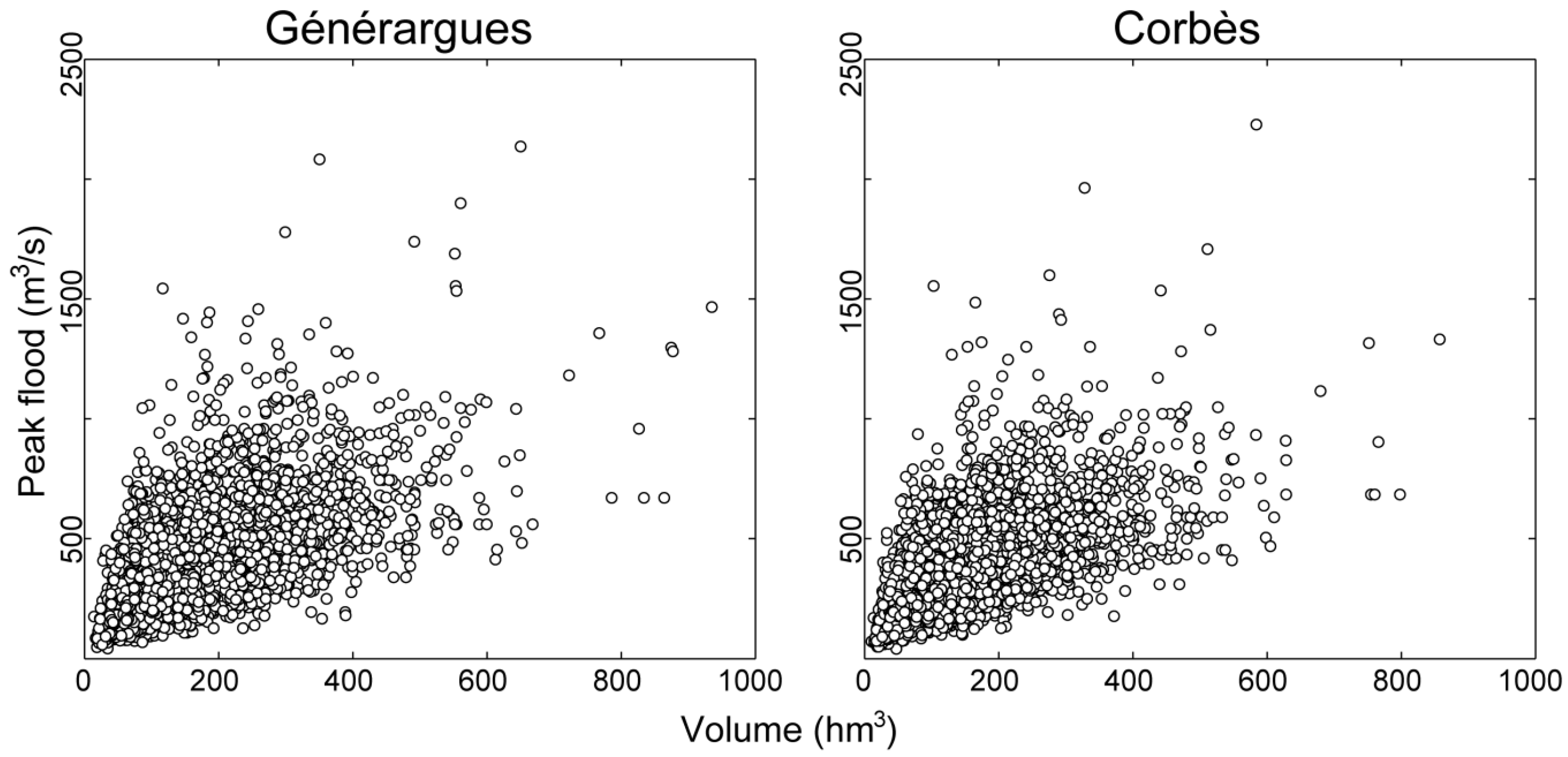
Once the proposed methodology is validated and the probabilistic approach is chosen, a bivariate and uncertainty analysis is carried out. The model results are the series of 6000 years with five complete hydrographs per year that allow characterizing the extreme behavior of the basin. To conduct the bivariate analysis, the peak flows and volumes of the simulated hydrographs are obtained and represented in the flow-volume space (Figure 12). These graphs show that the range of peak flows associated with a hydrograph volume increase with the volume value although the larger the hydrograph volume is, the smaller the number of events is, appearing them more scattered.

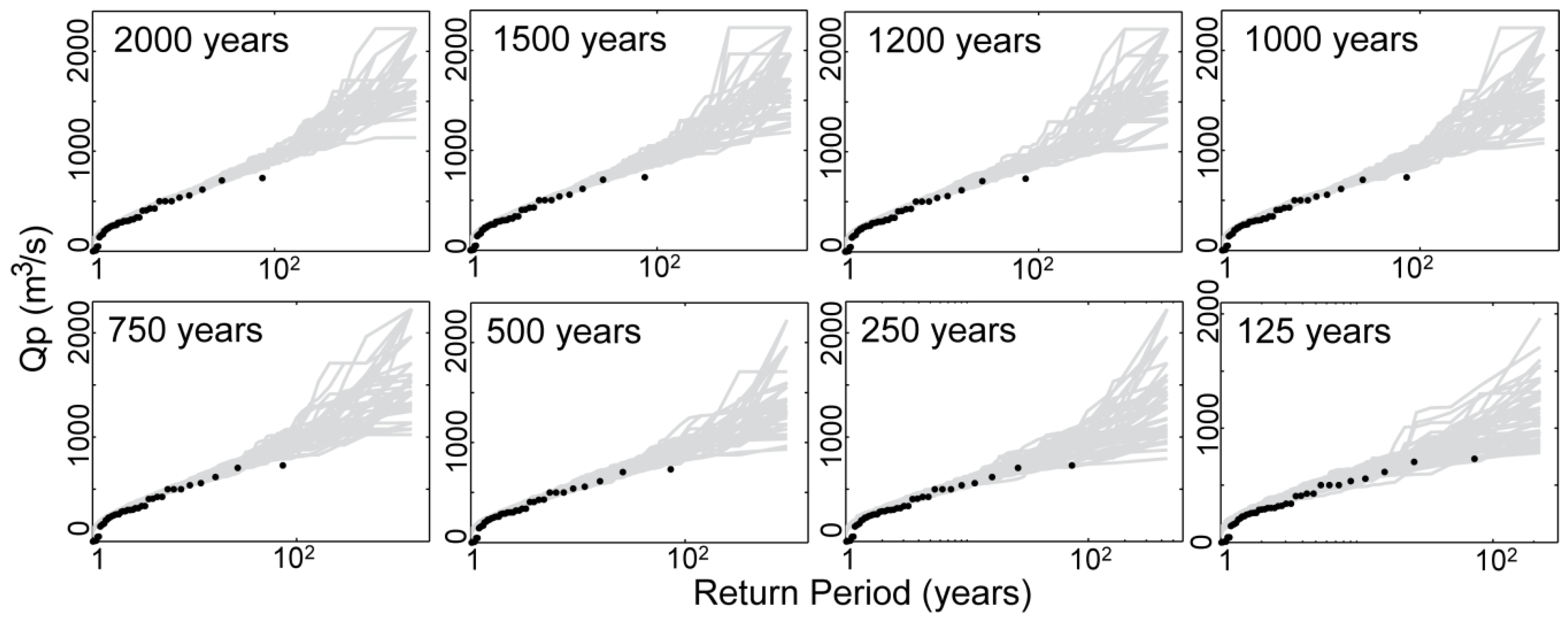
The uncertainty analysis consists on determining the variability in the estimates of the variables associated with a given return period. Hydrograph series of different length (2000, 1500, 1200, 1000, 750, 500, 250 and 125) are obtained from the 6000 years series by random sampling. The nonparametric frequency curves are obtained from each series based on the Gringorten formula and the relationship between the exceedance probability and the return period. Only the uncertainty of the peak flow estimations for the Corbès basin is presented here (see Figure 13).

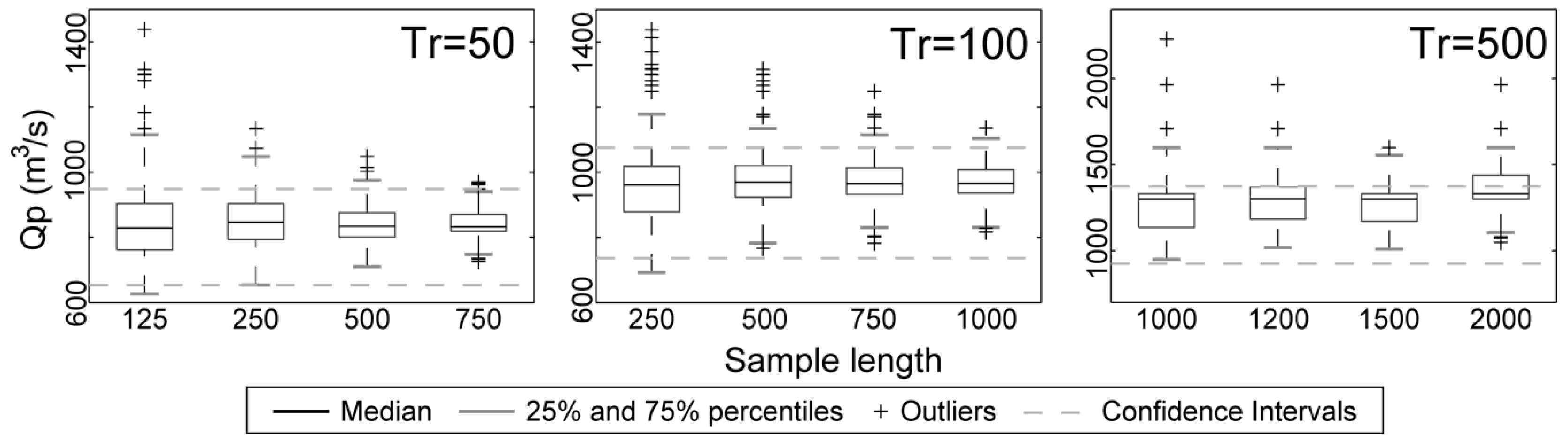
Figure 13 shows that the variability increases with the return period. To see how the variability change with the length series the peak flow values associated with a given return period are calculated from each frequency curve. The different values associated with a given return period and with a series length are statistically analyzed obtaining the 25% percentile (Q1), the 50% percentile (Q2 or median) and the 75% percentile (Q3) quartiles. The results are represented in a box-plot presented in Figure 14. This figure shows that the variability decreases with the length series. Moreover, the median values are bracketed between the confidence intervals, so the results are good enough.

In order to quantify, the uncertainty of the estimations, the interquartile range (IQR) is calculated. The IQR is the difference between the upper and lower quartiles and it is a measure of the statistical dispersion (

Table 6. Values of the first (Q₁), second (Q₂), third (Q₃) quartiles, the interquartile range IQR, and the relative value of the IQR against Q₂ and against the mean of Q₁ and Q₃.

Tr = 500 Years
Data length	Q1	Q2	Q3	IQR	IQR/Q2	IQR/((Q1 + Q3)/2)
1000	1135.0	1300.0	1331.0	196.0	15.1%	15.9%
1250	1183.0	1301.0	1372.0	189.0	14.5%	14.8%
1500	1171.0	1300.0	1331.0	160.0	12.3%	12.8%
2000	1300.0	1331.0	1438.0	138.0	10.4%	10.1%
Tr = 100 years
Data length	Q1	Q2	Q3	IQR	IQR/Q2	IQR/((Q1 + Q3)/2)
250	878.3	961.7	1018.0	139.7	14.5%	14.7%
500	923.0	968.6	1022.0	99.0	10.2%	10.2%
750	932.5	965.0	1013.0	80.5	8.3%	8.3%
1000	936.7	965.4	1008.0	71.3	7.4%	7.3%
Tr = 50 years
Data length	Q1	Q2	Q3	IQR	IQR/Q2	IQR/((Q1 + Q3)/2)
125	761.3	828.8	903.4	142.1	17.1%	17.1%
250	794.1	846.4	903.4	109.4	12.9%	12.9%
500	801.0	833.7	876.2	75.2	9.0%	9.0%
750	819.3	831.8	870.6	51.2	6.2%	6.1%

).

Figure 14 and Table 5 show that the uncertainty decreases with the length of the series and increases with the return period. This means that the longer the simulated series are, the more accurate the estimations associated to high return period are. This estimated uncertainty may be taken into account in the infrastructure design.

5. Conclusions

This study presents a stochastic methodology for the generation of flood event series of arbitrary length by the combination of a stochastic rainfall generator and a distributed rainfall–runoff event-based model through the identification of independent storm events and the selection of a sub-set of events for each year with the criterion of the higher accumulated rainfall.

The combination of the continuous stochastic rainfall generator with the identification of independent events through the exponential method allows an accurate simulation of the rainfall over the basin and the characterization of storm events considering spatial and temporal variability.

The probabilistic calibration–simulation approach proposed here overcomes the main drawback of event-based models, the basin initial state characterization. This approach considers the recharge (initial state of the basin) as a random variable and obtains its probability density function. The results are compared with those obtained for the other approaches (deterministic and semi-probabilistic). The comparison shows that the probabilistic approach better represents the basin behavior than the other two because of the characterization of the initial state, the representation of the runoff generation and propagation processes variability and the uncertainty inherent to the model through a probabilistic calibration and simulation.

The application of this methodology results in a set of complete hydrographs that allows the calculation of the frequency curves of all the variables that characterize the hydrographs and the development of a multivariate analysis.

The main pros and cons of the proposed methodology are:

Pros:

• The application of the RainSim model allows the generation of arbitrarily long hourly rainfall series, even from daily-observed rainfall series.
• The use of a distributed physically-based rainfall–runoff event-based model allows simulating extreme hydrograph series of thousands of years with an hourly resolution.
• The probabilistic approach characterizes the basin initial state and solves the main problem of event-base model.
• This approach also takes into account the basin variability through the runoff generation and propagation.
• The extreme hydrograph series obtained as results can be used in hydraulic infrastructure design, territorial planning, flood management and risk analysis.

Cons:

• The RIBS model assumes that the river cells are impervious, which means that all rain that falls on these cells transforms into runoff. Because of this, the runoff volume produced in the river cells could be greater than the real one and prevent obtaining a good fit.
• To calibrate the RIBS model, it is necessary to dispose of extreme rainfall events and the associated flood events with an hourly resolution. The number of these events is usually reduced, which may difficult the calibration process or make that the results are not quite representative from a statistical point of view
• It should be noted that the study is based on limited case studies and needs more verification in order to validate the proposed methodology

Considering these pros and cons, the methodology is appropriate if there are enough rainfall and flow data to calibrate the models, as well as, if there is a good characterization of the morphological and hydraulic characterization of the catchment available.

Therefore, the methodology presented here may be a useful tool to characterize the hydrological extreme behavior of basins, which, in turn, is essential for the design of hydraulic infrastructures, territorial planning, flood management and risk analysis.