
Large Constructed Wetlands for Phosphorus Control: A Review

Wetland Management Services, 6995 Westbourne Drive, Chelsea, MI 48118, USA
Water 2016, 8(6), 243; https://doi.org/10.3390/w8060243
Submission received: 4 May 2016
/
Revised: 26 May 2016
/
Accepted: 30 May 2016
/
Published: 7 June 2016
(This article belongs to the Special Issue Constructed Wetlands for Water Treatment: New Developments)
Abstract
:This paper reviews aspects of the performance of large (>40 ha) constructed treatment wetlands intended for phosphorus control. Thirty-seven such wetlands have been built and have good data records, with a median size of 754 ha. All are successfully removing phosphorus from a variety of waters. Period of record median concentration reductions were 71%, load reductions 0.77 gP·m−2·year−1, and rate coefficients 12.5 m·year−1. Large wetlands have a narrower performance spectrum than the larger group of all sizes. Some systems display startup trends, ranging to several years, likely resulting from antecedent soil and vegetation conditions. There are internal longitudinal gradients in concentration, which vary with lateral position and flow conditions. Accretion in inlet zones may require attention. Concentrations are reduced to plateau values, in the range of about 10–50 mgP·m−3. Vegetation type has an effect upon performance measures, and its presence facilitates performance. Trends in the performance measures over the history of individual systems display only small changes, with both increases and decreases occurring. Such trends remove little of the variance in behavior. Seasonality is typically weak for steady flow systems, and most variability appears to be stochastic. Stormwater systems display differences between wet and dry season behavior, which appear to be flow-driven. Several models of system performance have been developed, both steady and dynamic.
1. Introduction
In past decades, wastewater treatment plants sometimes discharged to existing marshes. Phosphorus removal was not historically part of pretreatment, and hence considerable P loadings reached those marshes. In other situations, agricultural drainage made its way into neighboring wetlands. For instance, Brillion Marsh in Wisconsin received wastewaters from the town of the same name. A 156 ha natural wetland received incoming wastewater, beginning in 1923. No long-term studies were done, but an intensive study was conducted over the two-year period 1974–1975 [1,2]. The marsh was a uniform stand of Typha latifolia and Typha angustifolia, which received a channel input of treated wastewater. Outflow was also via a channel, and additionally there were small tributary streams to the marsh conveying agricultural runoff. During the two-year study, 16,300 m3·day−1 of influent carried 3.3 ± 2.2 gP·m−3 of phosphorus into the marsh. The hydraulic loading rate of one centimeter per day carried a load of 12.6 gP·m−2·year−1. The outgoing phosphorus was 2.6 gP·m−3, a concentration reduction of 22%, and 2.8 gP·m−2·year−1 was removed by the marsh. This marsh continued to remove phosphorus after fifty years of operation. Similar results were obtained at the 170-ha Cootes Paradise (Glyceria grandis) Marsh near Dundas Ontario, which was found to be removing phosphorus after 60 years of wastewater discharge [3].
Observations at natural wetlands, such as Brillion and Dundas, led to engineered attempts to use natural wetlands for phosphorus reduction. Projects sited in natural wetlands in Michigan and Florida, in the late 1970s, further explored the concept [4,5]. The construction of large wetlands for the purpose of phosphorus control commenced in 1976, with Boney Marsh in Florida [6,7]. Following in 1980 were the Delta Marsh cells in Manitoba [8].
More large constructed P-control wetlands were added in the 1980s, with the development of the Orlando Easterly Wetland (OEW) [9] and Orange County Eastern Service Area Wetland (OCESA) [10], both in 1987. The Balaton system in Hungary began in 1985 [11]. Numerous other small wetlands were constructed during the same time period, many with the expectation of a phosphorus removal benefit. Many other constructed P-control wetlands were added in the 1990s and later.
From these early studies, it was found that constructed treatment wetlands have a demonstrated ability to remove total phosphorus (TP) from various waters, but at relatively low areal efficiencies [12]. Concentration and flow measurements for surface waters entering and leaving the wetland provide the majority of data. A number of mechanisms contribute to the observed P reductions. Particulate forms may settle and become trapped in the litter and floc layers. Dissolved forms may be convected to those bottom regions. P partitions to the soil and sediment surfaces to form storage exchangeable with porewater phosphorus. Biological processes at several scales utilize and convert phosphorus, ranging from microorganisms and algae to macrophytes. New sediments and soils are formed as residuals from the biogeochemical pathways, a process termed bio-accretion. Such new solid accretions are a long-term sink for phosphorus in the wetland. This combination of these physical, chemical and biological mechanisms promotes P removal to new sediments, but generally requires continuously wet conditions for stability.
It is the purpose of this paper to examine and summarize the performance of large constructed free water surface wetlands for phosphorus removal. Herein, “large” is defined as more than 40 ha. The term “constructed” is more ambiguous, but is taken to mean that there are some number of structures and levees that define the wetland. Information from small and natural wetlands is incorporated to some small extent, when useful. The emphasis is on total phosphorus, and upon performance measures, rather than on mechanisms or processes.
2. Performance Measures
There are several different metrics that may be used to evaluate performance. The main goal of the systems under consideration here is the reduction of TP concentrations. Simple measures include:
- Concentration reduction percentage. For large constructed P-control wetlands, it is always the case that, on average, lesser TP concentrations depart from the wetland than enter it. An increase in percent TP concentration reduction would be viewed as an improvement, while a decrease would be interpreted as degradation of performance. This measure does not reflect the flow rate the wetland receives, or the magnitude of the TP concentrations.
- Areal P load reduction. Depending upon many factors, differing P load removals may be achieved. Whatever the level that prevails, long-term trends in the mass of P removed per hectare of treatment wetland are a sign of improvement or degradation as the case may be. This measure reflects the inlet TP concentration and the inlet flow that the wetland receives, but does not distinguish between them.
- Steady-state removal rate coefficients. Simple first-order TP-removal models utilize annual average removal rate coefficients. These vary from system to system, and from year to year. These (partially) compensate for the inlet TP concentrations and hydraulic loadings.
2.1. Wetland Definition
Wetlands have been constructed with a number of cells, arranged in series and parallel. Performance measures may be applied to individual cells, or to combinations of cells, provided that appropriate data are collected. In this overview, an individual wetland is considered to comprise all cells in series in an independent flow path. Parallel flow paths that are structurally independent are considered to be separate wetlands, even though they may be adjacent to one another, and receive the same input water.
2.2. Defining Equations
The design of a wetland system may be for either concentration reduction or for mass removal, but these goals conflict. Interestingly, this distinction has not been well elucidated for P-removal wetlands, but has been described repeatedly for N-removal wetlands [12,13,14]. All large P-removal wetlands have been designed for concentration reduction. Wetland P-removal performance has been documented to follow a first-order rule, according to which P removal is greater at higher P concentrations. This model (Equation (1)) assumes a near-direct proportionality: doubling the concentration above background doubles the removal rate. For a wetland without significant water gains or losses, a simple extension is the PkC* model [15]. Large constructed P-control wetlands typically fit this description to a reasonable approximation [15].
where Ci: inlet TP concentration, gP·m−3; Co: outlet TP concentration, gP·m−3; C*: background concentration, gP·m−3; h: water depth, m; k: apparent rate coefficient, m·year−1; q: inlet hydraulic loading, m·year−1 (=cm·day−1·3.65); and N: number of tanks in series (TIS). It is important to note that the first-order model is imperfect, and rate coefficients may display a dependence on hydraulic loading [16].
TP concentrations decrease as water passes through the treatment wetland, and removal rates also decrease. However, the actual mass of phosphorus that is removed increases with increasing hydraulic loading. Thus, increasing hydraulic loads results in more tons removed, but at the expense of a lesser concentration reduction. This trade-off between concentration reduction efficiency and load reduction may be quantified for the situation of no significant water gains or losses:
where CR: fractional P concentration reduction; PLR: P load reduction, gP·m−2·year−1; qi: inlet hydraulic loading, m·year−1; and qo: outlet hydraulic loading, m·year−1.
The concentration reductions increase with decreasing hydraulic loading (increasing detention time), but not quite in an exponential manner, due to the PkC* model. The maximum load of phosphorus that can be removed results from a hydraulic load so high that little or no concentration reduction is achieved. It is, thus, apparent that there is no such thing as a “typical” or “average” load reduction, because the effects of hydraulic loading and inlet TP concentration create a full spectrum of potential load reductions.
3. Constructed P-Control Wetlands Inventory
The size spectrum of constructed wetlands may be separated into three major groups: mesocosms, small, and large systems. Size matters, because of issues of scale-up. Microcosms and mesocosms are useful for investigating component processes, and, in general, are easily replicated to bolster statistical confidence. But, mesocosms have edge effects, may not have representative vegetation densities, and are not exposed to a realistic set of meteorological conditions. They may contain only a few of the components of a large system, such as soil without plants, litter, or animals. The plants, algae, and microbes in a mesocosm ecosystem are exposed to a time-changing water chemistry, which is different from the spatially distributed patterns of these along the flow direction [17]. Thus, there is a possibility that mesocosm studies produce replicated, well-controlled results of artifacts, rather than processes that actually occur in the field [18,19,20]. Therefore, the database summarized here excludes studies of systems smaller than pilot-scale, generally defined as systems of several tens of square meters extent, located in the out-of-doors.
3.1. Large Systems
There are 94 treatment wetlands of 40 ha or more that were found in the published literature or on the Internet, with a median size of 167 ha. Of these 94 wetlands, 66 are constructed wetlands, with a median size of 210 ha. The remaining 28 are natural wetlands that have been or are being used for water quality improvement, and 20 of these natural systems are forested.
Most of the large constructed wetlands target the reduction of phosphorus (P), and these number 43 of the 66 (Table 1). Some are in a startup condition, and some have only limited amounts of operating data. There are 37 wetlands with extensive phosphorus data, including two that were not specifically intended to remove phosphorus (Columbia and Lakeland). These 37 wetlands total 27,937 ha, with a median size of 754 ha.
Most P-removal wetlands are intended to reduce low P concentrations to even lower levels. The median inlet total phosphorus (TP) for the 37 P-target systems is 114 mgP·m−3; the median outlet TP is 38 mgP·m−3 (Table 2). This 71% concentration reduction (CR) is achieved at a low median hydraulic loading of 2.55 cm·day−1. The amount of phosphorus stored (phosphorus load removed, PLR) in these systems is low, with a median of 0.77 gP·m−2·year−1.
First-order rate coefficients (k) have a median of 12.5 m·year−1. This is somewhat higher than reported medians of 11.0 m·year−1 ([34], N = 20), and 10.0 m·year−1 ([15], N = 282).
The 37-wetland P-removal dataset under consideration contains information totaling 357 wetland-years, out of a total of 586 wetland-years of operation. The average operating age is 15 years. The median number of cells in a wetland is 2.0. All but three of the 37 are in the state of Florida, although 26 of the 66 total large constructed wetlands are outside Florida. Reasons for this Floridian concentration have been discussed elsewhere (e.g., [35,36]).
Many of the Florida systems are designated as stormwater treatment areas (STAs). Twenty-eight constructed large stormwater wetlands were identified, and 26 of these are in Florida. The remaining 38 constructed large systems receive a relatively steady flow, usually via pumping. Stormwater systems receive water on an episodic basis, as determined by rainfall events. Rainfall runoff is pumped or flows by gravity into these wetlands. As a consequence, flows occur mostly in the wet season, and to a much lesser extent in the dry season. Seventy percent of Florida’s rain occurs June–October.
Some systems receive highly treated municipal wastewater (e.g., OEW, OCESA), and others treat river water that has a high content of such treated effluent (e.g., Shannon, Blue Heron). Only Columbia and Lakeland receive high phosphorus municipal effluent, and their design goals do not include P removal.
3.2. Small Systems
A total of 87 small constructed marsh systems were identified as having reasonable data quality and quantity. This means that subsurface flow systems and natural wetland systems have been excluded. The 87 have a median size of 0.25 ha, but range up to 33 ha. Because most of these are pilot systems they have relatively short operating lives and short periods of data record.
4. Period of Record Results
The performance of large P removal wetlands may be compared to a broader population of small wetlands. Phosphorus removal data for large (>40 ha) wetlands is restricted to a smaller number, 37 of the total of 45 listed in Table 1. However, those 37 have an average period of record (POR) of about fourteen years, and data record periods with an average of ten years. The median size of the 37 large data wetlands is 754 ha. In the analyses that follow in this section, annual averages for the entire data record period are averaged, and performance measures computed (Table 2).
4.1. Concentration Reduction
Of the 282 total wetlands reported by Kadlec and Wallace (2009) [15], 274 (97%) lower the phosphorus concentration. The median reduction is 41%. Of the 37 large wetlands, all lower the P concentration, with a median of 71%. The distribution of concentration reductions is rather narrow for large wetlands, spanning 26%–85% for the 10th–90th percentiles (Figure 1). The better performance of large wetlands is at least partly due to their lower hydraulic loading rates, 2.6 cm·day−1 for large versus 3.4 cm·day−1 for the set of small wetlands.
4.2. Load Reduction
There is a large difference between the P load reductions achieved by large wetlands and that of small wetlands: median 0.75 gP·m−2·year−1 for the former, and 2.96 gP·m−2·year−1 for the latter (Figure 2). This may be partially due to the young age of small systems, during which soils have not been P-saturated and vegetation is still establishing. The distribution of load reductions is rather narrow for large wetlands, spanning 0.24–1.32 gP·m−2·year−1 for the 10th–80th percentiles (Figure 2). The small dataset has a median incoming P loading of 10.4 gP·m−2·year−1, whereas the large systems have a median incoming P loading of 1.22 gP·m−2·year−1. In turn, this is partly due to the global median inlet concentration of 0.870 gP·m−3, versus 0.114 gP·m−3 for the large systems.
4.3. Rate Coefficients
There is not much difference between the P median removal rate coefficients for large wetlands (14.6 m·year−1) and small (12.3 m·year−1) (Figure 3). The distribution of rate coefficients is somewhat narrower for large wetlands, spanning 6.1–28.8 m·year−1 for the 10th–90th percentiles (Figure 3). The narrow distribution may be in part due to the narrower range of inlet concentrations and hydraulic loadings that characterize large wetlands.
5. Water Movement
5.1. Flows
5.1.1. Timing
There is a notable distinction between steady flow and event-flow (stormwater) wetlands. In the latter case, large flows occur for only short periods of time. A two-year example of event-driven inflows for STA1W shows that about two-thirds of the time there was no flow into the system (Figure 4). Therefore, the P contents of the incoming and outgoing water were measured using flow-proportional samplers, which provide a flow-weighted mean concentration.
In contrast, the steady flow systems can be grab sampled for P content. For instance, the Apopka Wetland was sampled weekly [37]. Comparable procedures were followed at other systems.
5.1.2. Distribution
In general, water is brought into the STAs via gated structures and spreader canals. This arrangement is believed to help avoid short circuits at the system inlet. Collection is also into a canal at the downstream end of the flow path, and thence to a control structure or pump. Most of the other P-control wetlands also attempt to provide uniform distribution across the flow direction at the inlet, such as Apopka, OCESA and Shannon (Table 1). However, some large P-control systems, such as OEW, utilize point distribution of water.
5.2. Depths
Constructed wetland water depths and flow rates are controlled by either or both the outlet structure and resistance to flow within the wetland. In small wetlands, depth control is generally via the settings of the outflow structure. In contrast, the depths in large wetlands are determined by vegetation density, topography, and flow rate, not by an outflow structure setting [15,38]. However, at low flow, or no flow, an outlet structure can control the depth of the residual water in a stormwater wetland.
Examples of depth profiles through the course of the year are shown in Figure 5. A steady flow system, the Everglades Nutrient Removal Project (ENRP), also operated at relatively steady depths. In contrast, STA56 flow way 7 received no water in the dry season, resulting in complete dry-out to negative depths (below ground). Such complete dry-out has performance implications, because stored organic sediments can oxidize under dry conditions, releasing stored phosphorus [39]. Emergent wetland plants can, in general, withstand dry conditions, but submerged aquatic vegetation (SAV) cannot. Therefore, SAV wetlands, like STA2 C3, are kept hydrated to preserve the desired vegetative cover (Figure 5). Supplemental water is required for this purpose.
5.3. Internal Patterns
The patterns of water movement through the wetland have a significant influence on the efficiency and extent of phosphorus movement. Many of the important biogeochemical reactions rely on contact time between water being treated and biological components and their associated substrate. Any short-circuiting or dead zones will, therefore, impact treatment efficiency. Non-ideal flow patterns in wetland treatment systems have received considerable attention in the literature [15].
Three types of hydraulic inefficiencies may occur in treatment wetlands: one caused by topographical features, a second due to preferential flow channels caused by vegetative non-uniformity, and a third caused by mixing effects, in both the vertical and transverse directions. Large wetlands are particularly susceptible to these effects. Large size makes land leveling prohibitively expensive, and existing topography may be quite non-uniform. Antecedent land uses may mean that remnant roads and ditches may be included within the footprint of a large system. Vegetation establishment in large systems is most often by natural colonization and growth, because of the expense of planting a large area. Such natural regrowth is not uniform, and reflects factors such as water depth, which in turn depends upon topography. Wind fetches in large systems can be quite large. If there exists open water or SAV, then surface water is driven in the wind direction, with opposing return flows created at other depths.
As a consequence, tracer testing has been utilized to assess non-ideal flow effects in large wetlands [40,41,42,43]. Results are extremely variable, with the tanks-in-series (TIS) characterization ranging from 1 to 9. Poor internal hydraulics corresponded to preferential flow routes, while better performance was found for multiple cells in the flow path. The large wetland TIS determinations bracket the central tendency for smaller wetlands, reported as TIS = 3–4 [15].
5.4. Seepage
It is often not technically feasible to provide impervious liners for large wetlands, although lining was done at the Columbia MO Wetland to protect regional potable water supply. Depending upon the transmissivity of the substrates, vertical flows may occur, either as leakage from or into the wetland. If outward leakage constitutes a potential threat to adjacent properties, then the wetland may be rimmed with a seepage collection canal, which collects seepage and redirects it into the wetland. Seepage collection has been done at several STAs.
6. Phosphorus Speciation
The regulatory measure for treatment wetlands is almost invariably total phosphorus. Total phosphorus in water entering a treatment wetland is comprised of several groups of constituents. The analytical categories of particulate (PP), and dissolved organic (DOP) and soluble reactive (SRP) forms comprise TP. These constituents are also mixtures. Particulate P exists in a spectrum of particle sizes and types. Dissolved organic P is comprised of a suite of organic molecules of varying types and sizes. SRP contains mono- and di-basic phosphates, polyphosphates, and other compounds.
The performances of P-removal constructed wetlands can be quite different, depending upon which forms of phosphorus are sent into them. Further, there are interconversions that occur among the various P species. For instance, SRP may be consumed and converted to PP by algae, and PP may decompose, releasing SRP and DOP.
Wetlands receiving flows dominated by PP have been found to remove P by settling and filtration, which occur at rates that are considerably higher than those for total phosphorus ([30,44,45]). For example, the median annual TP removal rate coefficient for the Apopka, FL systems was 15 m·year−1, while the apparent rate coefficient for PP was 32 m·year−1.
The removed PP is not necessarily inactive, but may release some of the particulate phosphorus, which may appear as soluble phosphorus. If the wetland has a low hydraulic loading, then released soluble P can be taken up by wetland processes. However, if the system receives a high hydraulic loading, then the mechanisms that utilize soluble P may not be able to utilize all of the released P. An example of a low-loaded system is the ENRP, which demonstrated reductions of all forms of P without any large seasonal variation (Figure 6). The Apopka project was loaded at a much higher rate, but at similar concentration levels, and behaved much differently (Figure 7). PP decreased in all months, but Dissolved phosphorus (DP) increased markedly in all months. As a result, TP was reduced in all months, but at much higher percentages in the first six months of the year.
Soluble reactive phosphorus pulses are rapidly consumed in wetlands [46,47]. Juston and DeBusk (2011) [48] measured P species on multiple-point transects over multiple years in STA2 Cell 3. The internal P speciation profile showed that SRP was reduced to the analytical detection limit more quickly than DOP or PP, and that SRP was reduced to lower levels. As a result, SRP exiting the STAs is frequently at the minimum detection level (Table 3).
7. Vegetation
Surprisingly, it is not yet clear whether vegetation type is an important determinant of the performance of large P treatment wetlands. This is in large part because of the difficulty of maintaining any particular species, or any particular vegetative community type, on a large scale. There are no system-wide macrophyte monocultures present in any of the large P treatment wetlands. Intersystem comparisons based on vegetation are compromised by differences in driving variables of flow amounts and timing, inlet concentrations, and climatic variations.
The broad categories of vegetation include emergent aquatic vegetation (EAV), submerged aquatic vegetation (SAV) and algal mats (periphyton). However, floating aquatic vegetation (FAV) has been found to volunteer in patches in some systems, including Eichhornia, Pistia, and Ludwidgia. EAV, typically, is dominated by Typha. SAV is often comprised of Chara, Ceratopyllum, Najas, and Hydrilla.
The vegetation patterns in these large systems are typically quite complex and change with time during operational history. Some changes are spontaneous; others are engendered by management activities. The reader interested in the evolutionary details of species present, and their spatial distribution and abundance should consult the parent literature on the individual systems.
In no case has vegetation been harvested in the large systems, except as it occurs as a management strategy, such the intentional replacement of EAV with SAV.
7.1. Florida Stormwater Systems
Early analyses of the Florida STA projects, including size scales ranging from mesocosms to large field-scale systems, indicated that SAV could provide treatment advantages [49]. Accordingly, the flow paths of the STAs were built or retrofitted to contain significant areal percentages of SAV. Performance data now exist for these constructed wetlands, as well as surveys of vegetation percentages for PORs of several years [50]. A bivariate analysis of that data is shown in Figure 8, which indicates no correlation between the rate coefficient and the fraction of EAV (R2 = 0.0005, N = 125 wetland-years).
7.2. Periphyton Systems
There are two strategies that have been explored to facilitate the growth of periphyton in wetlands that contain only very sparse macrophytes (Periphyton STA = PSTA). One technique is to add a layer of calcareous substrate on top of antecedent peat soils; the second is to remove organic soils down to below layers of calcareous bedrock. There is at present one large treatment wetland (STA34 PSTA), which has been in operation for eight years, implemented via method two (scrapedown). The hypothesis has long been advanced that such systems should be capable of achieving very low outflow P concentrations. Low P has been demonstrated at the mesocosm level [51] and at field scale for very low incoming P concentrations [52]. However, other mesocosm, pilot, and field-scale work was not particularly successful [53].
The 40 ha STA34 PSTA project was established by scraping a thin layer of organic soil from the underlying bedrock. It has achieved an eight-year average outlet P concentration reduction from 19 to 11 mgP·m−3, at a hydraulic loading rate of 4.6 cm·day−1 (Table 2). This corresponds to a low P load reduction, and to rate coefficient (16 m·year−1), about equal to the average for other large-scale wetlands.
7.3. Vegetative Transitions
Constructed wetlands usually begin existence with an antecedent cover crop that is not compatible with the hydrologic regime imposed by the treatment function. Over time, a mix of vegetation will develop, primarily determined by hydropattern and water quality conditions.
Most large P treatment wetlands are not monotypic communities, but rather contain a patchwork of open water, SAV, EAV, and FAV. This may in part be due to the system topography, or to intentionally utilizing successive cells with different bathymetries. Vegetation contributes to treatment, and so the amount contributes to treatment efficacy. Phosphorus removal has been strongly linked to the fractional coverage of different community types ([15,54]). Deeper systems, without macrophytes, display lower removal rate coefficients, in the range of 3–9 m·year−1 [55].
Vegetative transitions can be slow to occur, either due to processes of growth or to species competition. The dynamics of transitions have been documented in several of the South Florida Environmental Reports [50]. The example in Figure 9 shows that several years may be needed to achieve vegetative grow-in. In the South Florida STAs, vegetation management is an ongoing process, designed to maintain community health and coverage and to avoid species replacements regarded as undesirable. In other systems species management has typically not been practiced.
7.4. Management Issues
There are conditions in which vegetation is perceived to require management. For large wetlands, vegetation management can be costly and can interfere with the water quality goals of the system. Some of the problems that have occurred include the following:
- Floating cattail islands. It is not uncommon that Typha forms floating mats [15]. In fact, a contiguous mat with 100% cover is conducive to reasonable P removal [56]. The difficulty arises if the mat is not complete, but consists of “tussocks”, with sizes of a few meters to several hectares. These floating islands can move with the wind and can wreak havoc with bottom sediments and water control structures. Removal was undertaken in STA1W Cell 2.
- Dense surface covers of rooted or floating plants. Some macrophytes have growth habits that can include the formation of thick foliage at the water surface, and to a small extent, above water. Hydrilla verticillata and Panicum repens (torpedo grass) are examples that have influenced operations in large-scale P-removal wetlands. Dense growths smother below-water activity. Several STA cells have experienced this phenomenon and have been treated with herbicides as a cure.
- Deep water damage. A number of wetland plants are susceptible to damage by episodic deep water and/or high water velocities. Brief periods of high inundation can be tolerated, as can periods of dryout of varying intensities. However, prolonged deep water can lead to plant uprooting or fatal oxygen deprivation. An extreme example was the loss of vegetation in STA1E Cell 6, in which vegetation export clogged the outflow and stopped operation [57]. Large stormwater wetlands are particularly susceptible to deep water in their inlet zones, because the hydraulic gradients in large systems are controlled by the vegetation density and not by structure settings. The pulse flows that reach a stormwater wetland can and do occur at rates that are many times the annual average flow and are limited only by the capacity of the inlet pumps (if any) and by flow management strategies.
- Wind damage. The fetches of large wetlands can reach many kilometers, creating conditions for large waves and wind-driven water pileup. In the southeastern USA, primarily in Florida, hurricanes and tropical storms often bring very high winds. Some vegetative communities can withstand these events, including firmly-rooted, sturdy emergents. However, softer less well-rooted plants, including SAV of various kinds, cannot. Instances of severe SAV wind damage have occurred, such as in STA2 Cell 3 due to the 2005 hurricane Wilma [57].
8. Soils
8.1. Floc
Investigators have often observed a flocculent detrital layer, or “floc”, overlaying the soil surface in both natural and constructed wetlands, either unimpacted or impacted by excess phosphorus [58,59]. The bulk density of floc is low, ca. 0.05 g/cm3, and, hence, the thicknesses of the floc layers ranges between a few centimeters up to more than 20 cm.
Large amounts of floc have developed in the STAs. For example, the mean floc depth in 13 STA cells in 2003 was 10.9 ± 5.5 cm, weighing 8.1 ± 5.5 kgDW·m−2. The P content was 6.4 ± 3.8 gP·m−2. These accumulations are very much larger than the sum of all TSS inputs, which were approximately 0.1 kgDW·m−2·year−1. This leads to the conclusion that the STAs, and other P-treatment wetlands, manufacture particulate matter and floc.
Floc materials can quickly respond to nutrient enrichment [60], and thus have the most immediate effect on phosphorus in the water column. Floc is suspendable, via shear forces or bioturbation [61]. However, suspended solids concentrations in the flowing water in the STAs is typically very low, ca. 3 mg/L. Therefore, some researchers have hypothesized that particulate P, in the form of floc, is transported downstream via a spiraling mechanism [60].
8.2. Accretion
The long-term storage of phosphorus is dominated by the formation and accretion of the new soils via the processes of sedimentation and bio-accretion. Wetlands with large incoming sediment loads can contribute to solids buildup in the inlet region via the process of sedimentation. Bio-accretion, created by internal generation processes, is likely to produce one or two centimeters per year of new solids [15] and over a period of many years this may influence the wetland hydraulics. This range of rates will not, in general, threaten vegetation, because root and rhizome development can keep pace on the timescale of years.
Early research on impacted natural wetlands in Florida utilized deposited radioisotope tracers to establish accretion rates [62,63]. A newer technique utilizes change points in soil chemistry along a vertical gradient downward from the soil surface [64]. Applied to the Florida stormwater treatment wetlands, both the vertical soil accretion and the P accretion were determined for the cells in eight of the STA wetlands (Table 4). The P accumulated should correspond to the P removed from the water. The soils data show accumulations about double the removed P, but the variability in both measures is quite high.
Accretion may require maintenance activity after a decade or two of operation. The accretions are likely to be spatially non-uniform, with gradient effects in the flow direction, and patchy development. Sedimentation typically creates a delta effect, and bio-accretion is greater in regions of greater water nutrient content. In turn, this can cause preferential flow path development, due to local channelization of new soils, particularly in the inlet zone. These hydraulic changes may occur without compromising the freeboard of the containment levees. Nevertheless, it is possible that sediment removal will be necessary to restore optimal hydraulics. The only report to date of this maintenance activity is from the Orlando Easterly Wetland, where about 20 cm of sediment was removed from a 59 ha inlet zone of the 481 ha system [29]. In that case, the accumulation was due entirely to bio-accretion, because the incoming water contained no suspended sediment.
9. Variability
9.1. Temporal Variability
9.1.1. System Startup
The basins for a constructed treatment wetlands can start from differing initial conditions soil type, and vegetation type and density. When these new wetlands are exposed to a long hydroperiod, it is obvious that some period of adaptation will ensue, during which soils and vegetation undergo changes. It is expected that the terrestrial basins constructed to contain treatment wetlands do not have the full suite of ecosystem processes that are capable of P removal. Sustainable P removal requires and utilizes the full biogeochemical cycle, with all of the size scales, ranging from macrophytes downward through the microflora and microfauna.
Water quality regulatory requirements do not always allow for startup periods. As an example, a large (41 ha) natural wetland near Orlando released phosphorus for several initial months in 1988–1989, engendering enforcement actions and system termination [34]. Current Floridian stormwater wetland operating permits recognize the possibility that constructed wetlands require a period of development. Two initial periods are considered: (1) attainment of concentration reduction, termed net benefit; and (2) attainment of a relatively stable operating mode, termed stabilization.
Most large-scale P treatment wetlands have not had long startup transients, in part due to the strategy of holding the wetland in a no-flow condition until sorption and grow-in processes have stabilized. The STAs were required to achieve concentration reduction before commencing flow-through.
Antecedent Phosphorus
Wetland P-removal performance may be initially influenced by transition from the past history of the soils and vegetation on the site. The large P-control wetlands are often built on agricultural soils, and may have large antecedent stores of soil P. In turn, that may temporarily result in high concentrations in floodwaters. As an illustration, the adaptation period for the northern flow path of STA1W in Florida lasted about one and a half years. During that time, by regulation, it was held in a no-discharge mode to accommodate the transition (Figure 10) [15]. This wetland clearly contained mobile legacy phosphorus, because it was built on a former agricultural field.
In contrast, prior land uses may have involved low levels of phosphorus. When P-rich floodwater is added, inorganic forms of phosphorus partition to soils and sediments. The process is well understood [65]. This initial sorptive capacity for phosphorus will persist only until the new P-loading establishes a new sorbed P equilibrium [56]. As a case in counterpoint, the Shannon Wetland in Texas [28] displayed no startup pattern, neither an enhancement nor decrement (Figure 11). This 98 ha wetland showed no time trend in rate coefficients over the first five years. Vegetation alterations took place during this period, including sparse plantings.
Thus, the initial period of performance may show P release, or lesser or greater P removal than in the long-term. Some systems have started close to that long-term performance. Antecedent soils and their P loading is an important factor in the initial startup performance of the soils. Short-term uptake or release should be anticipated in the operational strategy, and discounted in forecasts of long-term P removal.
Vegetation Grow-In and Rearrangement
Large wetlands are more expensive to plant with candidate vegetation than smaller systems. The large quantities of propagules needed are not necessarily available. Nonetheless, a few large P wetlands have been at least partially planted, e.g., Orlando Easterly and Shannon.
The growth of the full complement of wetland vegetation requires a supply of nutrients that ultimately resides in the stable, fully developed system biomass, both living and dead. Although this new storage of phosphorus can vary depending on vegetation type and density, it is not trivial compared to typical P loadings to treatment wetlands. As a hypothetical conceptual reference, suppose the marsh develops 1000 gDW·m−2 of above- and belowground biomass, with a P content of 0.2%. The grow-in will then require 2.0 gP·m−2. Supposing that the wetland receives 2.0 gP·m−2·year−1 (e.g., 20 m·year−1 of water at 0.1 gP·m−3), and removes half, it would require two full year’s addition of water to supply this growth requirement.
The establishment of the wetland standing crop of phosphorus is not to be counted as a sustainable P-removal function. Nonetheless, it will be reflected in the input/output mass balance for the wetland during its startup period, if any. This uptake will produce an over-estimate of wetland capacity during startup, and should be discounted in forecasts of long-term P removal.
9.1.2. Seasonal Variation
Three factors are likely candidates for modifying phosphorus uptake over the course of a year: (1) water temperature; (2) vegetation growth patterns; and (3) patterns of water addition. Water temperature may modify microbial processes, which are involved in rapid P uptake and in P release during the decomposition of detritus. Substantial amounts of phosphorus are withdrawn from porewaters and surface waters to support plant and algal growth. Temperate wetlands have a period of plant dormancy occasioned by winter conditions, which differs markedly from warm climate wetlands. Most of the large P-control wetlands are ion-warm climates. These systems may also have periods of relative low vegetative activity, but they do not experience the complete growth stoppage seen in temperate systems. Plankton and periphyton, which depend on light and hence on season, are a variable part of the overall biology, and microbial processes are also known to be important. Stormwater wetlands, such as the South Florida STAs, experience incoming flows and concentrations driven by seasonal patterns of precipitation. Accordingly, it is reasonable to expect temperature or seasonal effects in steady flow systems, but those could be masked by seasonal flow effects in stormwater systems.
Large P wetland performance data were analyzed for potential seasonal effects. Several years’ monthly concentration reduction data were folded into monthly means, and examined for patterns during the course of the year. Three types of behavior were identified.
Steady flow systems showed essentially no seasonal variability in concentration reduction (Figure 12). Temperature effects on rate coefficients (k) are often presumed to follow a modified Arrhenius equation:
where kT: rate coefficient at temperature (T) = T °C, m·year−1; k20: rate coefficient at 20 °C, m·year−1; and q: temperature coefficient. Water temperature in the five Floridian systems typically varies only about 10°C during the course of the year [32], but the Shannon Wetland experiences a 20°C annual variation [28]. Only minimal temperature trends have been found for P removal for emergent marshes in general [15]. For six steady flow large P systems, the median q = 1.012, which implies a 13% increase in k for a 10 °C temperature increase. However, Equation (4) removes only 3% of the variability in k values.
A second seasonal pattern was displayed in the performance of the four Apopka wetlands (Figure 13) [30]. Concentration reductions during the first half of the calendar year were 34% ± 8%; and during the second half of the year were 2% ± 9%. A distinguishing characteristic of these wetlands was that most P removal was particulate P. Dunne et al. (2015) [30] speculate that during the second-half periods, dissolved P was released to the water column, possible from decaying algal and plant biomass.
The STAs display a third type of seasonal variation (Figure 14). STAs show decreased rate coefficients during the winter–spring months, which is also the dry season. Relative rate coefficients during the seven dry months were 39% ± 16% of average and during the remaining five wet months were 185% ± 47% of average. Three operational features characterize the dry season months: lower incoming flows, slightly lower incoming concentrations, and slightly shallower depths in the wetlands.
9.1.3. Stochastic Behavior
A sizeable fraction of the variability in outlet concentrations cannot be ascribed to the major driving forces of flow per unit area and inlet concentration. Among other potential causes are actions of animals and wind, and the status of the vegetative and soil components of the ecosystem. This unascribable variability is deemed to be stochastic.
Steady Flow Systems
The framework for interpreting treatment wetland performance, in general, is comprised of a deterministic component, characterized by appropriate equations, together with a stochastic component, characterized by one or more probability distributions [66]. Performance is typically seasonal, as shown in Figure 15.
Therefore, quantification of stochastic variability requires that the performance be seasonally detrended:
where C: outlet concentration, gP·m−3; Ctrend: trend component of outlet concentration, gP·m−3; and E: stochastic component of outlet concentration, gP·m−3. The random variation is captured via a multiplier on the trend value, given by (Y):
The data from Boney Marsh in Florida provides an illustration of the variability to be expected for mean long-term performance for P removal in large wetlands. This wetland received an average inlet concentration of 0.051 gP·m−3 for 1979–1987, at an average hydraulic loading rate of 2.16 cm·day−1, and produced a mean outlet concentration of 0.019 gP·m−3. Figure 14 shows a considerable scatter band around the mean cyclic trend performance for the monthly means of weekly TP measurements.
The upper percentile points of that distribution are of interest for large steady flow P-control wetlands because of regulatory requirements. For instance, the 90th percentile represents the fractional addition to the monthly trend that may be expected to occur one time out of ten during the period of record. Steady flow systems are often subject to “not to exceed” requirements for monthly effluent values.
Table 5 lists percentiles of the monthly Ψ-distributions for phosphorus for representative large P-removal wetlands. These data indicate that the median of the 95th percentile is an additional 79% above the trend, and that the median of the 90th percentile is an additional 59%. For the larger population of P-removal wetlands of all sizes, these medians are higher [15].
Stormwater Systems
The regulatory criteria for the large STA systems are based upon annual performance, and upon multi-year averages as well. Such criteria are founded on the statistical analysis of the variability of annual average TP in the wetland outlet. The 90th percentile of the distributions of annual outlet concentrations for the STAs is 1.67 times the mean over the POR (N = 236 flow path years).
9.2. Spatial Variability
It is very difficult to view a very large wetland as behaving as a “black box.” The size of large P wetlands invites examination of the internal profiles of P concentrations. Two distinctly different procedures have been followed. If the wetland is compartmentalized, with structures conveying flow from one cell to the next, then those intercell flows can be sampled for TP. If flow rates are also measured, then the TP in the intercell flow can be flow-weighted. If the wetland is not compartmentalized, then a grid of interior points may be sampled for TP and other parameters. Often, a spatially uniform grid is sampled, with cross-flow points representing a specific distance from the inlet. In general, it is not possible to measure the flow rate that may be representative of a given sample point. Flow weighting is not possible.
9.2.1. Compartmentalization
Both the P-load reduction and the rate coefficient depend upon the hydraulic loading, which is the water flow per unit of wetland area. A common, but not universal, feature of large P-removal wetlands is compartmentalization, meaning they contain a number of (relatively) independent sequential cells. In the absence of such compartmentalization, inlet regions are, nonetheless, likely to perform differently from outlet regions. Concentrations, and often flow rates, are measured at the inter-cell connection points. As a consequence of the sequential removal of P through such systems, the inlet cells bear most of the P burden. The inlet cells see the highest P concentrations, and are the recipient of solids deposits originating with the incoming water. Downstream cells see less phosphorus, and accrete solids generated by internal wetland cycling.
The number of cells in the large P-constructed dataset range from one to two dozen, but the median is two (Table 1). When performance is analyzed for cells in series, a decreasing trend is observed from cell to cell along the flow path (e.g., Shannon [28]; Lakeland [34]; ENRP [67]). Cell-wise performance information for the STAs was reported through 2012, at which time intermediate cell data acquisition was terminated [68].
9.2.2. Internal Measurements
If the wetland is evaluated in its entirety, internal trends may be subsume, and whole system trends may not be observed. Time-changing zones can be entirely within the wetland as a whole. In general terms, the zone nearest the inlet may undergo alteration in plant speciation, while zones further downstream may retain their species and performance, and at long distances a background ecosystem will prevail [69].
A case in point is the natural Houghton Lake treatment wetland. Although not compartmentalized, it was analyzed at different size scales. The overall wetland comprises 700 ha, and input–output data were collected at that scale. In the initial few years of the project, which has spanned 39 years to date, attention was focused upon an inlet area of some 20 ha [70,71]. The P removal in this small area declined with time over the initial five years. At the opposite extreme, the “performance” of the entire 700 ha wetland did not change over a 30-year history; that is, there was no change in the effluent P concentration [56]. In recognition of this disparity, monitoring of a 100-ha inlet region commenced in year four of operation. This intermediate-sized zone displayed time trends of decreasing k-values over a period of about five years, but there was no k-value time trend over the ensuing 25 years [56].
9.2.3. Internal Behavior of the STAs
Periodically, many of the STAs have been sampled internally for water quality, on grids that extend both parallel to flow and cross flow ([48,72,73,74]). This information is vitally useful in understanding STA performance.
Transect information can be used to determine rate coefficients. These are snap-shots of performance, linked to the instantaneous flows and concentration at the time of the transect. Therefore, transect rate coefficients must be concatenated over the annual flow distribution to be compared to annual rate coefficients, which are determined from flow-weighted averages of inlet and outlet information. However, transect coefficients allow insights into the P-uptake patterns, as these are related to the instantaneous flow rates.
Areal rate coefficients allow forecasts of the longitudinal variation in P concentrations, as these relate to the hydraulic loading up to that distance (Equation (1)). As one moves downstream from the inlet, the upstream hydraulic loading becomes lower, until at the outlet it becomes the loading for the entire wetland. The kC* model fits transect data quite well; for instance, for twenty transects in STA2C3, the average fit was R2 = 0.89 ± 0.09. These instantaneous transect rate coefficients are strongly dependent on flow rate. When the transect data are flow-weighted, the concentration reductions show the expected pattern of decreases with increasing hydraulic loading rate (Equation (1)) (Figure 16). Furthermore, the monthly rate coefficients, determined from input/output data, cluster at the low end of the loading spectrum, and are consistent with the flow-weighted transect information. The mean transect rate coefficient for the five-year period was 44 m·year−1, while for the same five years, the mean annual system rate coefficient was 38 m·year−1.
The instantaneous transect coefficients change with flow, as do the monthly system I/O coefficients. When flows are high, the coefficients are also high (Figure 17). The instantaneous P-uptake coefficients are very nearly proportional to flow. This behavior is distinctly different from that presumed up till now in STA calculations, which has been a rate coefficient invariant with flow.
There is also spatial variability between parallel transects across the flow direction. As an example, TP was measured on transects on 20 occasions over a span of four years, along five parallel paths in STA2 [74]. The average coefficient of variation perpendicular to flow was 25%. The spatial average concentration, across the width of a wetland, is typically lower than the flow-weighted concentration at that same distance. This is due to the fact that slower speed zones occupy the majority of the wetland width, and so spatial sampling emphasizes slow speeds, with better treatment [75]. The difference between inlet and outlet flow-weighted concentrations and the internal spatial averages for STA2 Cell 3 were about 10 μgP/L near the inlet, and about 4 μgP/L near the outlet.
10. Sustainability and Time Trends
A recurring theme in older wetland literature is that when a wetland receives new inputs of phosphorus it will only remove some portion of the incoming load until the system becomes “saturated” with phosphorus. For instance, Richardson (1985) [70] stated: “Wetlands tested as wastewater filtration systems became phosphorus-saturated in a few years, with the export of excessive quantities of phosphate.” Such early misconceptions ignored the soil building that occurs in treatment wetlands, and were subsequently supplanted by acknowledgement of the sustainable P removal to newly created soils [65]. Based on studies of the storage of P in marshes removing phosphorus in Florida marshes, Craft and Richardson (1993) [63] later recognized that “The efficiency of any wetland to store P on a long-term basis is thus determined by the peat or soil accretion rate…”
Although most wetland science literature now correctly identifies accretion as a principal long-term storage for phosphorus (e.g., [62,63]), there still persists literature that does not directly address the soil-building mechanism as a primary route of phosphorus immobilization. For instance, USEPA (1999) [76] states: “New constructed and natural wetlands are capable of adsorbing phosphorus (P) loadings until the capacity of the soils and new plant growth are saturated.” Mitsch and Gosselink (2000) [77] identify only chemical precipitation, adsorption, and plant uptake as removal mechanisms. Crites et al (2006) [78] state: “Adsorption and precipitation reactions are the major pathways for phosphorus removal…” Interestingly, USEPA (2000) [79] correctly identifies the sustainable mechanism as “accretion and burial.” However, identification of accretion removal does not address the question of whether there may be continuing deterioration of the P-removal mechanisms.
At this point in the history of treatment wetland technology, there now exist some monitoring histories of modestly long duration. Those that pertain to large constructed P-control wetlands are of interest here. Time trends allow confirmation of the long-term sustainability of P removal in these marshes.
10.1. Trends for Steady Flow Wetlands
Time trends for steady flow systems are shown in the top part of Table 6. An example is the Orlando Easterly Wetland (Figure 18). This wetland went into operation in 1988, and underwent a period of vegetative grow-in until 1990, and of reducing inlet TP for another two years. Here, the marsh portion (318 ha) is considered. For the ensuing twelve years, phosphorus loads to the system were fairly stable, with modest interannual variability, until excavation management was undertaken in 2002. That twelve-year POR is considered here. Only slight trends were present in performance, as quantified by linear regression (Table 6). Additionally, these trends account for only a small amount of the variability in the three measures: R2 = 0.032, 0.050, and 0.061 for concentration reduction, P load reduction, and rate coefficient, respectively. Excavation was done because this steady flow system had monthly performance criterion, and monthly excursions were becoming more pronounced (Figure 18).
Data was analyzed for nine large P steady flow treatment wetlands, plus two large natural wetlands. Linear regression was used to establish the time-trend slope of the three performance measures, expressed as percent change per year (Table 6). Median rates of change were 0.2, 2.7, and 2.8% year−1, for CR, k, and PLR, respectively. These median rates of change are all slightly positive. However, the linear trends account for only a very small fraction of the annual variability, with median R2 values of 0.087, 0.014, and 0.0.050 for CR, PLR, and k values, respectively. In other words, the interannual data scatters, and displays almost no trends.
10.2. Trends for Stormwater Wetlands
The south Florida stormwater treatment areas form a well-studied subset (N = 19) of large wetlands designed to remove phosphorus. The systems receive pulses of flow on an intermittent basis. Linear regression was also used to establish the time-trend slope of the three performance measures for the stormwater wetlands (Table 6). Median rates of change were 1.0, −0.2, and −7.6% year−1, for CR, k, and PLR, respectively. The median rate of change for PLR is negative, which may reflect lower incoming P loads and/or persistent startup conditions. Nonetheless, the linear trends account for only a small fraction of the annual variability, with median R2 values of 0.093, 0.074, and 0.113 for CR, k, and PLR values, respectively. In other words, the interannual data scatters, and displays almost no trends for CR and k.
11. Ancillary Benefits
The primary objective of the large P-control wetlands is water quality improvement. Secondary benefits that can accrue in treatment wetlands include (1) vegetative biodiversity; (2) protection and production of fauna; and (3) aesthetic, recreational, commercial, and educational human uses [15]. The first of these is not typical of the large P wetlands, because of perceptions of the desirability, or undesirability, of certain vegetation species for water quality treatment. However, the other two ancillary benefits, animal habitat and recreation, are very important in many of the large P wetlands. The large size of these systems makes them especially important as wildlife habitats, because species richness goes up with size [80]. In turn, wildlife attracts fishermen, bird watchers, and hunters.
11.1. Wildlife Use
Large treatment wetlands are popular with fish, birds, and reptiles. Many thousands of waterfowl frequent the Florida STAs and other P-treatment wetlands, although many are American coots (Fulica americana). These make the systems a stopover on winter migration, but also forage year-round on wetland vegetation. Wading birds are also very prevalent, including uncommon species, such as roseate spoonbills (Platalea ajaja), white pelicans (Pelecanus erythrorhynchos), wood storks (Mycteria americana), and flamingoes (Phoenicopterus ruber). Herons and egrets abound.
Fish occur in large wetlands as well. The southerly location of many of the systems creates conditions conducive to the non-native tilapia (Oreochromis aureus). In general, fishing is not allowed in the Florida STAs.
Alligators (Alligator mississippiensis) have been observed at quite high densities in wetland treatment systems with open water areas and high fish populations. Both the Florida and Texas large P wetlands are home to alligators.
11.2. Wildlife Damage
Nutria (Myocastor coypus) are an invasive species from South America, but they now range across southern and northwestern USA. Nutria feed on a broad range of plants in treatment wetlands, including cattails, grasses, water hyacinth, and duckweed. Nutria cut vegetation to build feeding platforms and nest mounds. They are prolific and achieve damaging population densities unless they are controlled by trapping or shooting Nutria have occurred in problematic numbers in many treatment wetlands, including the East Fork Wetland in Texas. From January through December 2010, almost 13,000 nutria were eliminated from the East Fork Wetland. Another exotic, invasive species, feral hogs (Sus scrofa), also caused limited impacts to the wetland vegetation and levees [25].
American coots (Fulica americana) have caused severe damage to the SAV in Florida STAs, They eat the SAV, causing destruction of the vegetative component of the system.
Black-necked stilts (Himantopus mexicanus), burrowing owls (Athene cunicularia), and snail kites (Rostrhamus sociabilis) have all caused interruptions of the operations of Floridian treatment wetlands [33].
11.3. Human Use
The diversity and abundance of birds in and around wetlands attracts bird watchers, who observe that species lists are longer and counts higher when they include large P-treatment wetlands in their counting areas. All the Florida STAs have public access. For instance, STA34 has two public access points, featuring information kiosks, paved parking, concrete sidewalks, and restrooms for hikers, bicyclers, and bird-watchers. A public dual-lane boat ramp is open seven days a week and offers access to 27 miles of perimeter canals. The STA-3/4 East entrance provides parking and toilet facilities, along with informational signage and access to levee trails. The Audubon Society offers escorted driving trips in the STAs on weekends.
The other large P wetlands, such as the OEW and Shannon Wetlands, also have much public use. Thousands of birds visit the Shannon Wetlands, including several types of egrets, great blue herons, wood storks, white ibises, and American white pelicans. In winter, bird numbers soar, because thousands of migratory birds descend on the area. Gators, deer, and feral hogs also frequent the Shannon Wetlands.
A number of wetland bird species are game species and are hunted. Treatment wetlands frequently provide good waterfowl habitat. In a few cases, these treatment wetlands have been used for duck hunting as a recognized secondary benefit. The stormwater treatment constructed wetlands in Florida are open to duck hunting, and are deemed the best hunting spots in the entire state. Alligator densities in the Florida stormwater treatment constructed wetlands have reached proportions sufficient to allow hunting. On designated weekends in specific areas of the STA, waterfowl and alligator hunts are managed by the Florida Fish and Wildlife Conservation Commission.
12. Models
Almost all models of large wetlands, with one exception, address total phosphorus, a lumped measure. As a result, they do not deal with solids movement, related to particulate phosphorus. Soluble reactive phosphorus is known to behave differently from dissolved organic P and from particulate P. Models do not do a good job of describing the very low P concentrations that occur in some wetlands. Yet, a very large effort has been expended on modeling of large P wetlands, which is briefly summarized here.
12.1. Steady State Models
Early models of P removal in marshes were predicated on steady state, or long-term average conditions. This was a necessity created by the nature of the available databases. Historically, hydraulic conditions were presumed to be either a single well-mixed unit (lakes), or plug flow (rivers, wetlands). Removal was presumed to be a first-order process, with rates varying in proportion to the water concentration ([34,81,82,83]). The calibration parameter is the removal rate coefficient, k. Hydraulic models can account for flow patterns intermediate to plug flow or perfect mixing, through the use of the tanks in series (TIS) model. Several large-scale wetlands have been tracer tested, and produced a central tendency of about N = 4–6 for cells or flow paths of a large wetland (see, for instance, [40,41,42]).
12.1.1. Speciation
Total phosphorus (TP) is, in fact, a mixture comprised of particulate (PP), and dissolved organic (DOP) and soluble reactive (SRP) forms. Each fraction of the lumped TP possesses its own net removal rate coefficient. As the mixture passes through the wetland, its composition changes due to weathering.
As shown in Kadlec (2003) [84], and in Kadlec and Wallace (2009) [15], it is possible to account for speciation in modeling without resorting to multi-species models. In the wetland environment, hydraulics and weathering interact to produce the overall observed reduction in a lumped category of pollutants. Weathering behavior in wetland situations may also be represented by a TIS model, where the hydraulic parameter (N) is relaxed to become a fitting parameter (see Equation (1)).
12.1.2. Including Solid Compartments
The lower bound in Equation (1), labeled C*, is the result of internal recycle processes in the wetland, with small contributions from atmospheric deposition. Model fitting research has typically determined C* levels in the range 10–20 mgP·m−3 [48]. The contribution from atmospheric deposition is estimated at about 2–4 mgP·m−3, based on rainfall TP and dry deposition measurements. The contribution of SAV in STA2C3 has been calibrated at about one-third of the total C* [74]. The submerged aquatic vegetation phosphorus model (SAVPM) is a steady state model patterned after the PkC* model, but additionally containing interacting compartments for biomass, recently accreted sediments, and underlying soils [74]. The model was calibrated and exercised for STA2C3, an SAV wetland.
12.2. Dynamic Models
When the wetland is presented with time-varying flows, there can be large effects of the time sequence of those flows. Proper accounting then requires that system dynamics be considered in modeling. This greatly increases the complexity of calculations. It also brings into consideration the various timescales of wetland processes, including the response times of the water sheet and floc (rapid) and those of the sediments, soils, and biota (slow). The stormwater treatment wetlands manifest the collective effects of these dynamic processes.
As a consequence, spatial and temporal models have been explored for describing P processing in the South Florida STAs [85,86]. These involve two or more compartments and account for spatial effects; they are briefly described here. In general, these models of large wetlands get the hydrology correct, including water depths and stages, without excessive parameterization. They also are all moderately successful in describing the high end of the concentration range, i.e., from a few hundred mgP·m−3 down to 20–25 mgP·m−3, on the timescale of a year. However, none are particularly successful at describing wetland performance at the monthly or faster timescale, or in the low concentration range, i.e., less than about 20 mgP·m−3.
12.2.1. Wetland Water Quality Model (WWQM)
This model was developed to describe phosphorus removal in the STAs [87,88,89]. The WWQM is a dynamic model that uses two spatial dimensions. Hydrodynamics are calculated first, followed by chemical interactions between water and four stationary compartments: periphyton, macrophytes, aerobic sediments, and anaerobic sediments. Chemical species include calcium, iron, carbon, nitrogen, and sulfur. As a consequence, the code solves over 100 equations requiring over 200 coefficients. The attendant computational times were found to be quite large. To date, this model has not been successfully implemented. It was originally calibrated to data from cell 4 of the ENRP. This model is not in general use, and has been supplanted by the LOEM-CW model described below.
12.2.2. Exploratory Dynamic Modeling
Researchers working on various aspects of the STAs developed dynamic models of less complexity as an adjunct to investigating specific ecosystem types. One such was the Process Model for SAV (PMSAV). This model was developed to describe the P-removal processes in wetlands dominated by submerged aquatic vegetation [90,91]. It allows P removal from water by two routes: a biologically mediated pathway and a sedimentation pathway. It also splits storage into a biomass compartment, representing the SAV, and an active sediment compartment. It also utilizes a combination of Monod and first-order processes to interconnect the water column and the biomass components. There are seven adjustable parameters. It can be run easily on a desktop computer, and there are minimal calibration issues. This model was used to conduct screening level computations for the SAV alternative for P removal from Everglades Agricultural Area (EAA) runoff. It has been calibrated to phosphorus and biological data from wetlands at several scales, up to 200 ha, in South Florida. This model is not in general use.
A second study-specific model was the PSTA Forecast Model. This model was developed to describe the P-removal processes in wetlands dominated by periphyton [92]. It utilizes a combination of Monod and first-order processes to interconnect the water column and the biomass components. It can be run easily on a desktop computer, and there are minimal calibration issues. This model was used to conduct screening level computations for the PSTA alternative for P removal from EAA runoff. The model considers hydrologic factors (rain, evaporation), but not hydrodynamic factors. It is not a spatial model, and utilizes a single well-mixed unit. Accordingly, hydraulic efficiencies were very low, and the resulting wetland areas needed for acceptable treatment were very large. At the present time, this model is not in general use.
A third dynamic forecast model was used to explore design and operational strategies for the whole set of STAs, the Everglades Phosphorus and Hydrology (EPH) model. This model spatially discretized an STA into plug-flow cells in series, selected by the user to reflect landscape and water quality regions. It was simplified by consideration of only a few transfers, and by the selection of a monthly time step. Phosphorus removal was calculated using a first-order areal uptake equation, and return i taken to be zero order, and operative only during dry periods [93]. EPH was used to theoretically investigate the results of different operational and design strategies for the STAs. This model is no longer in general use.
12.2.3. The Dynamic Model for Stormwater Treatment Areas (DMSTA)
The STA treatment wetlands operate in a dynamic mode. The principal parts of DMSTA include hydraulics, water TP, and stored P. Storage in solid compartments occurs during periods of high phosphorus availability, and release back to the water occurs in periods of P famine. Permanent removal is to residual sediments containing unavailable P. DMSTA [55,94] is an unsteady state model that removes phosphorus to permanent burial in proportion to the amount of labile P in storage. There is a generic labile pool of phosphorus, in addition to the permanently buried P. That labile pool is presumed to be drawn down by a return flux, or bleed-back. Temporal variations in the water budget (flows, rainfall, evapotranspiration, seepage, storage) are also simulated. DMSTA allows for spatial variability via cells in series or parallel, and accommodates PTIS for each wetland cell.
DMSTA does not attempt to describe the startup of a wetland. For wetlands built on agricultural soils, there is generally a period of startup, during which internal and outlet P concentrations exceed input values. The length of this period is dependent on the size of the antecedent P load contained in the soils. During startup, the wetland undergoes the initial stages of development, such as increases in biomass and the extent of areal coverage. However, the occurrence of a switch to a condition of net P removal does not necessarily signal the end of the ecosystem transition, which may continue over an extended period of stabilization. Data show that startup and stabilization may take two or more years for a newly converted wetland [50]. DMSTA avoids startup by seeking a stationary state solution for repetitive time series.
12.2.4. Transport and Reaction Simulation Engine (TARSE)
This model solves the advection–dispersion equation on an unstructured triangular mesh and incorporates a wide range of user-selectable mechanisms for phosphorus uptake and release parameters [95]. In general, the phosphorus model contains transfers between stores; examples of stores that can be included are soil, water column (solutes), pore water, macrophytes, suspended solids (plankton), and biofilms. Examples of transfers are growth, senescence, settling, and diffusion, described with first-order, second-order, and Monod types of transformations. Local water depths and velocities are determined from an existing two-dimensional, overland-flow hydrologic model, the South Florida Water Management District Regional Simulation Model.
There are nine state variables, including particulate and soluble P in groundwater, porewater, and surface water, together with plants and microbiota [95]. There about 17 transfers of P among compartments, each requiring a rate model and at least one adjustable parameter. Calibration is therefore difficult, and subject to the estimating ability of the user.
The model was applied to one cell 4 of the ENRP [96]. Inflow total phosphorus concentrations and flow rates for the period between 1995 and 2000 were used to simulate cell 4 phosphorus removal. The long-term mean TP at the outlet, 22 mgP·m−3, was matched well, but the root mean square error between model and data over six years was 11 mgP·m−3 for outlet TP. Flows to this cell were relatively steady during this period, and thus the pulse response of the model was not severely stressed. This model has not been used in design, or in the evaluation.
12.2.5. Lake Okeechobee Environment Model for Constructed Wetlands (LOEM-CW)
This dynamic model attempts to describe movement of water, nutrients, and solids in three dimensions [97,98]. The data demands are very high: for example, hourly wind, solar radiation, air temperature, relative humidity, evapotranspiration, and cloud coverage as the external forcings. There is extreme complexity in both the water quality section (130 model parameters) and in the sediment section 27 state variables [99]. As a result, the model requires large amounts of computer execution time. LOEM-CW has been applied to the western flow path of STA34. The root mean square error between model and data over six years was 19 mgP·m−3 for outlet TP, which had an observed mean of 23 mgP·m−3 [98].
13. Economics
The large P-control wetlands are costly to build and operate, because of their size. However, they are not usually planted, nor is a liner typically used, and those two costs comprise about 40% of the total capital cost for smaller surface flow [15]. The large wetlands are not located in areas of excessive land values. As for any treatment works, there is an economy of scale that lowers the per hectare cost [15]. Delivery of water to a large wetland may require very large pumps, which may partially offset an economy of scale.
The median capital cost for 16 large P-control wetlands was $69,000 per hectare, of 53–6742 ha, median 630 ha. In contrast, the median cost for 39 small constructed wetlands, of 1–40 ha, median 6.3 ha, was $132,000 per hectare. These 2016 capital costs do not, in general, include the cost of land acquisition.
The median operation and maintenance (O&M) cost for nine large systems, median 2,210 ha, was $770 per hectare per year. The median operation and maintenance cost for 17 small systems, median 6.0 ha, was $3,620 per hectare per year. These 2016 O&M costs do not, in general, include the cost of water quality monitoring.
14. Closure
Most of the large P-control constructed wetlands are in the USA, with the earliest finished in 1976. These marshes total about 28,000 ha, and cost about $2 billion to construct. On an areal basis, these large systems comprise 99% of all constructed P-control wetlands. The large systems also have long data records, in contrast to many smaller wetlands that have only a few years’ data. Due to practicality, the large system data does not include replicated, side-by-side studies. However, the economic importance of scientific understanding has resulted in large investments in monitoring and research studies, and much of the knowledge of phosphorus processing in marshes has been gained from the large systems.
This review shows that large constructed wetlands all remove phosphorus. They do so more efficiently than the population of smaller counterparts, as measured by concentration reduction (median 71%) or removal rate coefficients (median 12.5 m·year−1) for the entire period of record. However, large systems display lesser P load reductions (median 0.77 gP·m−2·year−1) than the larger general population of wetlands, in part because the large systems typically operate at lower incoming P loads (median 1.22 gP·m−2·year−1). In common with smaller systems, P concentrations are not reduced to zero, but to a plateau, typically less than 20 mgP·m−3, but more than the rainfall P limit of 2–4 mgP·m−3. Inlet cells or zones receive the brunt of the P-removal effects, and consequently may require maintenance more than downstream portions, notably to remove solids buildups.
Neither large nor small constructed wetlands have a complete array of removal mechanisms from the moment of flooding. Legacy phosphorus in the soils may be released before benefits are exhibited. Startup transitions occur, with duration depending upon the antecedent condition of the landscape in which the constructed wetland is placed.
Intra-annual behavior displays seasonal rather than temperature-driven behavior. Temperature trends remove almost none of the variability in wetland outflow concentrations. Stormwater wetland performance varies strongly with the flow patterns that accompany the wet and dry seasons. There remains a good proportion of variability in outflow concentrations, which appears to be stochastic, with the 90th percentile of outlet concentrations at 67% higher than the mean.
The type of vegetative community affects the performance measures. Additionally, differences in the lowest achievable outlet concentration may well depend upon vegetation, or upon the soil type that helps determine the plant communities. The existence of vegetation is important, both as a factor in biogeochemical cycling and as an influence on other portions of the suite of removal processes.
The hydraulics of the large systems differs importantly from those of the smaller counterparts, in that water levels are not controllable with outlet structure settings. Vegetation resistance controls depths and levels at medium and high flows. Water flow, and to a lesser extent water depth, have important effects on the removal rate coefficient (Figure 16). Reasons for this dependence have not been determined, nor has the dependence been considered in modeling.
Phosphorus speciation is an issue, because of the differences in removal rates of SRP, DOP, and PP. It is probable that the PP is generated within the wetland, especially in downstream sections. PP, and the related floc, are mobile and can move with water or by spiraling. Yet, no studies of PP movement have been undertaken.
Internal measurements along the flow path have yielded insights not provided by inlet-outlet measurements. Figure 15 shows that I/O data cluster, and scatter, in a small group at the end of transect data. In turn, examination of this cluster alone caused a conclusion that “bivariate analysis…showed a lack of relationship in predicting outflow TP concentrations using inflow HLR…” [100]. In contrast, transect data extend the range of Hydraulic Loading Rates (HLRs) under consideration, and show a very strong relation, corresponding to the PkC* model used herein (R2 = 0.977).
It has sometimes been asserted that the phosphorus treatment function of a wetland wears out [70,101]. The track records of the various constructed large P systems does not substantiate those early evaluations. Changes do occur over the operating histories of most systems, but there is no commonality for the direction of such trends. Further, the rates of change are limited to small percentages of the various performance measures, and the global medians for concentration reductions and removal rate coefficients are positive, meaning the wetlands improve slightly over time. Furthermore, the amount of variability contained in the trends is typically very low, less than 10% of the total variability for both steady flow and stormwater systems. These observations must be tempered by the data periods involved, which are about a dozen years.
If the wetland is adequately maintained, by taking the steps necessary to accommodate bio-accretion, then there is no apparent limit to wetland lifetime for phosphorus removal. This is borne out in the performance of natural wetlands that have been receiving nutrient-laden discharges for long periods of time, as well as by the performance of constructed wetlands that have been constructed and operated for up to three decades.
The socio-economic aspects of wetland construction are greatly magnified at large-scale. Large system establishment usually means land is taken out of agriculture, which in turn affects farmers, growers, and ranchers, and ultimately has an effect on food and water supply. On the other hand, environmental interests like the restoration of more natural landscapes, albeit not as pristine as many would desire. Wildlife values are greatly enhanced by these large wetlands, resulting in ancillary benefits of human use for birding and hunting. As a consequence, associated political conflicts reverberate at the state and national level.
A number of mathematical models have been advanced that have been calibrated to data from large P-treatment wetlands. A necessary requirement is the inclusion of some form of P return from soils, sediments, and vegetation. The simplest models, such as the PkC* model used herein, add a fitting parameter for the low plateau in achievable P concentrations. More complicated models attempt to calculate P return from solid compartments, but there is generally no available data on the P content of those solid compartments with which to calibrate that part of a model. Most fit short-term datasets well at moderate concentrations, but no model has demonstrated ability to forecast accurately at concentrations below about 20 mgP·m−3. It may be that stochastic behavior dominates in this low P region.
Models with a small number of adjustable parameters have seen the most usage, but because of their high degree of aggregation of processes and compartments these have questionable attributes and accuracy. More complexity does not mean a better model, however [86]. It has been suggested that needed improvements include floc description, vegetation cycling description, and integration of data acquisition with modeling efforts [85].
Transferability is an issue, because model parameters have been found to strongly depend upon several system features. Vegetation type is important, but not the sole determinant of model parameters. Soil types, and their antecedent condition, are also important, as is the form of phosphorus entering the wetland. Thus, intersystem variability has been found to be large, even for attempted replicate systems in a small geographical region, which makes design model forecasting uncertain.
Acknowledgments
The author is grateful to the several organizations that have shared data from the projects discussed herein. The acquisition of that data was the result of massive efforts and expenditures.
Conflicts of Interest
The author declares no conflict of interest.
References
- Fetter, C.W.; Sloey, W.E.; Spangler, F.L. Phosphorus accumulation—Discharge cycles in marshes. Water Resour. Bull. 1977, 13, 1191–1201. [Google Scholar]
- Fetter, C.W.; Sloey, W.; Spangler, F. Use of a natural marsh for wastewater polishing. J. Water Pollut. Control Fed. 1978, 50, 290–307. [Google Scholar]
- Mudroch, A.; Capobianco, J.A. Effects of treated effluent on a natural marsh. J. Water Pollut. Control Fed. 1979, 51, 2243–2256. [Google Scholar]
- Tilton, D.L.; Kadlec, R.H. The utilization of fresh-water wetland for nutrient removal from secondarily treated waste water effluent. J. Environ. Qual. 1979, 8, 328–334. [Google Scholar] [CrossRef]
- Ewel, K.C.; Odum, H.T. (Eds.) Cypress Swamps; University of Florida Press: Gainesville, FL, USA, 1984.
- Mierau, R.; Trimble, P. Hydrological Characteristics of the Kissimmee River Floodplain Boney Marsh Experimental Area; Technical Memorandum; South Florida Water Management District: West Palm Beach, FL, USA, 1988.
- Moustafa, M.Z.; Chimney, M.J.; Fontaine, T.D.; Shih, G.; Davis, S. The response of a freshwater wetland to long-term “low level” nutrient loads—Marsh efficiency. Ecol. Eng. 1996, 7, 15–33. [Google Scholar] [CrossRef]
- Murkin, H.R.; van der Valk, A.G.; Clark, W.R. (Eds.) Prairie Wetland Ecology; Iowa State University Press: Ames, IA, USA, 2000.
- USEPA (United Sates Environmental Protection Agency). Orlando, FL (Orlando Easterly Wetlands Reclamation Project). In Constructed Wetlands for Wastewater Treatment and Wildlife Habitat: 17 Case Studies; EPA 832/R-93/005; U.S. EPA Office of Research and Development: Washington, DC, USA, 1993; pp. 95–106. [Google Scholar]
- Schwartz, L.N.; Wallace, P.M.; Gale, P.M.; Smith, W.F.; Wittig, J.L.; McCarty, S.L. Orange County Eastern Service Area reclaimed water reuse system. Water Sci. Technol. 1994, 29, 273–282. [Google Scholar]
- Pomogi, P. Nutrient retention by the Kis-Balaton Water Protection System. Hydrobiologia 1993, 251, 309–320. [Google Scholar] [CrossRef]
- Kadlec, R.H. Phosphorus removal in emergent free surface wetlands. J. Environ. Sci. Health A 2005, 40, 1293–1306. [Google Scholar] [CrossRef]
- Trepel, M.; Palmeri, L. Quantifying nitrogen retention in surface flow wetlands for environmental planning at the landscape scale. Ecol. Eng. 2002, 19, 127–140. [Google Scholar] [CrossRef]
- Kadlec, R.H. Nitrate removal in treatment marshes. Crit. Rev. Environ. Sci. Technol. 2012, 42, 934–1005. [Google Scholar] [CrossRef]
- Kadlec, R.H.; Wallace, S.D. Treatment Wetlands, 2nd ed.; CRC Press: Boca Raton, FL, USA, 2009. [Google Scholar]
- Kadlec, R.H. The inadequacy of first order treatment wetland models. Ecol. Eng. 1999, 15, 105–120. [Google Scholar] [CrossRef]
- Stein, O.R.; Hook, P.B.; Beiderman, J.A.; Allen, W.C.; Borden, D.J. Does batch operation enhance oxidation in subsurface flow constructed wetlands? Water Sci. Technol. 2003, 48, 149–156. [Google Scholar] [PubMed]
- Eriksson, P.G.; Weisner, S.E.B. Nitrogen removal in a wastewater reservoir: The importance of denitrification by epiphytic biofilms on submersed vegetation. J. Environ. Qual. 1997, 26, 905–910. [Google Scholar] [CrossRef]
- Ahn, C.; Mitsch, W.J. Scaling considerations of mesocosm wetlands in simulating large created freshwater marshes. Ecol. Eng. 2002, 18, 327–342. [Google Scholar] [CrossRef]
- Juston, J.; DeBusk, T.A. Comment on “Protecting the Florida Everglades wetlands with wetlands: Can stormwater phosphorus be reduced to oligotrophic conditions?” by W. Mitsch et al. Ecol. Eng. 2015. [Google Scholar] [CrossRef]
- Kadlec, R.H.; Cuvellier, C.; Stober, T. Performance of the Columbia, Missouri treatment wetland. Ecol. Eng. 2010, 36, 672–684. [Google Scholar] [CrossRef]
- USEPA (United Sates Environmental Protection Agency). The Lakeland Wetland Treatment System. In Constructed Wetlands for Wastewater Treatment and Wildlife Habitat: 17 Case Studies; EPA 832/R-93/005; U.S. EPA Office of Research and Development: Washington, DC, USA, 1993; pp. 107–114. [Google Scholar]
- Frank, P.; Albano, C.; Bays, J.; Turco, N.L.; de Nat, L.; Rosetto, P.; Zanovello, G. The Fusina Treatment Wetlands: From Concept through Construction; IWA Specialist Group on Use of Macrophytes in Water Pollution Control; Newsletter No. 39; IWA Publishing: London, UK, 2011; pp. 14–29. [Google Scholar]
- Sim, C.H.; Yusoff, M.K.; Shutes, B.; Ho, S.C.; Mansor, M. Nutrient removal in a pilot and full scale constructed wetland, Putrajaya city, Malaysia. J. Environ. Manag. 2008, 88, 307–317. [Google Scholar] [CrossRef] [PubMed]
- Mokry, L.E. North Texas Municipal Water District’s East Fork wetland: Initial operational issues and performance evaluation. In Proceedings of the Texas Water Conference, Dallas, TX, USA, 13–16 April 2010; Texas American Water Works Association: Austin, TX, USA, 2010. [Google Scholar]
- FDEP (Florida Department of Environmental Protection). Domestic Wastewater to Wetlands Program BCUD’s Viera Wetlands; FDEP: Tallahassee, FL, USA, 2011. Available online: http://www.dep.state.fl.us/water/wastewater/dom/wetviera.htm (accessed on 30 April 2016).
- Hazen and Sawyer, PC. Compilation of Benefits and Costs of STA and Reservoir Projects in the South Florida Water Management District. Prepared for the World Wildlife Fund: Hollywood, FL, USA, 2011. Available online: http://www.fresp.org/pdfs/Compilation%20of%20STA%20and%20REZ%20Benefits%20Costs%20HandS%2011_2011.pdf (accessed on 30 April 2016).
- Kadlec, R.H.; Bays, J.S.; Mokry, L.E.; Andrews, D.; Ernst, M.R. Performance analysis of the Richland-Chambers treatment wetlands. Ecol. Eng. 2011, 37, 176–190. [Google Scholar] [CrossRef]
- Wang, H.; Jawitz, J.W.; White, J.R.; Martinez, C.J.; Sees, M.D. Rejuvenating the largest municipal treatment wetland in Florida. Ecol. Eng. 2006, 26, 132–146. [Google Scholar] [CrossRef]
- Dunne, E.J.; Coveney, M.F.; Hoge, V.R.; Conrow, R.; Naleway, R.; Lowe, E.F.; Battoe, L.E.; Wang, Y. Phosphorus removal performance of a large-scale constructed treatment wetland receiving eutrophic lake water. Ecol. Eng. 2015, 79, 132–142. [Google Scholar] [CrossRef]
- Ecotech Consultants, Inc. Blue Heron Wetland Treatment System. 2011 Monitoring Report. Report to Titusville City Council, Titusville, FL, 2012. Available online: http://www.titusville.com/SIB/files/13-P-017%20bhwts%202011%20annual%20report.pdf (accessed on 29 April 2016).
- Gu, B.; Chimney, M.J.; Newman, J.; Nungesser, M.K. Limnological characteristics of a subtropical constructed wetland in south Florida (USA). Ecol. Eng. 2006, 27, 331–344. [Google Scholar] [CrossRef]
- SFWMD (South Florida Water Management District); FDEP (Florida Department of Environmental Protection). 2016 South Florida Environmental Report; South Florida Water Management District: West Palm Beach, FL, USA, 2016.
- Kadlec, R.H.; Knight, R.L. Treatment Wetlands; CRC Press: Boca Raton, FL, USA, 1996. [Google Scholar]
- Chimney, M.J.; Goforth, G. History and description of the Everglades Nutrient Removal Project, a subtropical constructed wetland in south Florida (USA). Ecol. Eng. 2006, 27, 268–278. [Google Scholar] [CrossRef]
- Kadlec, R.H. Everglades and Agriculture in South Florida. In The Wetlands Handbook; Maltby, E., Barker, T., Eds.; Wiley-Blackwell: Chichester, UK, 2009; Chapter 42; pp. 961–982. [Google Scholar]
- Dunne, E.J.; Coveney, M.F.; Marzolf, E.R.; Hoge, V.R.; Conrow, R.; Naleway, R.; Lowe, E.F.; Battoe, L.E. Efficacy of a large-scale constructed wetland to remove phosphorus and suspended solids from Lake Apopka, Florida. Ecol. Eng. 2012, 42, 90–100. [Google Scholar] [CrossRef]
- Wilsnack, M.M.; Welter, D.E.; Montoya, A.M.; Restrepo, J.I.; Obeysekara, J. Simulating flow in regional wetlands with the MODFLOW wetlands package. JAWRA 2001, 37, 655–674. [Google Scholar] [CrossRef]
- Dierberg, F.E.; DeBusk, T.A.; Henry, J.L.; Jackson, S.D.; Galloway, S.; Gabriel, M.C. Temporal and Spatial Patterns of Internal Phosphorus Recycling in a South Florida (USA) Stormwater Treatment Area. J. Environ. Qual. 2012, 41, 1661–1673. [Google Scholar] [CrossRef] [PubMed]
- Dierberg, F.E.; Juston, J.J.; DeBusk, T.A.; Pietro, K.; Gu, B. Relationship between hydraulic efficiency and phosphorus removal in a submerged aquatic vegetation dominated treatment wetland. Ecol. Eng. 2005, 25, 9–23. [Google Scholar] [CrossRef]
- DBE (DB Environmental, Inc. and Milian Swain and Associates). Baseline Tracer Study: STA-2, Cell 3 Final Report; Appendix 4–9, 2006 South Florida Environmental Report; South Florida Water Management District: West Palm Beach, FL, USA, 2005.
- Martinez, C.J.; Wise, W.R. Hydraulic analysis of the Orlando Easterly Wetland. J. Environ. Eng.-ASCE 2003, 129, 553–560. [Google Scholar] [CrossRef]
- Keller, C.H.; Bays, J.S. Tracer studies for treatment wetlands. In Treatment Wetlands for Water Quality Improvement: Quebec 2000 Conference Proceedings; Pries, J., Ed.; CH2M Hill: Waterloo, ON, Canada, 2002; pp. 173–182. [Google Scholar]
- Braskerud, B.C. Factors affecting phosphorus retention in small constructed wetlands treating agricultural non-point source pollution. Ecol. Eng. 2002, 19, 41–62. [Google Scholar] [CrossRef]
- Johannesson, K.M.; Kynkäänniemi, P.; Ulén, B.; Weisner, S.E.B.; Tonderski, K.S. Phosphorus and particle retention in constructed wetlands—A catchment comparison. Ecol. Eng. 2015, 80, 20–31. [Google Scholar] [CrossRef]
- McCormick, P.V.; O’Dell, M.B.; Shuford, R.B.E., III; Backus, J.G.; Kennedy, W.C. Periphyton responses to experimental phosphorus enrichment in a subtropical wetland. Aquat. Bot. 2001, 71, 119–139. [Google Scholar] [CrossRef]
- Pietro, K.; Chimney, M.J.; Steinman, A.D. Phosphorus removal by the Ceratophyllum/periphyton complex in a south Florida (USA) freshwater marsh. Ecol. Eng. 2006, 27, 290–300. [Google Scholar] [CrossRef]
- Juston, J.M.; DeBusk, T.A. Evidence and implications of the background phosphorus concentration of submerged aquatic vegetation wetlands in Stormwater Treatment Areas for Everglades restoration. Water Resour. Res. 2011, 47, W01511. [Google Scholar] [CrossRef]
- Dierberg, F.E.; DeBusk, T.A.; Jackson, S.D.; Chimney, M.J.; Pietro, K. Submerged aquatic vegetation-based treatment wetlands for removing phosphorus from agricultural runoff: Response to hydraulic and nutrient loading. Water Res. 2002, 36, 1409–1422. [Google Scholar] [CrossRef]
- South Florida Water Management District (SFWMD) and Florida Department of Environmental Protection (FDEP). Everglades Consolidated Reports and South Florida Environmental Reports 2002–2016; SFWMD: West Palm Beach, FL, USA, 2016.
- DeBusk, T.A.; Grace, K.A.; Dierberg, F.E.; Jackson, S.D.; Chimney, M.J.; Gu, B. An investigation of the limits of phosphorus removal in wetlands: A mesocosm study of a shallow periphyton-dominated treatment system. Ecol. Eng. 2004, 23, 1–14. [Google Scholar] [CrossRef]
- Wetland Solutions, Inc. (WSI); ANAMAR. STA-1E Periphyton Stormwater Treatment Area (PSTA) Final Report (W912-EP-09-E-0013); Prepared for the U.S. Army Corps of Engineers; U.S. Army Corps of Engineers: Washington, DC, USA, 2011. [Google Scholar]
- CH2M Hill. PSTA Research and Demonstration Project, Phases 1, 2 and 3 Summary Report; South Florida Water Management District: West Palm Beach, FL, USA, 2003.
- Lakhsman, G. A Demonstration Project at Humboldt to Provide Tertiary Treatment to the Municipal Effluent Using Aquatic Plants; SRC Publication No. E-820-11-B-82; Saskatchewan Research Council: Saskatoon, SK, Canada, 1982. [Google Scholar]
- Walker, W.W.; Kadlec, R.H. Dynamic Model for Stormwater Treatment Areas, Model Version 2, Documentation Update. 2008. Available online: http://www.wwwalker.net/dmsta/ (accessed on 30 April 2016).
- Kadlec, R.H. Wastewater treatment at the Houghton Lake wetland: Hydrology and water quality. Ecol. Eng. 2009, 35, 1287–1311. [Google Scholar] [CrossRef]
- Pietro, K. Synopsis of the Everglades Stormwater Treatment Areas, Water Year 1996–2012; Technical Publication ASB-WQTT-12-001; South Florida Water Management District: West Palm Beach, FL, USA, 2012.
- Droppo, I.G. Rethinking what constitutes suspended sediment. Hydrol. Process. 2001, 15, 1551–1564. [Google Scholar] [CrossRef]
- Noe, G.B.; Childers, D.L. Phosphorus budgets in Everglades wetland ecosystems: The effects of hydrology and nutrient enrichment. Wetl. Ecol. Manag. 2007, 15, 189–205. [Google Scholar] [CrossRef]
- Noe, G.B.; Childers, D.L.; Edwards, A.L.; Gaiser, E.; Jayachandran, K.; Lee, D.; Meeder, J.; Richards, J.; Scinto, L.J.; Trexler, J.C.; et al. Short-term changes in phosphorus storage in an oligotrophic Everglades wetland ecosystem receiving experimental nutrient enrichment. Biogeochemistry 2002, 59, 239–267. [Google Scholar] [CrossRef]
- Larsen, L.G.; Harvey, J.W.; Gregory, B.; Noe, G.B.; Crimaldi, J.P. Predicting organic floc transport dynamics in shallow aquatic ecosystems: Insights from the field, the laboratory, and numerical modeling. Water Resour. Res. 2009, 45, W01411. [Google Scholar] [CrossRef]
- Reddy, K.R.; Delaune, R.D.; Debusk, W.F.; Koch, M.S. Long-term nutrient accumulation rates in the Everglades. Soil Sci. Soc. Am. J. 1993, 57, 1147–1155. [Google Scholar] [CrossRef]
- Craft, C.B.; Richardson, C.J. Peat accretion and phosphorus accumulation along a eutrophication gradient in the northern Everglades. Biogeochemistry 1993, 22, 133–156. [Google Scholar] [CrossRef]
- Bhomia, R.K.; Inglett, P.W.; Reddy, K.R. Soil and phosphorus accretion rates in sub-tropical wetlands: Everglades Stormwater Treatment Areas as a case example. Sci. Total Environ. 2015, 533, 297–306. [Google Scholar] [CrossRef] [PubMed]
- Reddy, K.R.; DeLaune, R. Biogeochemistry of Wetlands: Science and Applications; CRC Press: Boca Raton, FL, USA, 2008. [Google Scholar]
- Kadlec, R.H. Deterministic and stochastic aspects of constructed wetland performance and design. Water Sci. Technol. 1997, 35, 149–156. [Google Scholar] [CrossRef]
- Kadlec, R.H. Free surface wetlands for phosphorus removal: The position of the Everglades Nutrient Removal Project. Ecol. Eng. 2006, 27, 361–379. [Google Scholar] [CrossRef]
- 2013 South Florida Environmental Report. Available online: http://www.sfwmd.gov/portal/page/portal/pg_grp_sfwmd_sfer/portlet_prevreport/2013_sfer/v1/vol1_table_of_contents.html (accessed on 30 April 2016).
- Lowe, E.F.; Keenan, L.W. Managing phosphorus-based cultural eutrophication in wetlands: A conceptual approach. Ecol. Eng. 1997, 9, 109–118. [Google Scholar] [CrossRef]
- Richardson, C.J. Mechanisms controlling phosphorus retention capacity in freshwater wetlands. Science 1985, 228, 1424–1427. [Google Scholar] [CrossRef] [PubMed]
- Richardson, C.J.; Marshall, P.E. Processes controlling movement, storage, and export of phosphorus in a fen peatland. Ecol. Monogr. 1986, 56, 279–302. [Google Scholar] [CrossRef]
- 2014 South Florida Environmental Report. Available online: https://issuu.com/southfloridawatermanagement/docs/2014_sfer_at_a_glance (accessed on 30 April 2016).
- 2015 South Florida Environmental Report. Available online: https://issuu.com/southfloridawatermanagement/docs/sfer_glance2015 (accessed on 30 April 2016).
- Juston, J.M.; DeBusk, T.A.; Grace, K.A.; Jackson, S.D. A model of phosphorus cycling to explore the role of biomass turnover in submerged aquatic vegetation wetlands for Everglades restoration. Ecol. Model. 2013, 251, 135–149. [Google Scholar] [CrossRef]
- Kadlec, R.H. Transport of Phosphorus in Wetlands. In Phosphorus Biogeochemistry in Subtropical Ecosystems; Reddy, K.R., O’Connor, G.A., Schelske, C.L., Eds.; Lewis Publishers: Boca Raton, FL, USA, 1999; pp. 355–376. [Google Scholar]
- USEPA (United Sates Environmental Protection Agency). Free Water Surface Wetlands for Wastewater Treatment: A Technology Assessment; USEPA 832-S-99-002; Office of Water: Washington, DC, USA, 1999.
- Mitsch, W.J.; Gosselink, J.G. Wetlands, 3rd ed.; Wiley: New York, NY, USA, 2000. [Google Scholar]
- Crites, R.W.; Middlebrooks, E.J.; Reed, S.C. Natural Wastewater Treatment Systems; CRC Press: Boca Raton, FL, USA; New York, NY, USA, 2006. [Google Scholar]
- USEPA (United Sates Environmental Protection Agency). Manual: Constructed Wetlands Treatment of Municipal Wastewaters; EPA/625/R-99/010; USEPA Office of Research and Development: Cincinnati, OH, USA, 2000.
- Chimney, M.J.; Gawlik, D.E. The avifauna of constructed treatment wetlands in south Florida used for Everglades restoration. Fla. Field Nat. 2007, 35, 9–21. [Google Scholar]
- Vollenweider, R.A. Input-output models with special reference to the phosphorus loading concept in limnology. Schweiz. Zeit. Hydrol. 1975, 37, 53–84. [Google Scholar]
- Canfield, D.E.; Bachman, R.W. Prediction of total phosphorus concentrations, chlorophyll-a, and Secchi depths in natural and artificial lakes. Can. J. Fish. Aquat. Sci. 1981, 30, 414–423. [Google Scholar] [CrossRef]
- Walker, W.W. Design basis for Everglades stormwater treatment areas. Water Resour. Bull. 1995, 31, 671–685. [Google Scholar] [CrossRef]
- Kadlec, R.H. Effects of pollutant speciation in treatment wetland design. Ecol. Eng. 2003, 20, 1–16. [Google Scholar] [CrossRef]
- Min, J.; Paudel, R.; Jawitz, J.W. Mechanistic biogeochemical model applications for Everglades restoration: A review of case studies and suggestions for future modeling needs. Crit. Rev. Environ. Sci. Technol. 2011, 41, 489–516. [Google Scholar] [CrossRef]
- Paudel, R.; Jawitz, J.W. Does increased model complexity improve description of phosphorus dynamics in a large treatment wetland? Ecol. Eng. 2012, 42, 283–294. [Google Scholar] [CrossRef]
- HydroQual, Inc. SFWMD Wetlands Model: Calibration of the Coupled Periphyton/Vegetation Model to WCA2A; Project SFWD0105; Report to South Florida Water Management District; SFWMD: West Palm Beach, FL, USA, 1997.
- HydroQual, Inc. SFWMD Wetlands Model: Calibration of the Coupled Periphyton/Vegetation Model to the ENR; Report to South Florida Water Management District, Project SFWD0105; SFWMD: West Palm Beach, FL, USA, 1998.
- Moustafa, M.Z.; Hamrick, J.M. Calibration of the wetland hydrodynamic model to the Everglades Nutrient Removal Project. Water Qual. Ecosyst. Model. 2000, 1, 141–167. [Google Scholar] [CrossRef]
- DBE (DB Environmental, Inc.). Supplemental Technology Standard of Comparison (STSOC) Analysis for Submerged Aquatic Vegetation/Limerock Technology; Final Report to South Florida Water Management District; SFWMD: West Palm Beach, FL, USA, 2002.
- SFWMD (South Florida Water Management District). 2003 Everglades Consolidated Report; SFWMD: West Palm Beach, FL, USA, 2003. Available online: http://my.sfwmd.gov/portal/page/portal/xweb%20about%20us/agency%20reports (accessed on 9 September 2016).
- CH2M Hill. PSTA Research and Demonstration Project Phase 1 and 2 Summary Report; Prepared for South Florida Water Management District; SFWMD: West Palm Beach, FL, USA, 2001; Revised 2002.
- Munson, R.K.; Roy, S.B.; Gherini, S.A.; MacNeill, A.L.; Hudson, R.J.M.; Blette, V.L. Model prediction of the effects of changing phosphorus loads on the Everglades Protection Area. Water Air Soil Poll. 2002, 134, 255–273. [Google Scholar] [CrossRef]
- Walker, W.W., Jr.; Kadlec, R.H. Modeling phosphorus dynamics in Everglades wetlands and stormwater treatment areas. Crit. Rev. Environ. Sci. Technol. 2011, 41, 430–446. [Google Scholar] [CrossRef]
- Jawitz, J.W.; Muñoz-Carpena, R.; Muller, S.; Grace, K.A.; James, A.I. Development, Testing, and Sensitivity and Uncertainty Analyses of a Transport and Reaction Simulation Engine (TaRSE) for Spatially Distributed Modeling of Phosphorus in South Florida Peat Marsh Wetlands; U.S. Geological Survey Scientific Investigations Report 2008-5029; U.S. Geological Survey: Reston, VA, USA, 2008.
- Paudel, R.; Min, J.; Jawitz, J.W. Management scenario evaluation for a large treatment wetland using a spatio-temporal phosphorus transport and cycling model. Ecol. Eng. 2010, 36, 1627–1638. [Google Scholar] [CrossRef]
- Jin, K.-R.; Ji, Z.-G. An integrated environment model for a constructed wetland—Hydrodynamics and transport processes. Ecol. Eng. 2015, 84, 416–426. [Google Scholar] [CrossRef]
- Ji, Z.-G.; Jin, K.-R. An integrated environmental model for a surface flow constructed wetland: Water quality processes. Ecol. Eng. 2016, 86, 247–261. [Google Scholar] [CrossRef]
- Jin, K.-R.; Ji, Z.-G.; James, R.T. Three-dimensional water quality and SAV modeling of a large shallow lake. J. Great Lakes Res. 2007, 33, 28–45. [Google Scholar] [CrossRef]
- Pietro, K.C.; Ivanoff, D. Comparison of long-term phosphorus removal performance of two large-scale constructed wetlands in South Florida, U.S.A. Ecol. Eng. 2015, 79, 143–157. [Google Scholar] [CrossRef]
- Cooke, J.G. Phosphorus removal processes in a wetland after a decade of receiving sewage effluent. J. Environ. Qual. 1992, 21, 733–739. [Google Scholar] [CrossRef]
Figure 1.
Distributions of P concentration reductions for large (N = 43) and small (N = 87) constructed wetlands.
Figure 1.
Distributions of P concentration reductions for large (N = 43) and small (N = 87) constructed wetlands.

Figure 2.
Distributions of P load reductions for large (N = 43) and small (N = 87) constructed wetlands.
Figure 2.
Distributions of P load reductions for large (N = 43) and small (N = 87) constructed wetlands.
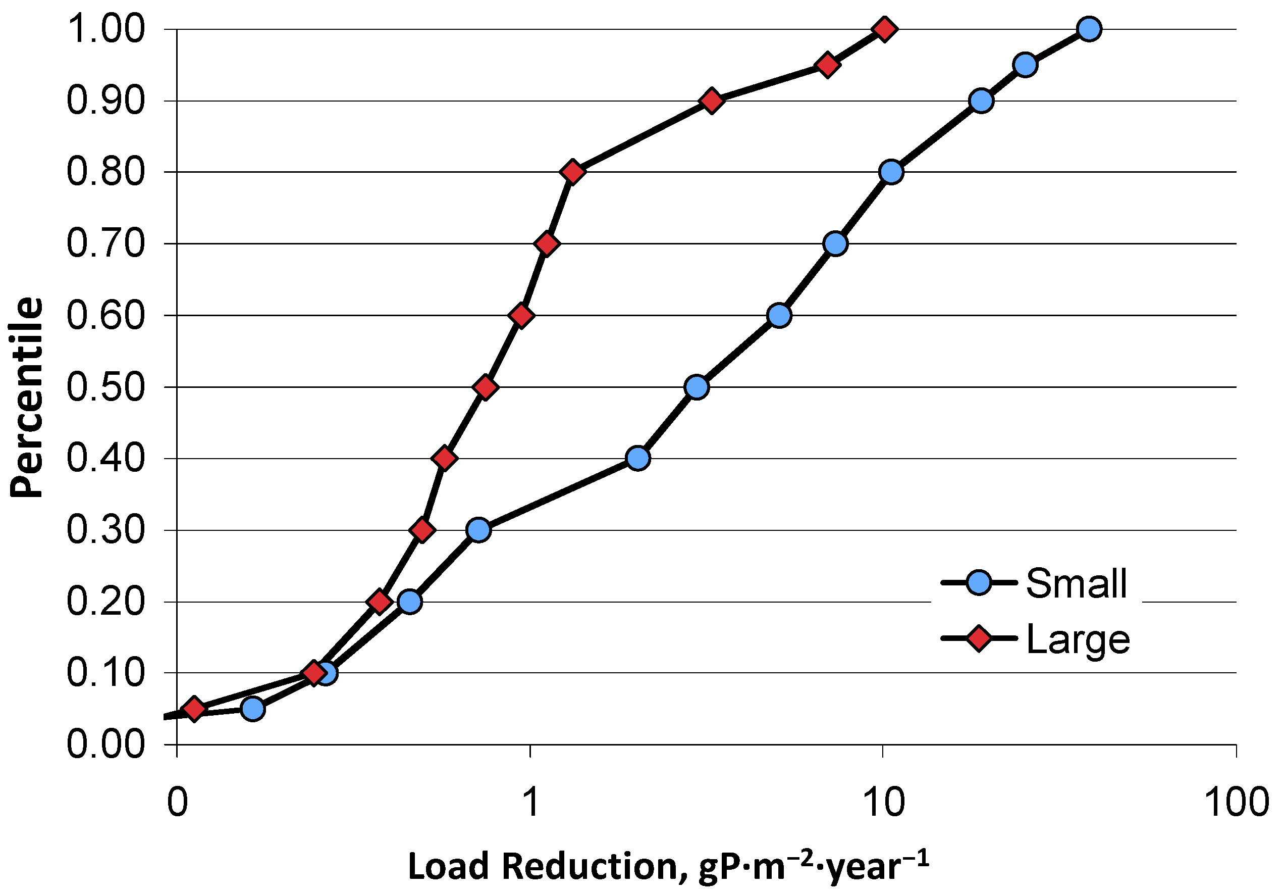
Figure 3.
Distributions of P removal rate coefficients for large (N = 43) and small (N = 87) constructed wetlands. A plateau concentration of 6 mgP·m−3 has been used. Large wetlands are assumed to have a distribution of detention times represented by eight tanks in series, and for the small dataset three tanks in series.
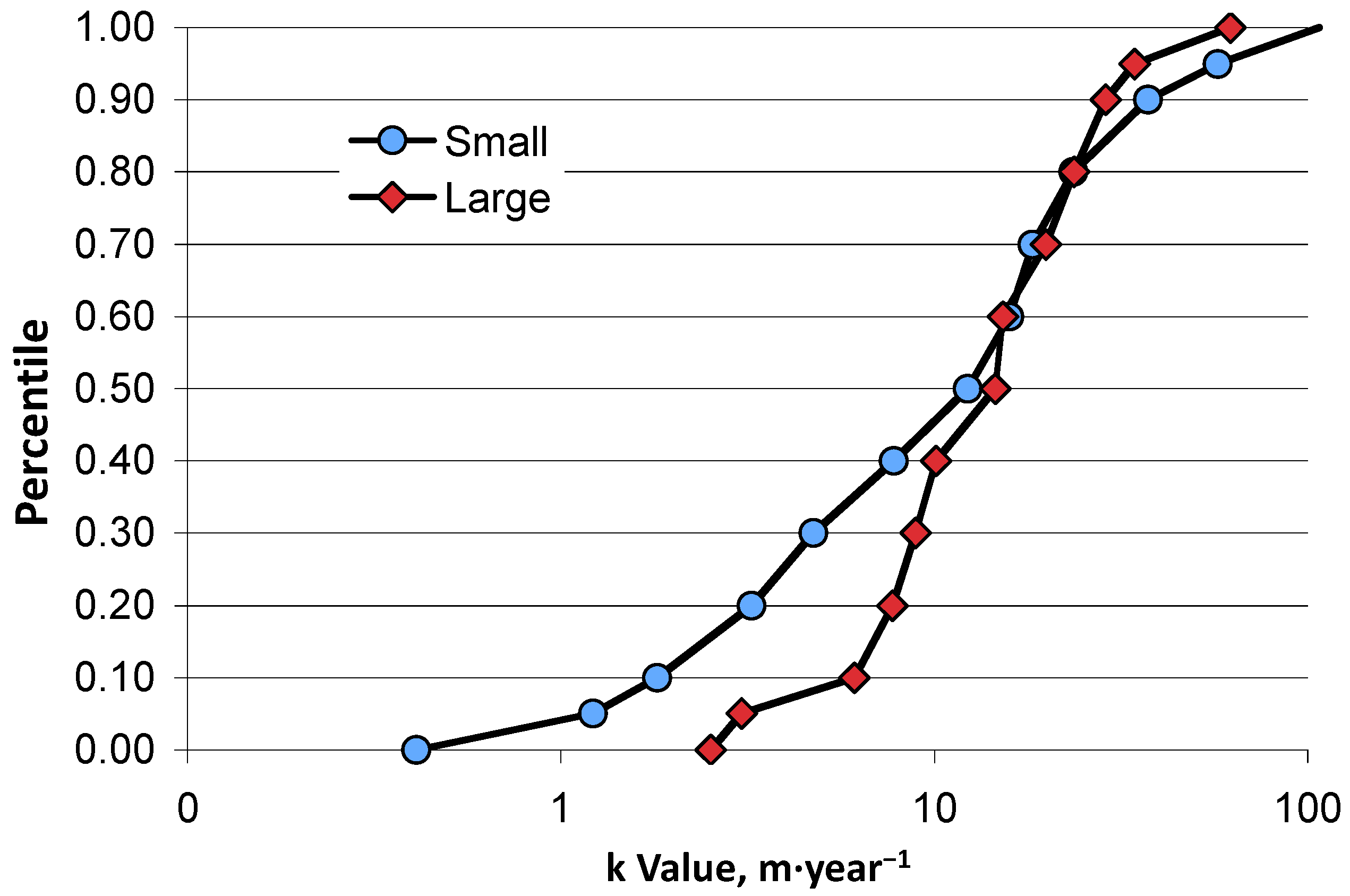
Figure 4.
Weekly average flow entering STA1West over a two year POR (period of record) (2011–2013). The mean daily flow was 0.42 ha3·day−1. Flow occurred on 30% of the days, at a mean rate of 1.38 ha3·day−1.
Figure 4.
Weekly average flow entering STA1West over a two year POR (period of record) (2011–2013). The mean daily flow was 0.42 ha3·day−1. Flow occurred on 30% of the days, at a mean rate of 1.38 ha3·day−1.
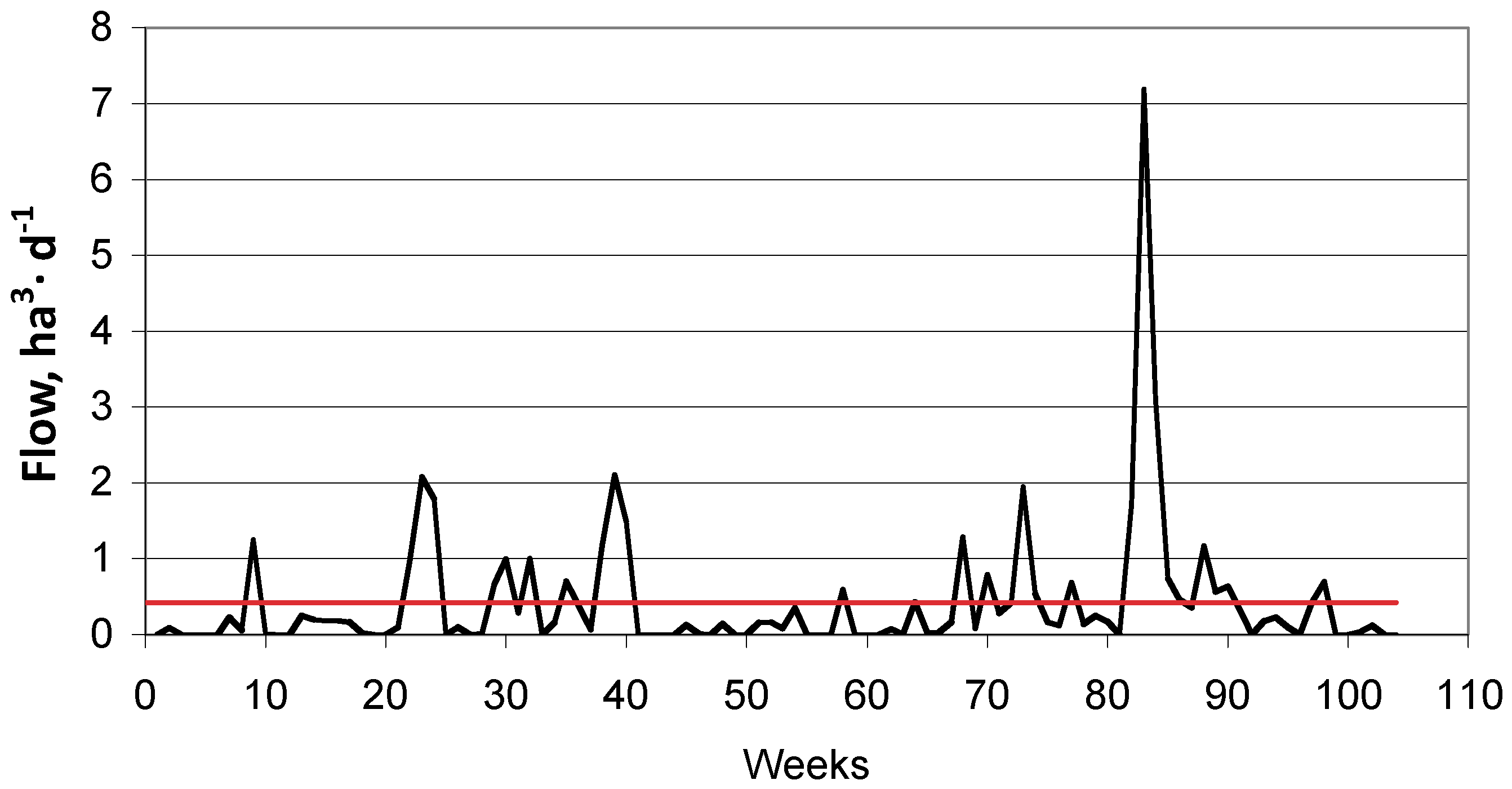
Figure 5.
Average monthly water depths for three large P-control wetlands. ENRP C1 (N = 5 years) contained emergent vegetation and was operated at nearly constant flow and depth. STA2 C1 (N = 8 years) fosters submerged aquatic vegetation and, therefore, was kept hydrated in the dry season. STA56 FW7 (N = 8 years) contains emergent vegetation, but was not kept hydrated in the dry season.

Figure 6.
Monthly performance of the ENRP over a four-year POR. The average hydraulic loading was 2.4 cm/day. PP (particulate) and Dissolved phosphorus (DP) are reduced in all months. Overall TP reduction is slightly less in the first six months of the year (73%) and slightly greater in the second six months (82%).

Figure 7.
Monthly performance of the Apopka Wetlands over a ten-year POR. The average hydraulic loading was 10.3 cm/day. PP is reduced in all months, but dissolved P is increased. Overall TP reduction is greater in the first six months of the year (34%, and much less in the second six months (2%).
Figure 7.
Monthly performance of the Apopka Wetlands over a ten-year POR. The average hydraulic loading was 10.3 cm/day. PP is reduced in all months, but dissolved P is increased. Overall TP reduction is greater in the first six months of the year (34%, and much less in the second six months (2%).
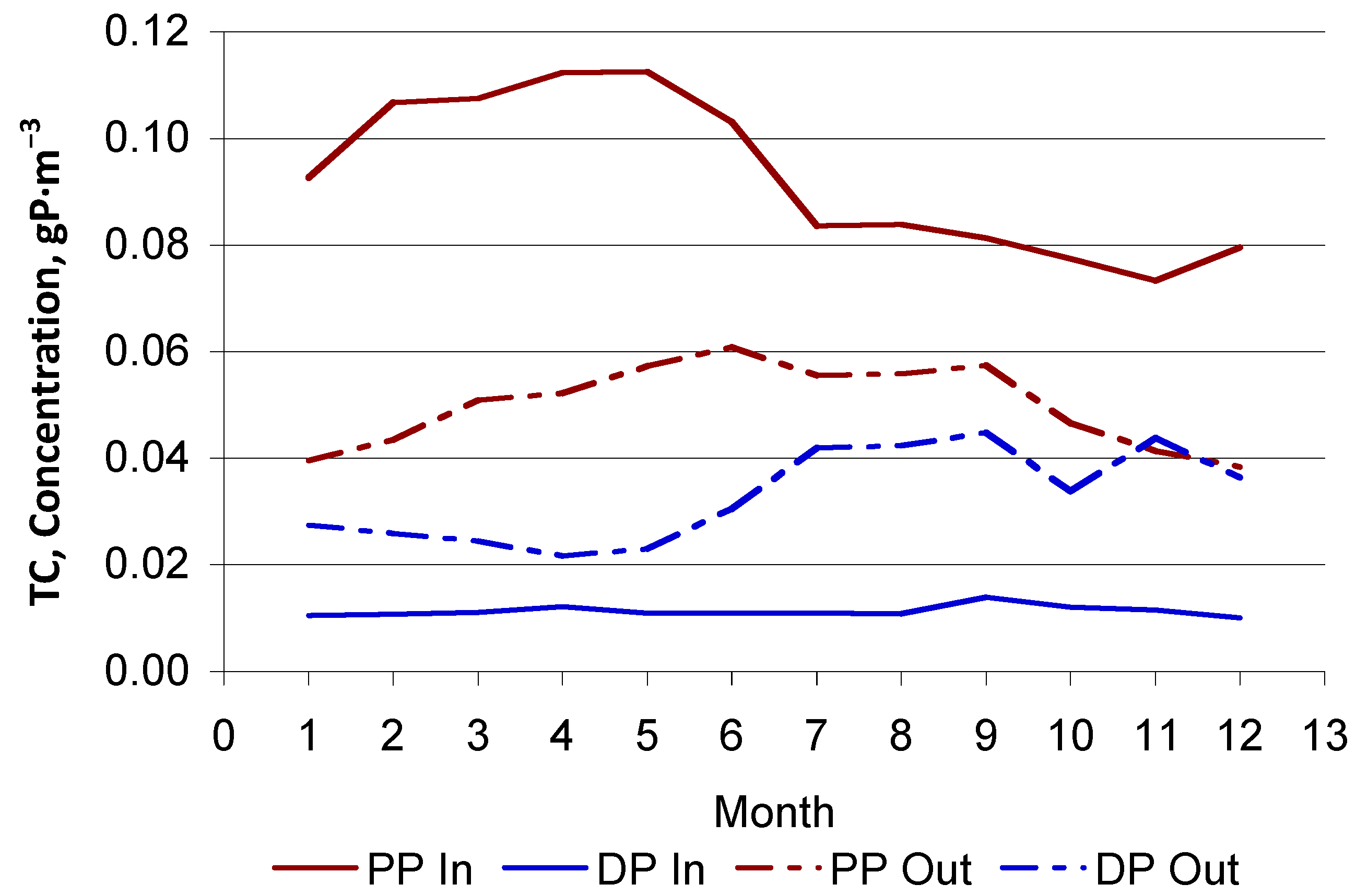
Figure 8.
The dependence of the rate coefficient on the fraction EAV in SAV–EAV (submerged aquatic vegetation–emergent aquatic vegetation) stormwater wetlands.
Figure 8.
The dependence of the rate coefficient on the fraction EAV in SAV–EAV (submerged aquatic vegetation–emergent aquatic vegetation) stormwater wetlands.
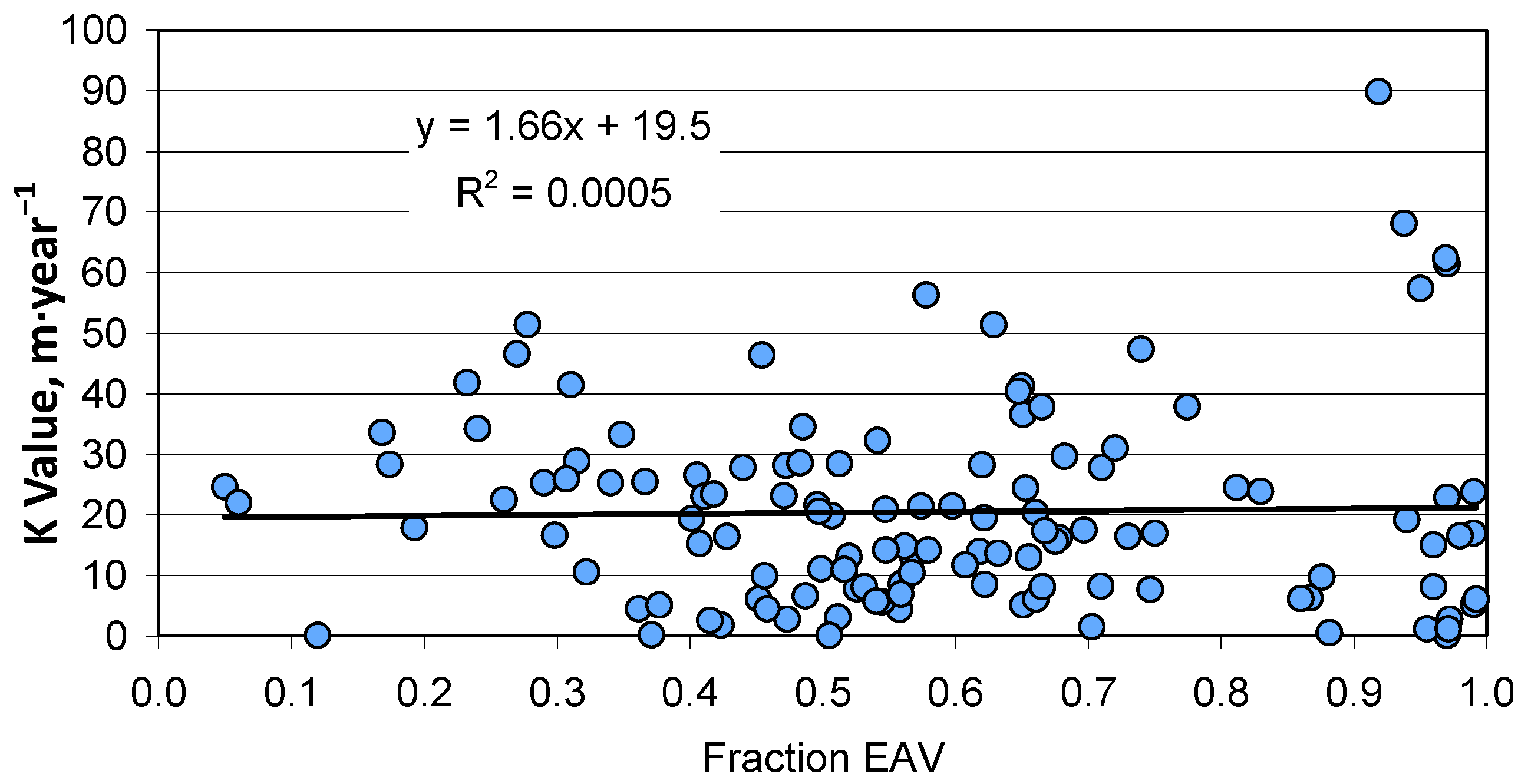
Figure 9.
The development of cattail cover in STA1E Cell 5 (231 ha). Flow-through began in October 2005. The site was a citrus grove prior to wetland construction.
Figure 9.
The development of cattail cover in STA1E Cell 5 (231 ha). Flow-through began in October 2005. The site was a citrus grove prior to wetland construction.
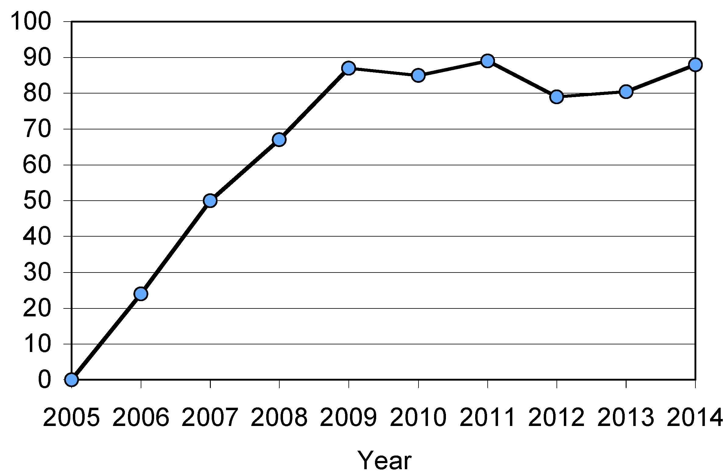
Figure 10.
Startup of STA1W Cell 5, beginning18 March 1999.
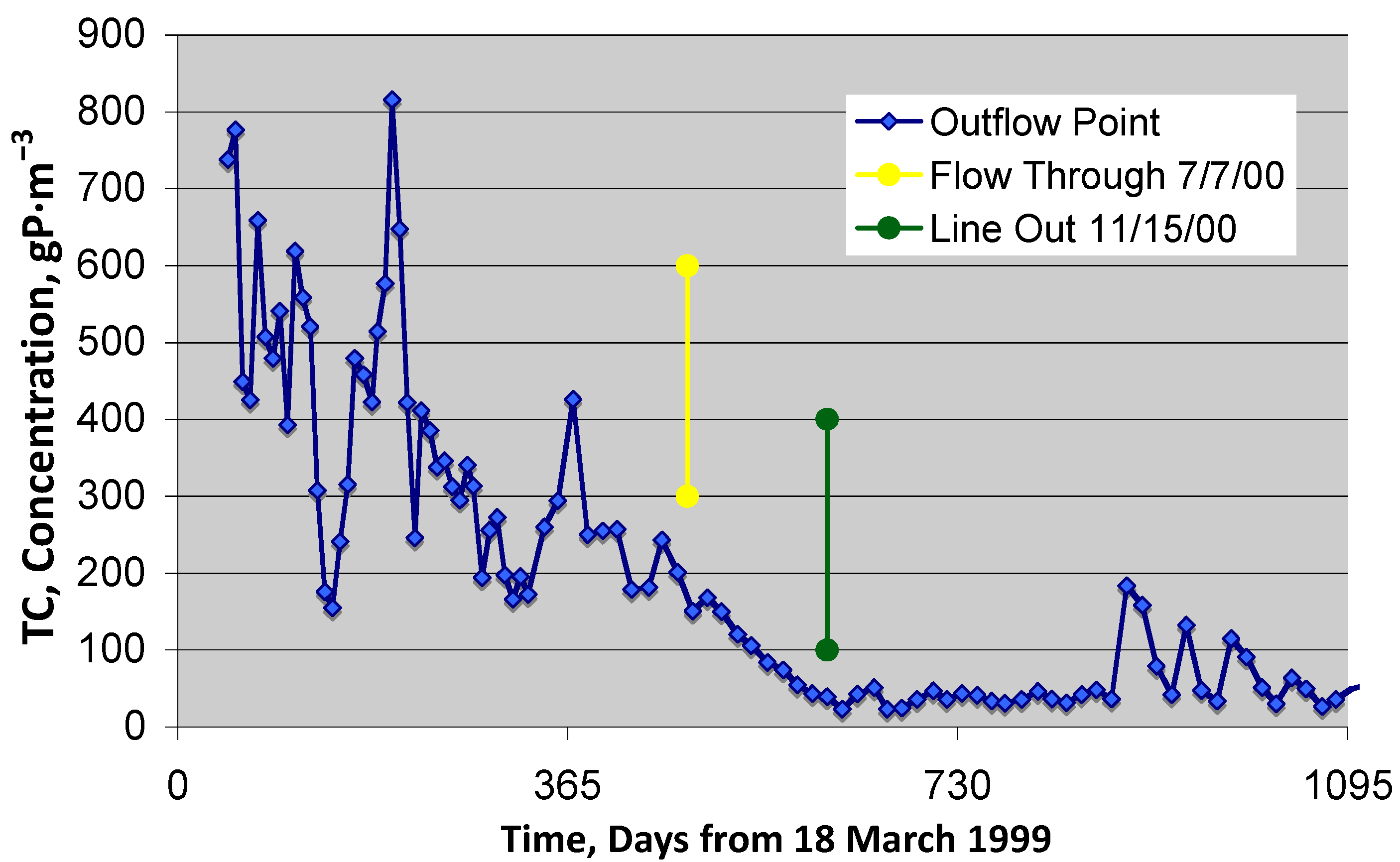
Figure 11.
Startup rate coefficients for the Shannon Wetland. Operations began in June 2003.

Figure 12.
Relative concentration reductions (CR) over the course of the year for six steady flow large P wetlands (OEW, Boney, Titusville, ENRP, Lakeland, Shannon). Data have been normalized by the long-term mean CR for each wetland. Error bars are the average standard deviation for all months.
Figure 12.
Relative concentration reductions (CR) over the course of the year for six steady flow large P wetlands (OEW, Boney, Titusville, ENRP, Lakeland, Shannon). Data have been normalized by the long-term mean CR for each wetland. Error bars are the average standard deviation for all months.

Figure 13.
Concentration reductions (CR) over the course of the year for the four Apopka steady flow large P wetlands. Error bars are the average standard deviation for all months.
Figure 13.
Concentration reductions (CR) over the course of the year for the four Apopka steady flow large P wetlands. Error bars are the average standard deviation for all months.
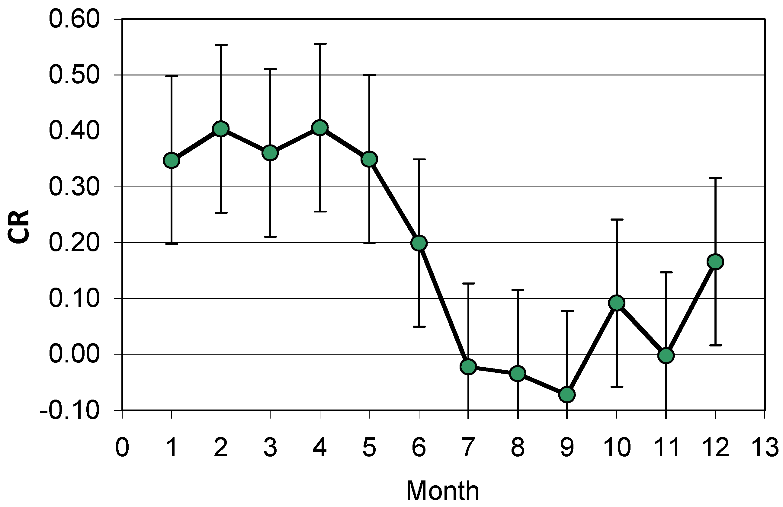
Figure 14.
Relative k-values over the course of the year for five STA large P wetlands (STA2C1, STA2C2, STA2C3, STA34 East, STA34 West). Data have been normalized by the long-term mean K-value for each wetland. Error bars are the average standard deviation for all months.
Figure 14.
Relative k-values over the course of the year for five STA large P wetlands (STA2C1, STA2C2, STA2C3, STA34 East, STA34 West). Data have been normalized by the long-term mean K-value for each wetland. Error bars are the average standard deviation for all months.
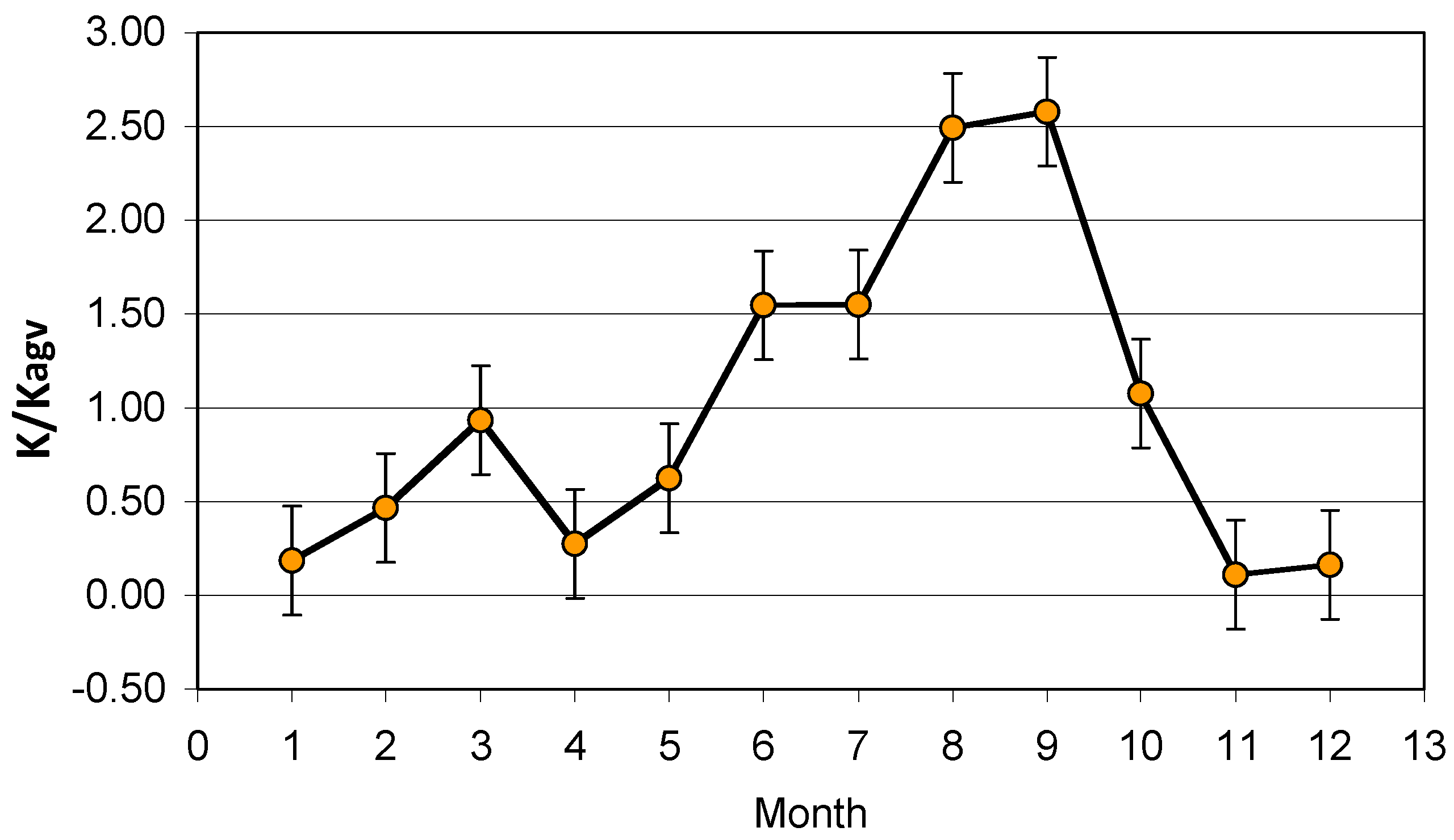
Figure 15.
Variability of outlet TP concentrations at Boney Marsh. The mean TP values are means for the designated month. (Source: unpublished data from South Florida Water Management District (SFWMD)).
Figure 15.
Variability of outlet TP concentrations at Boney Marsh. The mean TP values are means for the designated month. (Source: unpublished data from South Florida Water Management District (SFWMD)).
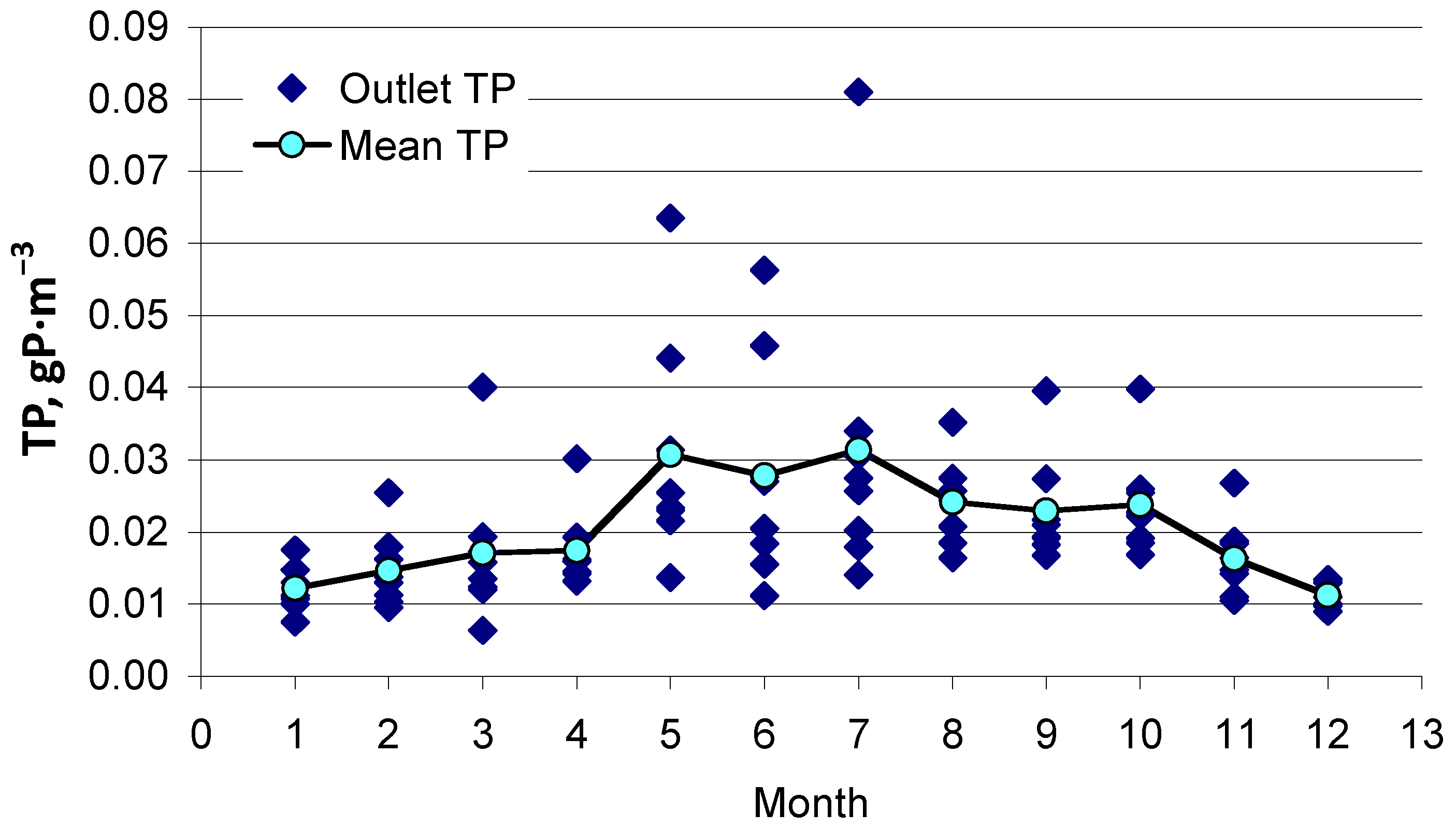
Figure 16.
Transect data and the kC* model for 28 grid transects for STA2C3 taken over five years. The data were flow-weighted. The hydraulic loading rates decrease as the location moves along the transect from inflow to outflow. Shown for comparison are the annual input/output flow-weighted concentration reductions for the five-year period. The model parameters are: K = 44.4 m/year, and C* = 6 μg/L, as co-determined by nonlinear regression. R2 = 0.977.

Figure 17.
Relative monthly rate coefficients (K/Kavg) versus the relative hydraulic loading (q/qavg) for five STA wetlands. Also shown are four flow groups of transect rate coefficients for STA2C3. (q = hydraulic loading, cm/day).
Figure 17.
Relative monthly rate coefficients (K/Kavg) versus the relative hydraulic loading (q/qavg) for five STA wetlands. Also shown are four flow groups of transect rate coefficients for STA2C3. (q = hydraulic loading, cm/day).
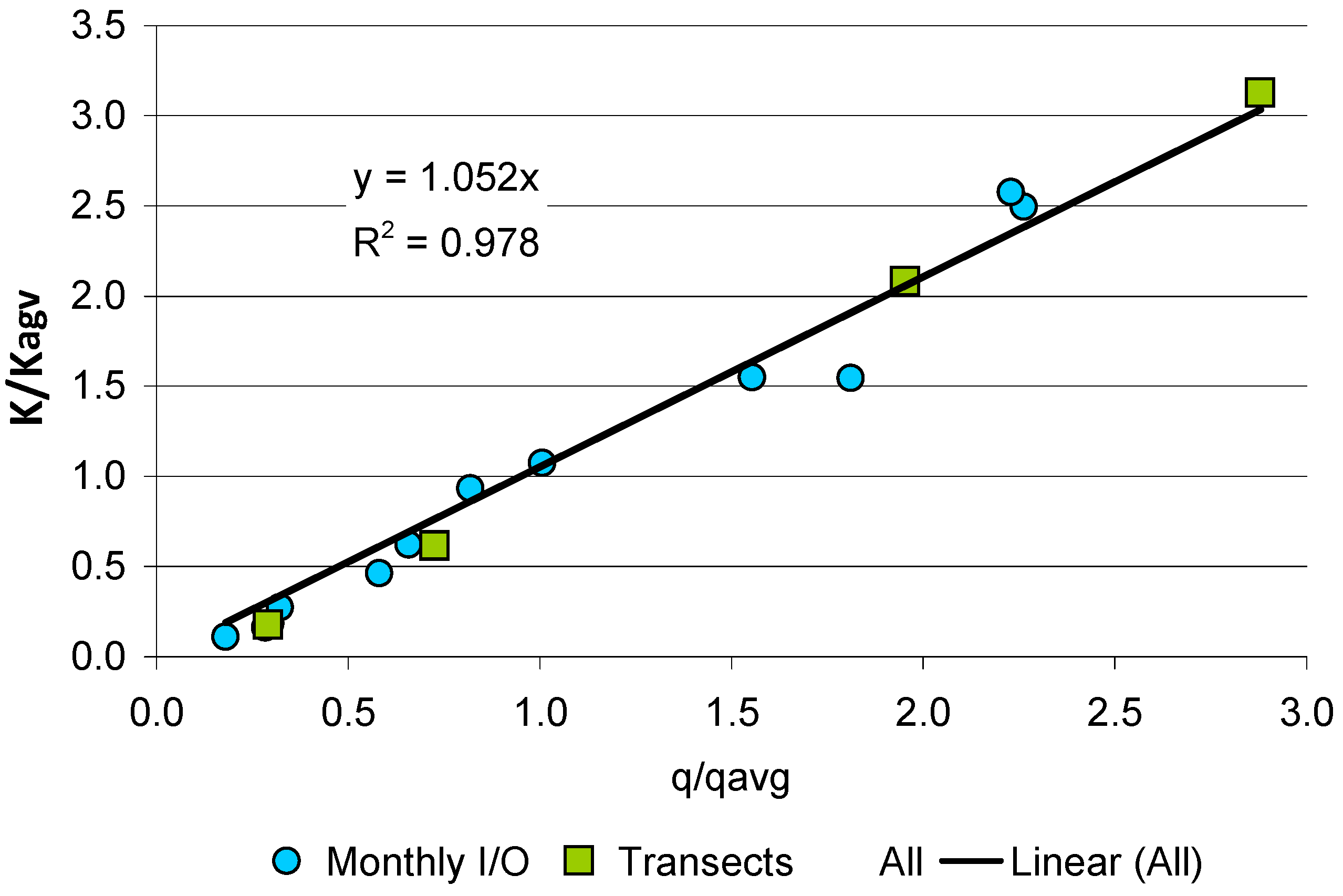
Figure 18.
Time progression of inlet and outlet TP concentrations for the OEW system.


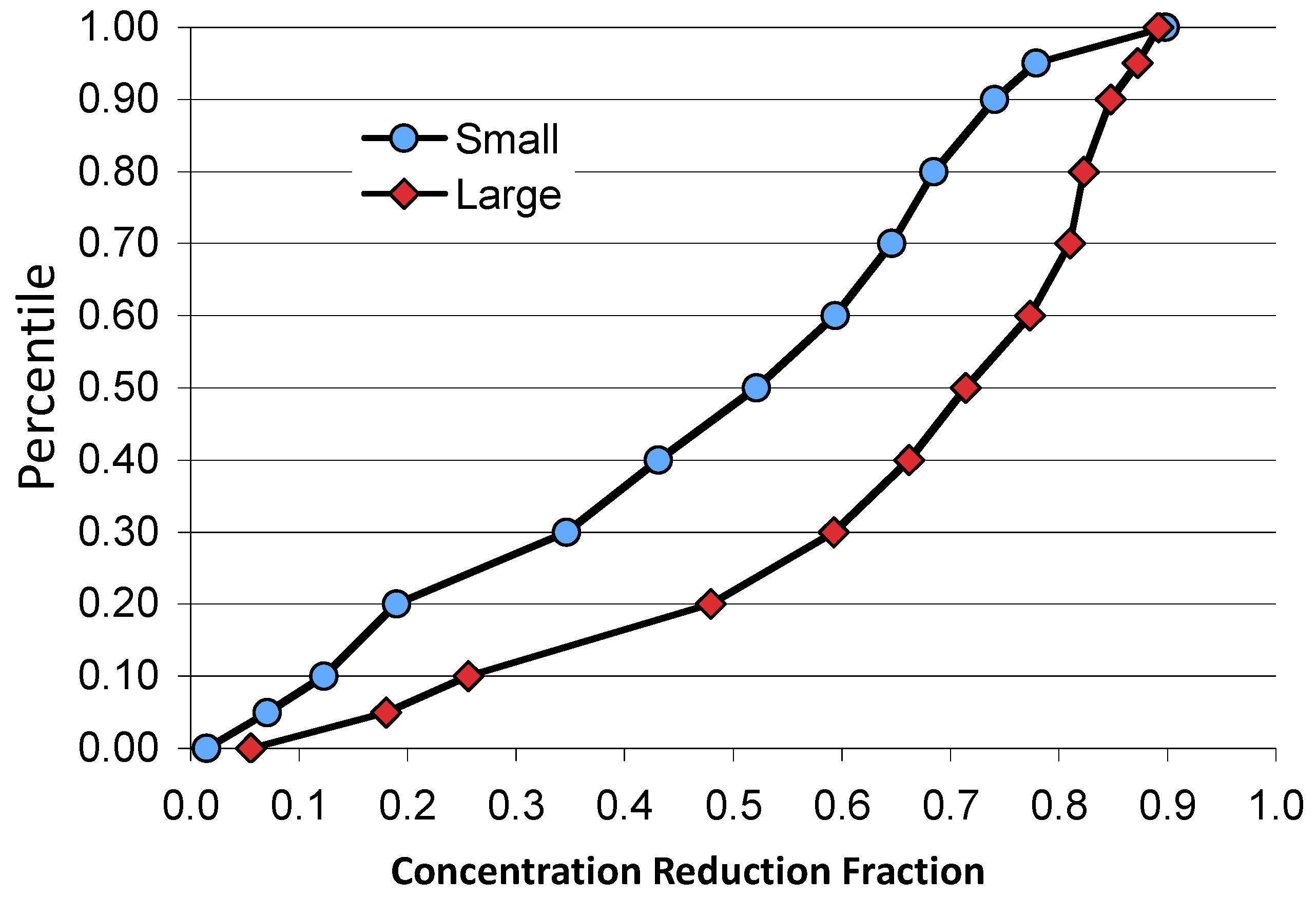
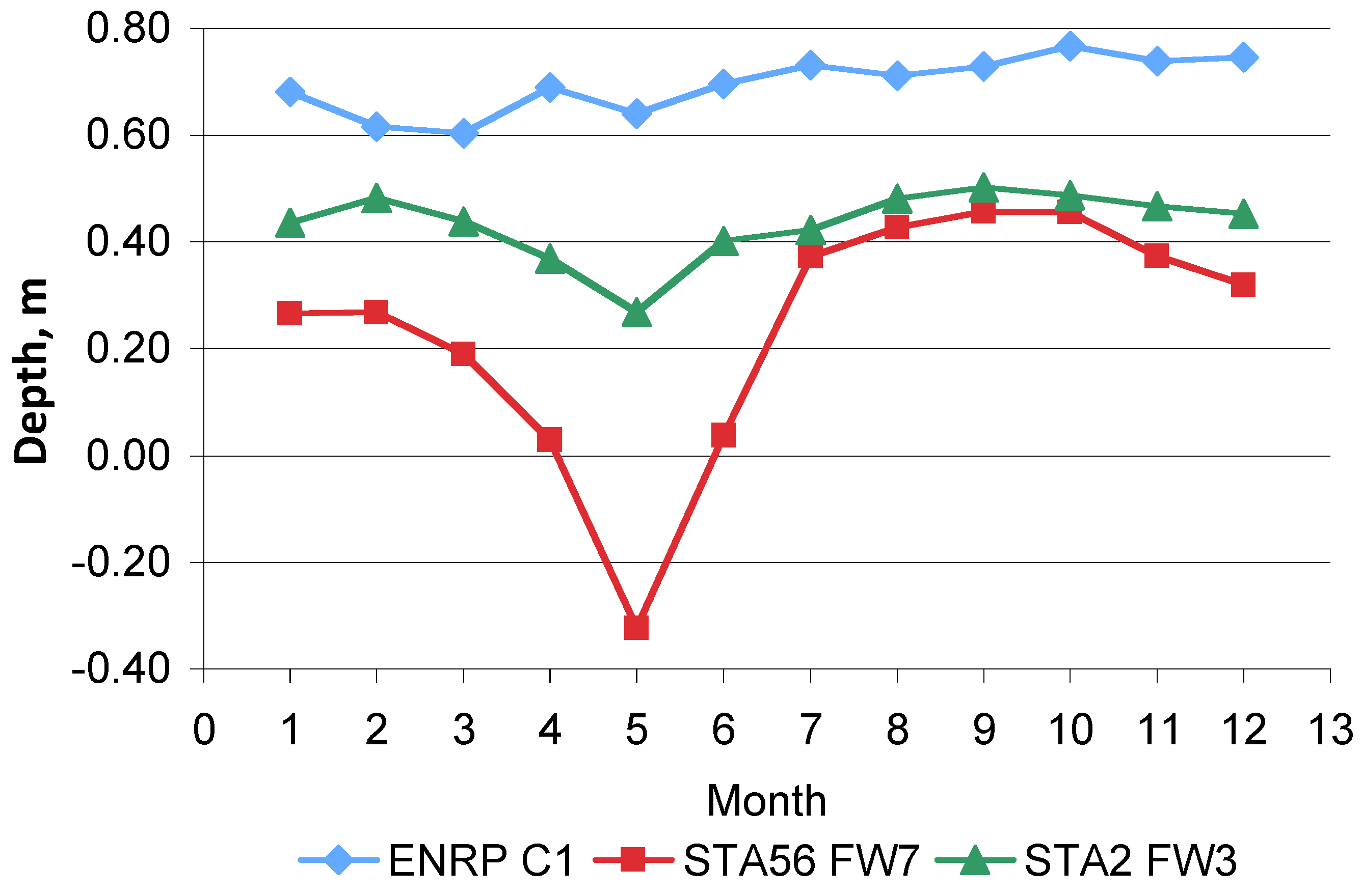
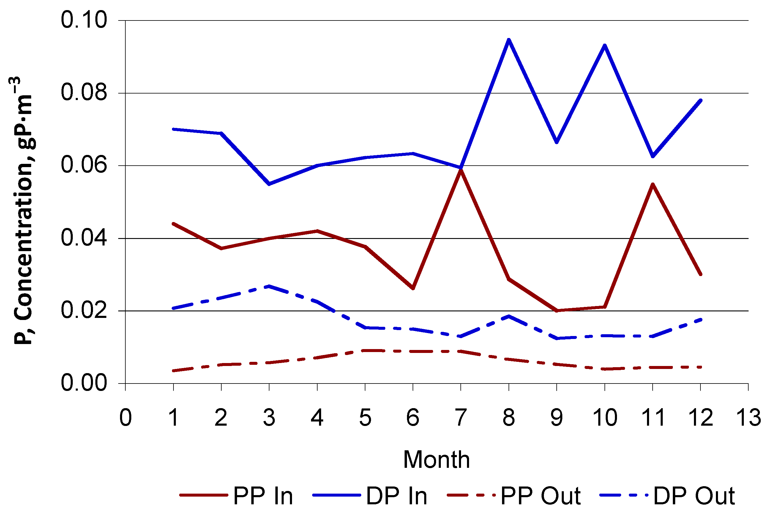
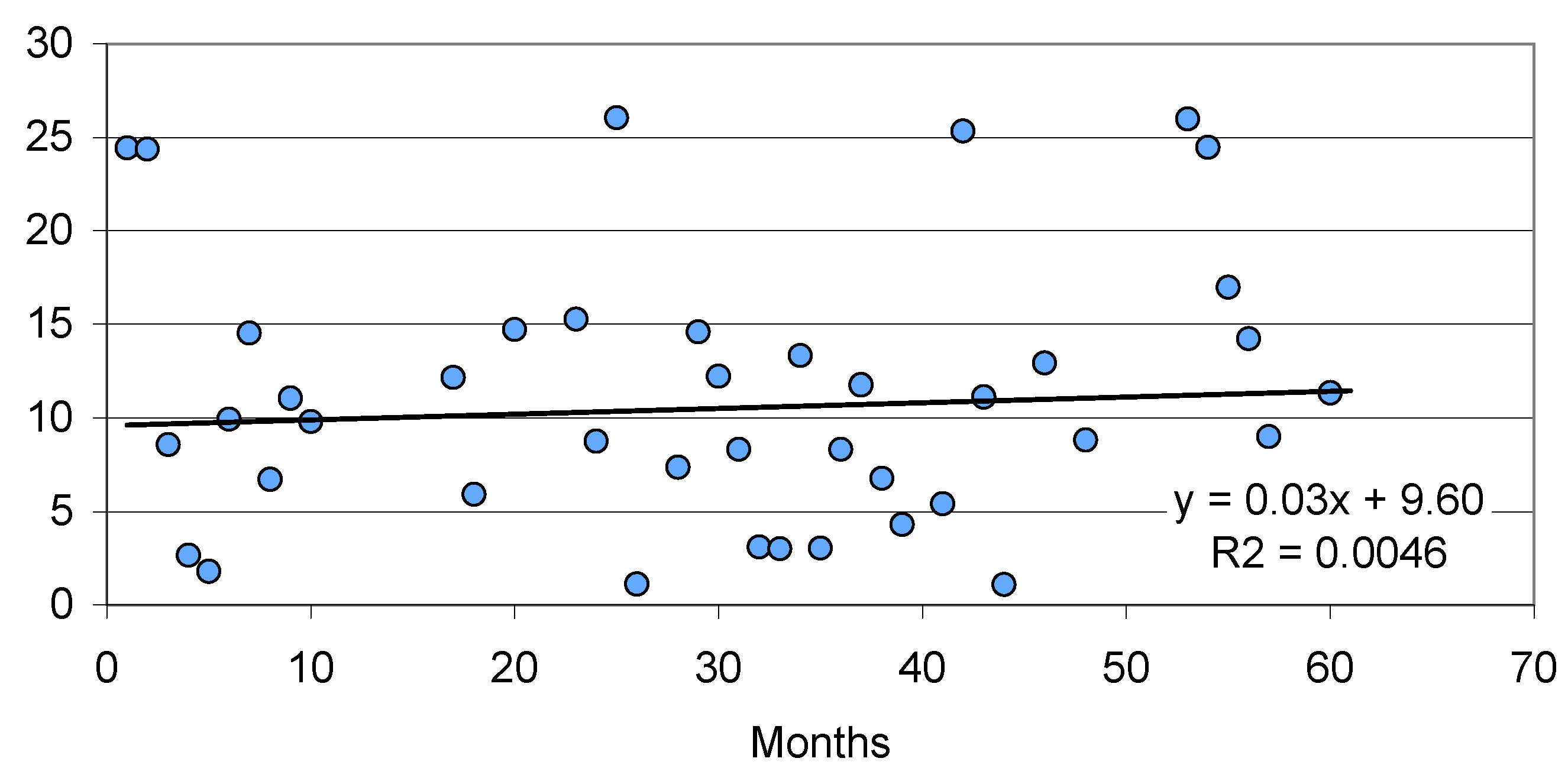
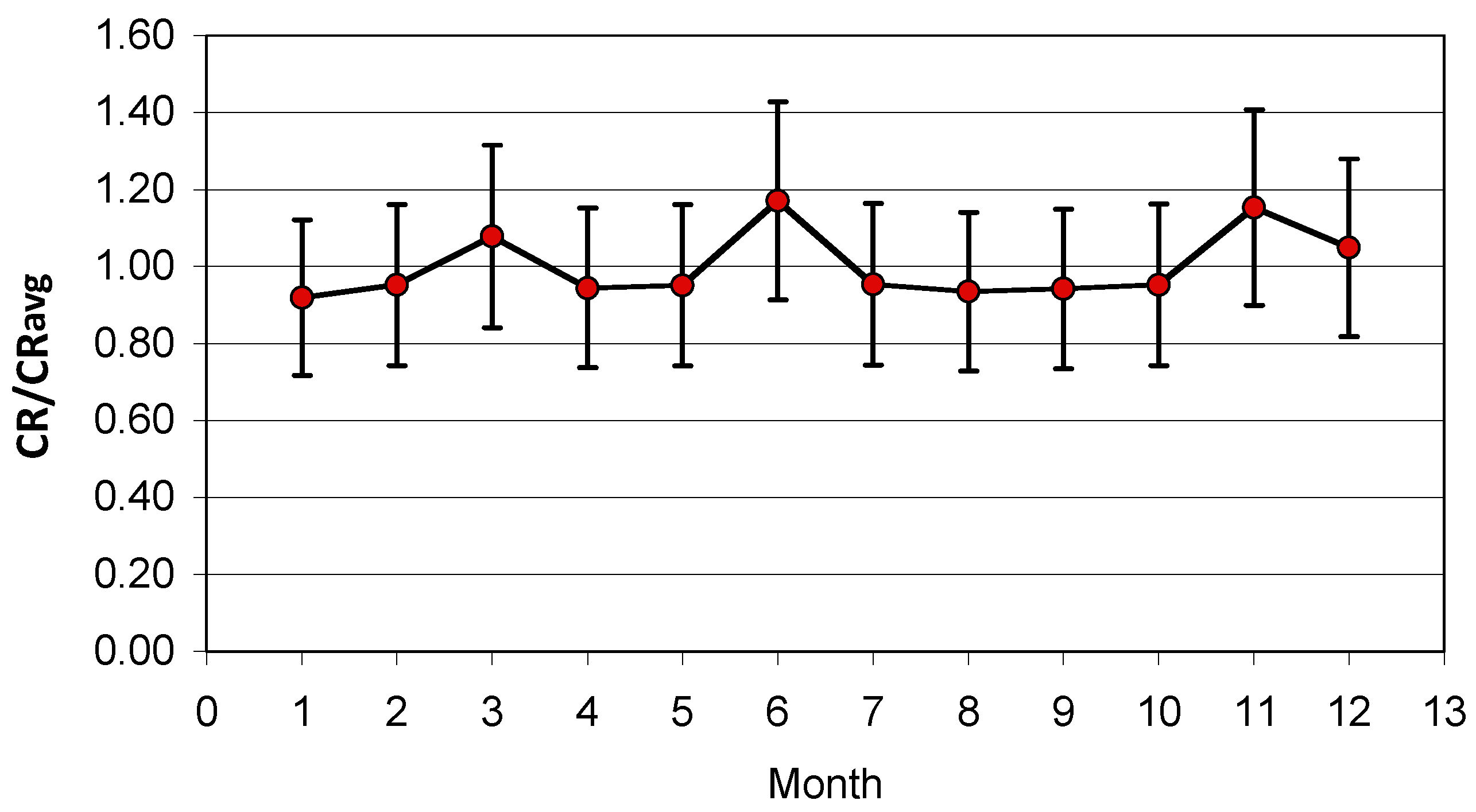
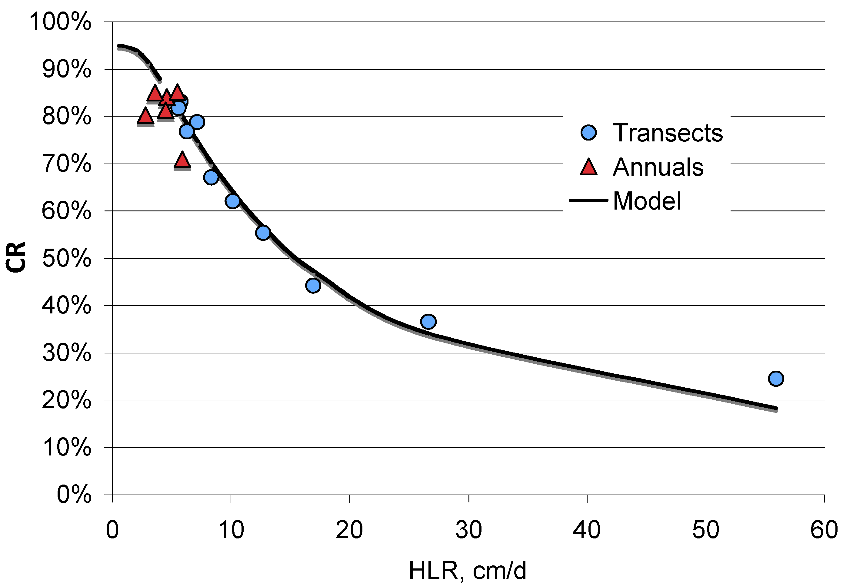
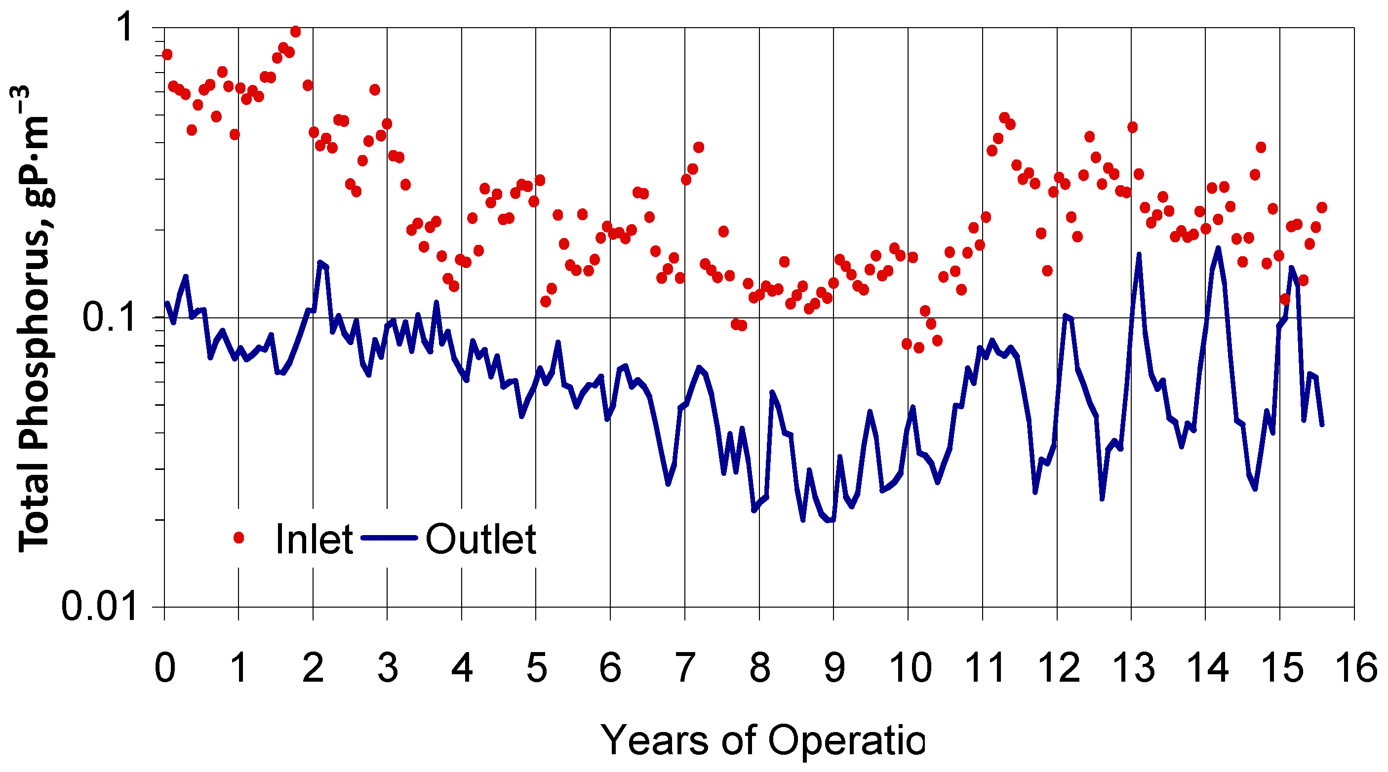
Table 1.
Large constructed wetlands treating phosphorus. Columbia and Lakeland do not specifically target phosphorus.
| Site | State/Country | System | Area | Cells | Start | Operating | Data | Ref. |
|---|---|---|---|---|---|---|---|---|
| ha | Year | Years | Years | |||||
| Columbia | MO | Columbia | 53 | 23 | 1994 | 23 | 14 | [21] |
| Lakeland | FL | Lakeland | 354 | 7 | 1987 | 30 | 12 | [22] |
| Balaton | Hungary | Feneki Pond | 1600 | 2 | 1992 | 25 | [11] | |
| Venice | Italy | Fusina | 100 | 6 | 2011 | 6 | [23] | |
| Portage la Prairie | Manitoba | Delta | 50 | 10 | 1980 | 37 | 10 | [8] |
| Putrajaya | Malaysia | Putrajaya | 197 | 23 | 1998 | 19 | 1 | [24] |
| Seagoville | TX | East Fork | 745 | 24 | 2009 | 8 | 1 | [25] |
| Melbourne | FL | Viera | 81 | 5 | 2002 | 15 | [26] | |
| Okeechobee Co. | FL | Nubbin Slough | 313 | 2 | 2013 | 4 | 1 | [27] |
| Martin Co. | FL | Lakeside Ranch | 691 | 8 | 2013 | 4 | [27] | |
| Okeechobee Co. | FL | Taylor Creek | 48 | 2 | 2010 | 7 | 3 | [27] |
| Tarrant | TX | Shannon | 171 | 4 | 2002 | 15 | 6 | [28] |
| Balaton | Hungary | Hidvegi Pond | 1800 | 2 | 1985 | 32 | 5 | [11] |
| Orange Co. | FL | OCESA | 56 | 4 | 1987 | 30 | 5 | [10] |
| Orlando | FL | OEW | 481 | 17 | 1987 | 30 | 13 | [29] |
| Boney Marsh | FL | West | 49 | 1 | 1976 | 41 | 11 | [7] |
| Apopka | FL | B1 | 73.1 | 1 | 1990 | 27 | 10 | [30] |
| Apopka | FL | B2 | 49.2 | 1 | 1990 | 27 | 10 | [30] |
| Apopka | FL | C1 | 77.9 | 1 | 1990 | 27 | 10 | [30] |
| Apopka | FL | C2 | 76.2 | 1 | 1990 | 27 | 10 | [30] |
| Titusville | FL | Blue Heron | 101 | 6 | 1997 | 20 | 7 | [31] |
| Palm Beach Co. | FL | ENRP | 1508 | 5 | 1994 | 5 | 5 | [32] |
| Palm Beach Co. | FL | STA1E East | 436 | 2 | 2005 | 12 | 2 | [33] |
| Palm Beach Co. | FL | STA1E Central | 782 | 3 | 2005 | 12 | 10 | [33] |
| Palm Beach Co. | FL | STA1E West | 796 | 3 | 2005 | 12 | 10 | [33] |
| Palm Beach Co. | FL | STA1W East | 875 | 3 | 2000 | 17 | 14 | [33] |
| Palm Beach Co. | FL | STA1W West | 552 | 3 | 2000 | 17 | 12 | [33] |
| Palm Beach Co. | FL | STA1W North | 1211 | 2 | 2000 | 17 | 16 | [33] |
| Palm Beach Co. | FL | STA2 FW1 | 742 | 1 | 2000 | 17 | 14 | [33] |
| Palm Beach Co. | FL | STA2 FW2 | 957 | 1 | 2000 | 17 | 15 | [33] |
| Palm Beach Co. | FL | STA2 FW3 | 926 | 1 | 2000 | 17 | 15 | [33] |
| Palm Beach Co. | FL | STA2 FW4 | 2415 | 3 | 2009 | 8 | 7 | [33] |
| Palm Beach Co. | FL | STA2 FW5 | 1208 | 2 | 2013 | 4 | 3 | [33] |
| Palm Beach Co. | FL | STA3/4 East | 2611 | 2 | 2004 | 13 | 11 | [33] |
| Palm Beach Co. | FL | STA3/4 Central | 2157 | 2 | 2004 | 13 | 11 | [33] |
| Palm Beach Co. | FL | STA3/4 West | 1815 | 2 | 2004 | 13 | 11 | [33] |
| Palm Beach Co. | FL | STA3/4 PSTA | 40 | 1 | 2008 | 9 | 8 | [33] |
| Hendry Co. | FL | STA5/6 FWY 1 | 975 | 2 | 1999 | 18 | 16 | [33] |
| Hendry Co. | FL | STA5/6 FWY 2 | 834 | 2 | 1999 | 18 | 16 | [33] |
| Hendry Co. | FL | STA5/6 FWY 3 | 775 | 2 | 2008 | 9 | 6 | [33] |
| Hendry Co. | FL | STA5/6 FWY 4 | 754 | 2 | 2012 | 5 | 3 | [33] |
| Hendry Co. | FL | STA5/6 FWY 5 | 1065 | 2 | 2012 | 5 | 3 | [33] |
| Hendry Co. | FL | STA5/6 FWY 6 | 766 | 2 | 2013 | 4 | 6 | [33] |
| Hendry Co. | FL | STA5/6 FWY 7 | 250 | 1 | 1997 | 20 | 13 | [33] |
| Hendry Co. | FL | STA5/6 FWY 8 | 98 | 1 | 1997 | 20 | 14 | [33] |
| Median | 2.0 | 15 | 10 |
| System | HLR | TP In | TP Out | CR | PLR | k |
|---|---|---|---|---|---|---|
| cm·day−1 | gP·m−3 | gP·m−3 | % | gP·m−2·year−1 | m·year−1 | |
| Columbia | 13.30 | 2.550 | 2.410 | 0.05 | 6.67 | 2.76 |
| Lakeland | 1.02 | 5.080 | 3.030 | 0.40 | 7.63 | 1.99 |
| Taylor Creek | 9.00 | 0.321 | 0.241 | 25% | 10.10 | 9.80 |
| Shannon | 5.45 | 0.888 | 0.539 | 39% | 6.94 | 10.3 |
| Hidvegi Pond | 2.76 | 0.544 | 0.232 | 0.57 | 3.14 | 9.2 |
| OCESA | 0.97 | 0.210 | 0.040 | 0.81 | 0.40 | 6.9 |
| OEW | 5.61 | 0.280 | 0.106 | 0.62 | 3.56 | 21.7 |
| Boney West | 2.16 | 0.051 | 0.019 | 0.63 | 0.25 | 9.7 |
| Apopka B1 | 9.88 | 0.110 | 0.076 | 0.31 | 1.40 | 15.6 |
| Apopka B2 | 11.76 | 0.095 | 0.071 | 0.26 | 1.40 | 14.5 |
| Apopka C1 | 10.20 | 0.109 | 0.088 | 0.19 | 1.16 | 8.8 |
| Apopka C2 | 9.34 | 0.102 | 0.095 | 0.07 | 0.77 | 2.5 |
| Blue Heron | 0.79 | 0.288 | 0.049 | 0.83 | 0.69 | 6.0 |
| ENRP | 3.11 | 0.108 | 0.022 | 0.80 | 0.97 | 23.6 |
| STA1E East | 2.52 | 0.091 | 0.013 | 0.86 | 0.63 | 27.50 |
| STA1E Central | 2.55 | 0.114 | 0.030 | 0.81 | 0.81 | 21.03 |
| STA1E West | 1.90 | 0.173 | 0.086 | 0.64 | 0.58 | 7.92 |
| STA1W East | 2.65 | 0.164 | 0.041 | 0.81 | 1.07 | 16.01 |
| STA1W West | 3.61 | 0.156 | 0.037 | 0.77 | 1.08 | 23.73 |
| STA1W North | 3.16 | 0.186 | 0.060 | 0.84 | 1.48 | 23.66 |
| STA2 FW1 | 3.15 | 0.093 | 0.012 | 0.89 | 0.94 | 61.90 |
| STA2 FW2 | 4.32 | 0.107 | 0.027 | 0.76 | 1.12 | 36.66 |
| STA2 FW3 | 4.06 | 0.095 | 0.018 | 0.82 | 1.13 | 33.31 |
| STA2 FW4 | 1.47 | 0.093 | 0.022 | 0.71 | 0.43 | 14.71 |
| STA2 FW5 | 0.51 | 0.045 | 0.020 | 0.53 | 0.05 | 2.98 |
| STA3/4 East | 2.42 | 0.085 | 0.016 | 0.81 | 0.51 | 20.87 |
| STA3/4 Central | 2.22 | 0.069 | 0.019 | 0.71 | 0.33 | 14.84 |
| STA3/4 West | 3.07 | 0.066 | 0.016 | 0.77 | 0.50 | 29.62 |
| STA3/4 PSTA | 4.63 | 0.019 | 0.011 | 0.40 | 0.12 | 16.05 |
| STA5/6 FWY 1 | 2.55 | 0.153 | 0.070 | 0.53 | 0.55 | 8.22 |
| STA5/6 FWY 2 | 2.25 | 0.196 | 0.079 | 0.66 | 0.73 | 12.15 |
| STA5/6 FWY 3 | 0.57 | 0.278 | 0.038 | 0.85 | 0.48 | 6.30 |
| STA5/6 FWY 4 | 0.60 | 0.257 | 0.033 | 0.87 | 0.49 | 6.30 |
| STA5/6 FWY 5 | 0.36 | 0.190 | 0.032 | 0.83 | 0.23 | 3.09 |
| STA5/6 FWY 6 | 2.20 | 0.177 | 0.052 | 0.70 | 0.78 | 12.46 |
| STA5/6 FWY 7 | 1.94 | 0.107 | 0.033 | 0.72 | 0.36 | 14.98 |
| STA5/6 FWY 8 | 2.26 | 0.082 | 0.035 | 0.55 | 0.30 | 8.45 |
| Median | 2.55 | 0.114 | 0.038 | 0.71 | 0.77 | 12.5 |
Table 3.
Phosphorus speciation in water entering and leaving the stormwater treatment areas (STAs) during a POR ending in 2007 (gP·m−3).
| System | Location | TP | SRP | DOP | PP | DP |
|---|---|---|---|---|---|---|
| STA1E | In | 0.143 | 0.059 | 0.013 | 0.070 | 0.073 |
| STA1W | In | 0.158 | 0.085 | 0.009 | 0.064 | 0.094 |
| STA2 | In | 0.097 | 0.068 | 0.006 | 0.022 | 0.075 |
| STA34 | In | 0.088 | 0.043 | 0.008 | 0.036 | 0.052 |
| STA56 | In | 0.059 | 0.011 | 0.007 | 0.041 | 0.019 |
| Median | 0.097 | 0.059 | 0.008 | 0.041 | 0.073 | |
| STA1E | Out | 0.023 | 0.005 | 0.010 | 0.007 | 0.015 |
| STA1W | Out | 0.074 | 0.043 | 0.008 | 0.023 | 0.051 |
| STA2 | Out | 0.021 | 0.011 | 0.004 | 0.006 | 0.015 |
| STA34 | Out | 0.019 | 0.004 | 0.005 | 0.010 | 0.009 |
| STA56 | Out | 0.017 | 0.006 | 0.004 | 0.006 | 0.011 |
| Median | 0.021 | 0.006 | 0.005 | 0.007 | 0.015 |
Table 4.
Phosphorus accumulation in soils and removed from water in STAs. Accretion and P accumulation were measured at a small number of locations in each wetland for soil cores taken in 2009 [64]. The P removed is calculated from annual performance data for the water entering and leaving the wetlands, which typically spanned the majority of the operating history.
| System | Wetland | Accretion | P Accumulation | P Removed | |||
|---|---|---|---|---|---|---|---|
| cm·year−1 | gP·m−2·year−1 | gP·m−2·year−1 | |||||
| mean | stdev | mean | stdev | mean | stdev | ||
| STA1W | East | 0.97 | 0.31 | 1.20 | 0.61 | 1.21 | 0.65 |
| STA1W | West | 0.90 | 0.22 | 1.47 | 0.36 | 1.64 | 1.01 |
| STA1W | North | 1.10 | 0.54 | 2.05 | 1.24 | 1.15 | 0.97 |
| STA2 | FW1 | 1.00 | 0.26 | 1.00 | 0.13 | 0.99 | 0.36 |
| STA2 | FW2 | 1.00 | 0.26 | 1.60 | 0.41 | 1.34 | 0.52 |
| STA2 | FW3 | 1.20 | 0.40 | 2.50 | 1.00 | 1.14 | 0.49 |
| STA3/4 | East | 1.70 | 0.66 | 2.55 | 0.94 | 0.90 | 0.44 |
| STA3/4 | Central | 1.75 | 0.78 | 4.65 | 2.85 | 0.69 | 0.58 |
| mean | 1.20 | 2.13 | 1.13 | ||||
| stdev | 0.34 | 1.17 | 0.29 | ||||
| Wetlands | Years | Percentile | |||
|---|---|---|---|---|---|
| 50% | 80% | 90% | 95% | ||
| ENRP | 4 | 1.00 | 1.24 | 1.35 | 1.44 |
| Lakeland | 7 | 1.00 | 1.23 | 1.46 | 1.51 |
| Boney | 8 | 0.92 | 1.15 | 1.55 | 1.73 |
| Titusville | 7 | 0.89 | 1.39 | 1.77 | 2.00 |
| OEW | 10 | 0.72 | 1.39 | 2.07 | 2.50 |
| Apopka | 9 | 0.82 | 1.26 | 1.64 | 1.86 |
| Median | 0.91 | 1.25 | 1.59 | 1.79 | |
Table 6.
Time trends in annual concentration reduction (CR), rate coefficients (k), and P load removed (PLR) for large P wetlands. Two natural wetlands are included because of their long history. Slopes are in percent per year.
| Site | System | Years | CR | k | PLR | |||
|---|---|---|---|---|---|---|---|---|
| Trend | Slope | R2 | Slope | R2 | Slope | R2 | ||
| Boney | West | 11 | 1.8 | 0.114 | 2.4 | 0.094 | 3.9 | 0.193 |
| OEW | Stratum 4 | 12 | −1.0 | 0.032 | 4.7 | 0.061 | 3.1 | 0.050 |
| Titusville | 7 | 0.4 | 0.003 | 4.5 | 0.014 | −12.0 | 0.167 | |
| Lakeland | Cells 1–4 | 12 | −1.1 | 0.019 | 2.7 | 0.041 | −4.4 | 0.130 |
| Shannon | 6 | 0.2 | 0.190 | 7.5 | 0.347 | 8.1 | 0.670 | |
| Bayou Marcus | Natural | 14 | −3.0 | 0.289 | 0.1 | 0.000 | 12.9 | 0.697 |
| Houghton Lake | Natural | 26 | −0.7 | 0.334 | −0.2 | 0.004 | −0.2 | 0.002 |
| Apopka | B1 | 9 | 8.6 | 0.563 | 4.0 | 0.115 | 2.8 | 0.036 |
| Apopka | B2 | 9 | 2.6 | 0.026 | −0.7 | 0.001 | −0.7 | 0.000 |
| Apopka | C1 | 9 | 4.1 | 0.001 | −2.6 | 0.003 | −2.9 | 0.003 |
| Apopka | C2 | 7 | −16.4 | 0.087 | 4.4 | 0.003 | 9.0 | 0.013 |
| Median Steady | 9 | 0.2 | 0.087 | 2.7 | 0.014 | 2.8 | 0.050 | |
| STA1E | Central | 10 | −2.7 | 0.102 | −7.3 | 0.076 | −11.4 | 0.217 |
| West | 10 | 4.1 | 0.014 | 4.5 | 0.021 | −17.1 | 0.162 | |
| STA1W | East | 14 | 2.9 | 0.333 | −2.4 | 0.041 | −4.0 | 0.143 |
| West | 12 | 1.5 | 0.317 | 0.8 | 0.012 | 0.3 | 0.000 | |
| North | 16 | 5.2 | 0.500 | 6.1 | 0.323 | 2.3 | 0.039 | |
| STA2 | FW1 | 12 | 0.5 | 0.072 | 4.8 | 0.095 | 0.7 | 0.004 |
| FW2 | 13 | 0.3 | 0.019 | 1.2 | 0.030 | −0.3 | 0.001 | |
| FW3 | 13 | 1.3 | 0.185 | −0.7 | 0.010 | 0.5 | 0.003 | |
| FW4 | 7 | 2.2 | 0.034 | −0.2 | 0.000 | −13.4 | 0.200 | |
| STA34 | East | 11 | −0.6 | 0.093 | −3.4 | 0.074 | −15.4 | 0.497 |
| Central | 11 | −1.3 | 0.092 | −9.1 | 0.198 | −23.4 | 0.391 | |
| West | 11 | 0.0 | 0.000 | 5.6 | 0.254 | 0.0 | 0.000 | |
| PSTA | 8 | −7.5 | 0.507 | −2.4 | 0.021 | −1.4 | 0.007 | |
| STA56 | FW1 | 16 | 8.7 | 0.534 | 1.9 | 0.014 | −7.6 | 0.113 |
| FW2 | 16 | 5.0 | 0.166 | −0.1 | 0.000 | −12.4 | 0.247 | |
| FW3 | 6 | 0.2 | 0.005 | 10.7 | 0.142 | 0.1 | 0.000 | |
| FW6 | 6 | 5.7 | 0.549 | −14.3 | 0.274 | −16.9 | 0.772 | |
| FW7 | 13 | −1.0 | 0.066 | −11.8 | 0.528 | −8.7 | 0.081 | |
| FW8 | 14 | 1.0 | 0.010 | −19.8 | 0.312 | −9.4 | 0.134 | |
| Median Storm | 12 | 1.0 | 0.093 | −0.2 | 0.074 | −7.6 | 0.113 | |
| Global Median | 11 | 0.5 | 0.0925 | 0.5 | 0.041 | −1.1 | 0.097 | |
© 2016 by the author; licensee MDPI, Basel, Switzerland. This article is an open access article distributed under the terms and conditions of the Creative Commons Attribution (CC-BY) license (http://creativecommons.org/licenses/by/4.0/).
Share and Cite
MDPI and ACS Style
Kadlec, R.H. Large Constructed Wetlands for Phosphorus Control: A Review. Water 2016, 8, 243. https://doi.org/10.3390/w8060243
AMA Style
Kadlec RH. Large Constructed Wetlands for Phosphorus Control: A Review. Water. 2016; 8(6):243. https://doi.org/10.3390/w8060243
Chicago/Turabian StyleKadlec, Robert H. 2016. "Large Constructed Wetlands for Phosphorus Control: A Review" Water 8, no. 6: 243. https://doi.org/10.3390/w8060243
Note that from the first issue of 2016, this journal uses article numbers instead of page numbers. See further details here.