Numerical Simulations of Suspended Sediment Dynamics Due to Seasonal Forcing in the Mekong Coastal Area

Abstract

The Mekong River is ranked as the 8th in terms of water discharge and as the 10th in terms of sediment load in the world. During the last 4500 years, its delta prograded more than 250 km to the south due to a tremendous amount of sediments deposited, and turned from a “tide-dominated” delta into a “wave-and-tide dominated” delta. This study aims at completing our knowledge on the fate of sediments that may be stored in estuarine or coastal systems, or dispersed over the continental shelf and slope. Sediment transport in the Mekong River Delta (MRD) coastal area was studied by numerical simulations using the Delft3D model. The model configuration was calibrated and validated from data collected in situ during 4 periods from 2012 to 2014. Then, 50 scenarios corresponding to different wave conditions (derived from the wave climate) and river discharge values typical of low flow and flood seasons enabled us to quantify the dispersal patterns of fluvial sediments close to the mouths and along the coast. Sediments mostly settled in the estuary and close to the mouths under calm conditions, and suspended sediment with higher concentrations extend further offshore with higher waves. Waves from the Southeast enhanced the concentration all along the MRD coastal zone. Waves from the South and Southwest induced coastal erosion, higher suspended sediment concentrations in front of the southern delta, and a net transport towards the Northeast of the delta. Because of episodes of Southern and Southwestern waves during the low flow season, the net alongshore suspended sediment transport is oriented Northeastward and decreases from the Southwestern part of the coastal zone (~960 × 10³ t yr⁻¹) to the Northeastern part (~650 × 10³ t yr⁻¹).

1. Introduction

Rivers originating from the Tibetan plateau and the Himalayas (Ganges, Brahmaputra, Yellow River, Yangtze, Mekong, Irrawady, Red River, Pearl River) are huge providers of sediments to the ocean at global scale [1]. However, recent human activities have severely altered their sediment discharge, mainly as a consequence of artificial impoundments, and also by activities such as groundwater pumping, irrigation, dredging, and deforestation [2]. At a global scale, around 53% of river sediment flux is now potentially trapped in reservoirs [3], and this reduction dramatically affects deltas [4]. For example, in Asia, sediment discharge decreased by 87% (from 1200 to 150 × 10⁶ t yr⁻¹) over a 40 year period in the Yellow River (Huanghe) [5,6] and by 61% (from 119 to 46 × 10⁶ t yr⁻¹) in the Red River after the Hoa Binh dam settlement [7].

Sediment dynamics have considerable impacts, not only in terms of geomorphology but also in terms of geochemical cycles [8,9], biogeochemistry [10], microbiology [11], fate of metal contamination [12], benthic environment, coral reefs and seagrass communities ([13] and references therein). Sediment budgets are thus of interest for many interdisciplinary studies [14].

Seasonally, the sediment discharge, transport and deposition in the Asian deltas are strongly affected by the variations in precipitation, wind and waves induced by the monsoons [15,16]. The monsoons highly influence coastal geomorphology of these deltas, which experience rapid changing shorelines. Understanding the influences of monsoons is essential for predicting changes in sedimentary environment and coastal geomorphology [16].

The Mekong River delta (MRD) is amongst the third largest delta plain in the world, with 16–20 million inhabitants in its Vietnamese part (density of ~460 people km⁻², [17]). It covers an area of 62,500 km² between Phnom Penh in the Cambodian lowlands and the southern Vietnamese coast [18]. The MRD lies entirely within three meters above sea level.

Recent studies focused on sediment variability in the Mekong River [19,20], on sedimentation in the Lower Mekong River [21,22], within the distributaries [23], and along the MRD coast at depths > 5 m [24]. The concentration of surface suspended matter in the Mekong River plume was shown to decrease by ~5% per year during the period 2002–2012 from the analysis of MERIS satellite data [25]. However, little is known on the fate of sediments reaching the sea that may be stored in estuarine or coastal systems, or dispersed over the continental shelf and slope ([26] and references therein).

With a tidal range up to 3 m in spring tide, sediment dynamics within the Mekong distributaries is strongly affected by tidal oscillations. From in situ measurements, Wolanski et al. [27,28] sketched a conceptual model of the present-day sediment dynamics in the Bassac estuary (the southern main distributary of the Mekong River), completed by Hein et al. [29]: most of the sediment brought by the River is deposited in the shallow coastal waters of depth <20 m (corresponding to the subaqueous delta) in the flood season, while a net flux of particles occurs upstream in the estuary during the low flow season. Alongshore, numerical simulations by Hein et al. [29] have shown that deposition dominates over the annual cycle directly off the mouths of the Mekong branches, where erosion prevails throughout the year in shallow waters to the North and to the South (along the Cape), while erosion and deposition alternate further offshore with the seasonal cycle. Therefore, there are specific needs to quantitatively assess the dispersal patterns of fluvial sediments close to the mouths and along the coasts for management purposes.

This paper aims at complementing the previous studies in the coastal area along the Mekong River delta. The variability of sediment transport along the delta is examined during the low flow and flood seasons from numerical modeling, under 50 scenarios based on the wave climate (25 scenarios per season). The resulting numerical simulations are discussed in view of recent changes in sediment deposition and erosion along the delta coastline.

2. Materials and Methods

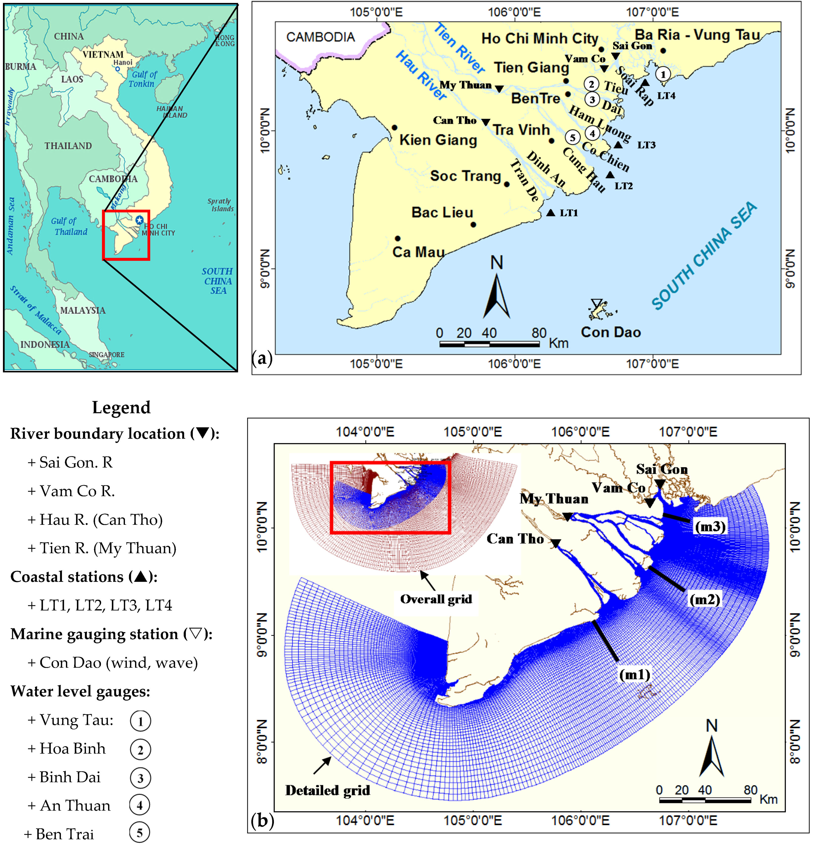
2.1. The Mekong River Delta (MRD)

2.1.1. The Mekong River

The Mekong River originates from the Tibetan plateau at elevations mostly >5000 m, then flows through six countries along a 4880-km course down to the South China Sea (East Sea of Vietnam), making it the 12th longest river in the world [22]. The Mekong River, which drains a basin area of ~795 × 10³ km² [19], was ranked as the 8th in terms of water discharge with an average flow of 15,000 m³·s⁻¹ [30] and as the 10th in terms of sediment load with an average value estimated to be 160 × 10⁶ t yr⁻¹ [31], corrected to 144 ± 36 × 10⁶ t yr⁻¹ over the last 3 k yr by Ta et al. [32].

The Mekong River water and sediment discharges are distributed amongst a network of two main distributaries which divide near Phnom Penh: the Mekong—called the Tiền River after entering Vietnam—to the North, and the Bassac—called the Hậu River in Vietnam—to the South. The Mekong (Tien) distributary divides itself into three main estuaries with Tieu and Dai mouths for the further North, Ham Luong for the central branch, and Co Chien and Cung Hau mouths for the further South. The Bassac (Hau) River divides mainly into the Tran De mouth and the Dinh An mouth (see Figure 1).

The Dong Nai–Saigon River system flows to the South China Sea just to the North of the MRD. The Saigon River is called Soai Rap River in its lower basin. The Vamco River is a tributary that joins the Soai Rap River just upstream of its mouth (Figure 1a).

During the last 4500 years, the MRD prograded more than 250 km to the southeast [18]. Approximately 3000 years ago, the prodelta was located near Ben Tre and Tra Vinh cities (see [32], their Figure 4). During this recent progradation (~3 k yr BP), the southern coast of the MRD became more sensitive to waves from the East and North-East during the dry season, and the MRD turned from a “tide-dominated delta” into a “tide-and-wave dominated” delta [32]. The continental shelf is very shallow (most of the plume flows over depths <10–15 m), the river mouths being located in a sedimental plain. Despite the low Coriolis number, the large freshwater discharge still creates a baroclinic coastal current flowing in the direction of the Kelvin wave [33].

2.1.2. Climate and Rainfall

The Mekong basin ranges from cool temperate to tropical climates. The Lower Mekong River basin is subject to a tropical climate that is characterized by a summer monsoon from the Southwest (from May to October) and a winter monsoon from the Northeast (from November to April). The wet season (from June to October) alternates with a dry season (November–May) and accounts for 85%–90% of the total yearly rainfall. In South Vietnam, the annual rainfall ranges between 1600 and 2000 mm [34,35]. Rainfall is higher (2000–2400 mm per year) in the Western region than in the Eastern (1600–1800 mm) and in the central delta (1200–1600 mm) [36]. According to the Vietnamese National Centre for Hydro-Meteorological Forecasts [37], 18 typhoons impacted on the MRD during the 52-year period of 1961–2012. Amongst them, 13 typhoons occurred recently, during the last 20 years (1992–2012).

2.1.3. Hydrological Regimes and Sediment Transport

The total water discharge of the Mekong is ~500 km³ yr⁻¹, of which 85% flows in flood season (from September to November) and 15% in low flow season (from December to August) [21,35]. In the delta, the flood season occurs later than the local rainy season, since the water flux mainly comes from the upper and central Mekong basin and is partially regulated by the dynamics of the Tonle Sap in Cambodia. Discharges at the Can Tho and My Thuan stations are almost the same, and vary between 25,000 m³·s⁻¹ in September-October and a minimum in April (typically 2000 m³·s⁻¹) [38]. The total suspended sediment discharge entering the delta is about 145 × 10⁶ t yr⁻¹, and the average sediment concentration in the river is about 60 mg·L⁻¹; maximum values can reach 500 mg·L⁻¹ in the wet season [39].

The suspended sediments in the distributaries of the Mekong are mostly composed of fine silt with about 15% clay [27].

The coastal current along the MRD shifts with the monsoon forcing; it is oriented Southwestward during the Northeast (or winter) monsoon and Northeastward during the Southwest (or summer) monsoon [40].

2.1.4. Tides

The MRD is affected by tides of a mixed diurnal and semi-diurnal character. Semi-diurnal lunar tide M2 and solar tide S2 amplitudes are up to 0.9 m and 0.5, respectively, while diurnal solar tide K1 and lunar tide O1 amplitudes are up to 0.7 m and 0.5 m, respectively, along the MRD [41]. The resulting amplitude is gradually decreasing from 3.8 m in the Northeast (NE) area to approximately 2 m in the Southwest (SW) along the Ca Mau peninsula [26].

Tidal mechanisms are key processes acting on water distribution in deltas and on sediment transport in estuaries (e.g., [42,43,44]). In the middle and lower estuaries, deposition is mainly driven by the dynamics of the turbidity maximum zone, whose presence and dynamics are governed by the coupling between river discharge and tidal propagation (e.g., tidal pumping and/or density gradients; [27,28,45,46]). In this study, tidal propagation within the estuaries is included in the numerical model and the tide is taken into account through its boundary conditions in the river mouths.

2.2. Data

Data used to set up, calibrate and validate the model are the following.

Bathymetry and coastline in the MRD coastal area were digitized from topography maps in VN2000 coordinates (national coordinate system of Vietnam corresponding to UTM projection with a WGS84 reference ellipsoid and specified local parameters) with scale 1:50,000 in the coastal zone and 1:25,000 in the estuary. These maps were published by the Department of Survey and Mapping in 2004, now belonging to the Ministry of Natural Resources and Environment of Vietnam. Bathymetry offshore was extracted from GEBCO-1/8 with 30 arc-second interval grid [47].

River water discharge and suspended sediment concentration (SSC) measured in the period 2007–2014 at My Thuan (Tien River) and Can Tho (Hau River) were used to set-up river boundary condition in these rivers. In the absence of gauging station in the Vamco River and Soai Rap River (to the North of the MRD), the averaged river discharges and SSCs in low flow and flood seasons provided by a previous project [48] were used to set up the river boundary conditions in these rivers.

Wind and wave data measured at Con Dao Island and Vung Tau were analyzed and used in the simulations. Data measured with interval of 6 hours in 2012, 2013 and 2014 were considered in this study for calibration/validation. Wave and wind average values over 20 years (1992–2013) from the wave climate [49] were considered along the MRD coastal zone to setup different scenarios of simulations.

Sea level elevations measured at Vung Tau, Hoa Binh, Binh Dai, An Thuan and Ben Trai stations (Figure 1a) were used for model calibration and validation. Moreover, measured sea level near the coast was analyzed to determine the harmonic constants of 8 tidal constituents (M2, S2, K2, N2, O1, K1, P1, Q1) to be imposed at sea boundaries in the refined grid. The tidal harmonics constants imposed offshore were extracted from FES2014 [50,51]. The World Ocean Atlas [52] with 0.25 degree-grid resolution was used for open sea boundary transport condition of the parent model.

Current velocity, grain size of bottom sediment and SSC were measured in the framework of the project “Interaction between hydrodynamics of the Bien Dong (East Sea of Vietnam) and Mekong River water” at 4 in situ stations (LT1, LT2, LT3 and LT4, see Figure 1a) in September 2013 (flood season) and April 2014 (low flow season). These data were used for model calibration and validation.

2.3. Modelling Strategy

2.3.1. The Delft3D Model

In this study, hydrodynamics (resulting from tides, currents and waves) and suspended sediment transport were simulated using the Delft3D-Flow module and the Delft3D-Wave module (based on the SWAN model). The Delft3D-Flow model developed by Deltares (Delft, The Netherlands) is a 3D modeling suite to investigate hydrodynamics, sediment transport and morphology, and water quality for fluvial, estuarine and coastal environment [53]. Delft3D solves the Reynolds-averaged Navier-Stokes equations, including the k-ε turbulence closure model, and applies a horizontal curvilinear grid with σ-layers for vertical grid resolution.

SWAN is used as wave model [54,55,56]. In the action balance equation (see e.g., [57]), the JONSWAP expression [58] is chosen to express the bottom friction dissipation, with the parameter C_jon = 0.067 m²·s⁻³ proposed by Bouws and Komen [59] for fully developed wave conditions in shallow water. The model from Battjes and Janssen [60] is used to model the energy dissipation in random waves due to depth-induced breaking waves.

2.3.2. Model Setup

The NESTING method (Delft3D-NESTHD) was used to create sea boundaries condition for a refined (child) grid within a coarse (parent or overall) model. The parent model grid is orthogonal, curvilinear with 210 × 156 grid cells. Horizontal grid size changes from 166 to 22,666 m (Figure 1b). Along the vertical, 4 layers in σ-coordinate are considered, each of them accounting for 25% of the water depth. Open sea boundary conditions of the overall model are provided by FES2004 and the World Ocean Atlas 2013.

The grid of the detailed model is also orthogonal curvilinear. Curvilinear grids are applied in the models to provide a high grid resolution in the area of interest and a low resolution elsewhere, thus saving computational effort. The model frame includes all the coastal zone of Ba Ria-Vung Tau to Ca Mau cape (Figure 1a) along circa 485 km in the long-shore direction and 100 km in the cross-shore direction. The horizontal grid encompasses 424 × 296 points with grid size between 44 m and 11,490 m. Along the vertical, 4 layers in σ-coordinate are considered, similar to the parent model. The hydrodynamics model takes into account the influences by water temperature, salinity, sediment transport and wave actions.

The model was setup and run for different periods of time, with time steps of 0.2 min (12 s). Its calibration and validation were performed during 4 periods: March–May 2012 (low flow season), August–October 2012 (flood season), September 2013 (flood season) and April 2014 (low flow season).

There are four open river boundaries: Soai Rap, Vamco, My Thuan and Can Tho (Figure 1b). The Soai Rap and Vamco boundaries belong to the Dong Nai–Saigon River catchment. River water discharge measured every hour in Can Tho and My Thuan stations were imposed as river boundary conditions. Others river boundaries were set to 546.9 m³·s⁻¹ (Soai Rap R.) and 52.5 m³·s⁻¹ (Vamco R.) in low flow season; 1310 m³·s⁻¹ in the Soai Rap River and 177.8 m³·s⁻¹ in the Vamco River in flood season. The averaged SSC values during flood tide and ebb tide at Can Tho and My Thuan stations were imposed as boundary condition for these two distributaries. SSC in Vamco and Soai Rap rivers were almost the same and considered in this study to be worth 55 mg·L⁻¹ in low flow season and 70 mg·L⁻¹ in flood season. At each river boundary, the same SSC values were imposed from the surface to the bottom.

The averaged water temperature and salinity values in the low flow and flood seasons were imposed at the river boundaries (T = 27.5 °C in low flow season and 27.2 °C in flood season; S = 0). Wind velocity and direction, which were measured every 6 h in Con Dao in the period 2012–2014, were imposed on the model. The wave module was setup with online coupling with hydrodynamics and sediment transport. Sea boundary conditions of the wave model were extracted from the wave climate [49].

The bottom roughness was specified by a spatial distribution of Manning (n) coefficients with values in the range 0.018–0.023 m^−1/3·s [61,62]. The background horizontal eddy viscosity and horizontal eddy diffusivity were considered to be, after calibration, equal to 8 m·s⁻². The Horizontal Large Eddy Simulation (HLES) sub-grid, which is integrated in Delf3D-Flow, is based on theoretical considerations presented by Uittenbogaard [63] and Van Vossen [64]. In this study, the HLES sub-grid was activated to add calculated results to background values. Two sediment fractions were simulated in the model: one non-cohesive and one cohesive.

Measured grain sizes of non-cohesive particles in the MRD coastal area range from 29 to 252 μm (average 113 μm) in flood season (September 2013) and from 15 to 262 μm (averaged 103 μm) in low flow season (April 2014). Therefore, median sand-sized particles of 113 μm and 103 μm were considered in our simulations in flood and low flow season, respectively. A specific density of 2650 kg·m⁻³ and dry bed density of 1600 kg·m⁻³ were considered; all other sand transport calibration parameters were kept at the default values proposed by Delft3D. Sand fraction transport was modeled with the van Rijn TR2004 formulation [65], which has been shown to successfully represent the movement of non-cohesive sediment ranging in size from 60 μm to 600 μm.

Previous observational studies in the Mekong estuary indicated that most of Mekong sediments are flocculated fine particles. In low flow season, measured flocsize was 30–40 μm with about 20%–40% of clay content in volume [28]. In the flood season, the flocsize was 50–200 μm with a 20%–30% clay content in volume [27]. For the cohesive sediments, if the bed shear stress is larger than a critical value, erosion is modeled following the Partheniades’ formulation [66], whereas if the bed shear stress is less than a critical value for deposition, Krone’s formula [67] is used to quantify the deposition flux. The parameters required to simulate the cohesive sediment transport include critical bed shear stresses for erosion τ_cre and deposition τ_crd, the erosion parameter M and the particle settling velocity w_s [68]. After calibration, τ_crd was set to 1000 N·m⁻², which effectively implied that deposition was a function of concentration and fall velocity [69]. τ_cre was set to 0.2 N·m⁻², and M was set to 2 × 10⁻⁵ kg·m⁻²·s⁻¹.

In salt water, cohesive sediments flocculate, the degree of flocculation depending on salinity. Flocs are much larger than the individual sediment particles and settle at a faster rate. In order to model this salinity dependency, Delft3D-Flow considers two settling velocities and a maximum salinity. The velocity w_s,f is the settling velocity of the sediment fraction in fresh water (salinity S = 0), while the velocity w_s,max is the settling velocity of the cohesive fraction in water having a salinity equal to salmax (S = 30 over our area). For the Mekong River plume and based on Stoke’s law, Hung et al. [70] reported that grain size in the range of 29.4–40 μm has settling velocities in the range 0.9–1.7 mm·s⁻¹. Manh et al. [23], considering an extended range of grain sizes from 2.5 to 80 μm, evaluated a calibration range of settling velocities between 0.01 and 7 mm·s⁻¹. Portela et al. [71] reported settling velocities increasing by a factor of 6.5 between freshwater conditions (S = 0) and marine conditions (S = 30). In this study, the settling velocity of the cohesive sediments was set to 0.05 mm·s⁻¹ in fresh water and to 0.325 mm·s⁻¹ at S = 30.

In our simulations, we chose to set the input of sand concentration into suspension to 0 at the river boundaries (inside the delta, where the slope is almost flat) and specified the values of SSC for the cohesive suspended sediments. Simulations in the lower estuary and coastal areas are not sensitive to the sand concentrations at the upper river boundary since sand particles settle very fast; the sand profile is in equilibrium over very short distances, depending on the local capacity of transport and the available particles at the bed [72,73]. Sand particles can be eroded within the model area, in the estuary and along the coast as well, under the combined action of waves and currents.

The bottom-boundary layer calculation accounts for the interaction of wave and current over a moveable bed [65,74,75,76].

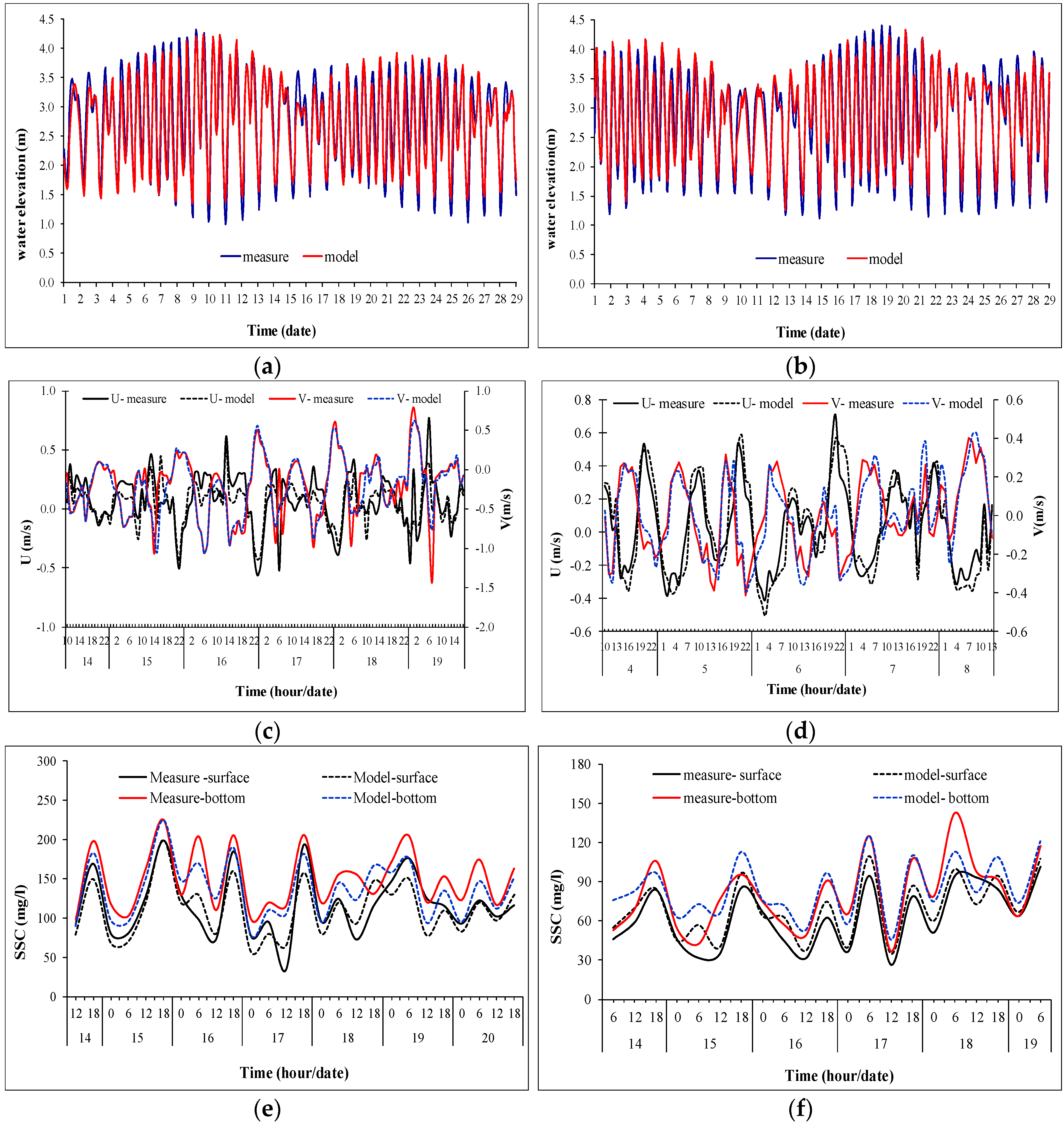
2.3.3. Calibration and Validation Process

Model calibration and validation were conducted simulating low flow and flood seasons of 2012, flood of 2013 and low flow season 2014. The discrepancy between results and measurements was quantified, for each simulation, using the Nash-Sutcliffe efficiency number E [77], calculated as follows:

$$E=1-\frac{\sum {\left(obs-calc\right)}^2}{\sum {\left(obs-mean\right)}^2}$$

(1)

in which the sum of the absolute squared differences between the predicted and observed values is normalized by the variance of the observed values during the period under investigation. E varies from 1.0 (perfect fit) to −∞, a negative value indicating that the mean value of the observed time series would have been a better predictor than the model [78].

2.3.4. Scenario Simulation

In order to describe characteristics of sediment transport in the MRD coastal area, scenarios were set up with different conditions of wave, wind and river discharge. Initial conditions of the scenarios result from a previous simulation (either August for flood season or March for low flow season). At the river boundaries, temperature was fixed at 27.5 °C in the low flow season and at 27.2 °C in the flood season, and salinity was fixed to 0 (there is no income of seawater at the upstream boundaries). The average temperatures do not differ considerably since the low flow season includes both hot months (April to August) and cool months (December, January). The resulting average value is close to the water temperature in the flood season (September, October and November). Temperature and salinity at the open sea boundaries vary from one scenario to another following the climatology.

The average values of river discharge and SSC measured at Can Tho and My Thuan stations during the period 2007–2014 were imposed as boundary conditions. Two groups of scenarios were then considered, referred to as md (low flow season, mostly dry) and mf (flood season):

• during the low flow season (from December to August), the average water river discharges of 3054 m³·s⁻¹ at My Thuan in the Tien River, 3739 m³·s⁻¹ at Can Tho in the Hau River, 52.5 m³·s⁻¹ in the Vamco River and 546.9 m³·s⁻¹ in the Soai Rap River were imposed, with SSC = 50 mg·L⁻¹ at Can Tho, 53.6 mg·L⁻¹ at My Thuan, 55 mg·L⁻¹ in the Vamco and Soai Rap rivers (

  Table 1. Scenario simulations in the low flow season (December to August).

  Scenario	Wave Direction	Duration (Days)	Wave		Wind Velocity (m·s−1)
  			Hs (m)	Tp (s)
  md0		29.87
  md1	NE	0.27	0.5	6.5	4.5
  md2		5.48	2	8.5	7.5
  md3		1.10	4	10.5	10.5
  md4	E	1.64	0.5	6.5	4.5
  md5		23.29	2	8.5	8
  md6		11.78	4	10.5	12.5
  md7		4.38	6	11.5	14.5
  md8		0.55	8	12.5	16.5
  md9	SE	1.64	0.5	6.5	4.5
  md10		18.36	2	8.5	7.5
  md11		9.59	4	10.5	10.5
  md12		3.29	6	11.5	12.5
  md13		0.27	8	12.5	14.5
  md14	S	2.47	0.5	6.5	4.5
  md15		25.21	2	8.5	6.5
  md16		14.80	4	10.5	9.5
  md17		7.67	6	11.5	12.5
  md18		1.10	8	12.5	14.5
  md19	SW	3.29	0.5	6.5	4.5
  md20		45.76	2	8.5	7.5
  md21		31.51	4	10.5	10.5
  md22		21.65	6	11.5	12.5
  md23		6.30	8	12.5	14.5
  md24		2.74	10.5	13.5	16.5

  );
• during the flood season (from September to November), the average water river discharges of 12,530 m³·s⁻¹ at My Thuan, 13,130 m³·s⁻¹ at Can Tho, 177.8 m³·s⁻¹ in the Vamco River and 1310 m³·s⁻¹ in the Soai Rap River were considered, with SSC = 67.8 mg·L⁻¹ at Can Tho, 86.5 mg·L⁻¹ at My Thuan and 70 mg·L⁻¹ at Vamco and Soai Rap (

  Table 2. Scenario simulations in the flood season (September to November).

  Scenario	Wave Direction	Duration (Days)	Wave		Wind Velocity (m·s−1)
  			Hs (m)	Tp (s)
  mf0		13.01
  mf1	NE	0.09	0.5	6.5	4.5
  mf2		2.82	2	9	7.5
  mf3		0.55	4	10.5	9.5
  mf4		0.09	6	11.5	12.5
  mf5	E	0.46	0.5	6.5	4.5
  mf6		7.74	2	9	7.5
  mf7		4.64	4	10.5	10.5
  mf8		2.00	6	11.5	12.5
  mf9		0.09	8	12.5	14.5
  mf10	SE	0.09	0.5	6.5	4.5
  mf11		6.19	2	9	7.5
  mf12		4.55	4	10.5	11
  mf13		1.00	6	11.5	12.5
  mf14	S	0.18	0.5	6.5	4.5
  mf15		7.46	2	9	7.5
  mf16		5.92	4	10.5	11.5
  mf17		2.09	6	11.5	13
  mf18		0.46	8	12.5	15
  mf19	SW	0.27	0.5	6.5	4.5
  mf20		12.56	2	9	7.5
  mf21		11.01	4	10.5	11.5
  mf22		6.28	6	11.5	13
  mf23		1.18	8	12.5	15
  mf24		0.27	10.5	13.5	17

  ).

The variation in SSC values at My Thuan and Can Tho between low flow and flood seasons is not large since these values are constrained by erosion, transport, deposition all along the Mekong River, and by storage and release by the Tonle Sap. However, the seasonal variations of suspended sediment discharge are higher than the seasonal variations of the flow.

The wave and wind conditions were derived from the wave climate obtained over the 22-year period of 1992–2013 by the BMT ARGOSS [49]. For each class of wave direction (NE, E, SE, S, SW) and significant wave height (0.5–1 m, 1–3 m, 3–5 m, 5–7 m, above 7 m), the average durations during the 274 days of the low flow season (from December to August) and the 91 days of the flood season (from September to November) were defined. Adding periods of calm weather (i.e., with significant wave height <0.5 m), we obtained 25 typical scenarios for the low flow season (Table 1) and 25 typical scenarios for the flood season (Table 2). For each scenario, significant wave heights H_s representative of the above described classes were defined as: 0.5 m, 2 m, 4 m, 6 m, 8 m, respectively. Wave peak periods T_p were determined from statistics established over 20 years of measurements, available online at the BMT group website. In each scenario, we assumed that wind was coming from the same direction as the waves, which is mostly the case since the gauging station is located offshore.

Each of the above-defined scenarios was run for a 14.75-day period corresponding to one full neap-spring tide cycle [79]. Each simulation considered real tidal boundary conditions from one typical cycle, which was chosen as the period 11–25 September, 2012.

3. Results

3.1. Model Validation from Field Measurements

Water elevation at hydrometeorological stations of Vung Tau, Binh Dai, An Thuan and Ben Trai (e.g., Figure 2a,b) was used to calibrate (e.g., for the choice of the Manning coefficient) and then validate the model. After calibration, comparisons show good agreement between model results and measurements with E coefficients between 0.68 and 0.85. Current velocity measured in LT1 (Figure 2c), LT2 (Figure 2d), LT3 and LT4 in September 2013 and April 2014 were analyzed to provide horizontal velocity components U and V, which were compared with model simulations. The comparison showed an acceptable agreement between model and measurements with E coefficients between 0.65 and 0.89. Comparisons between measured SSC in LT1 (Figure 2e), LT2 (Figure 2f), LT3, LT4 and modeled SSC also resulted in acceptable E coefficients in the range 0.66–0.78.

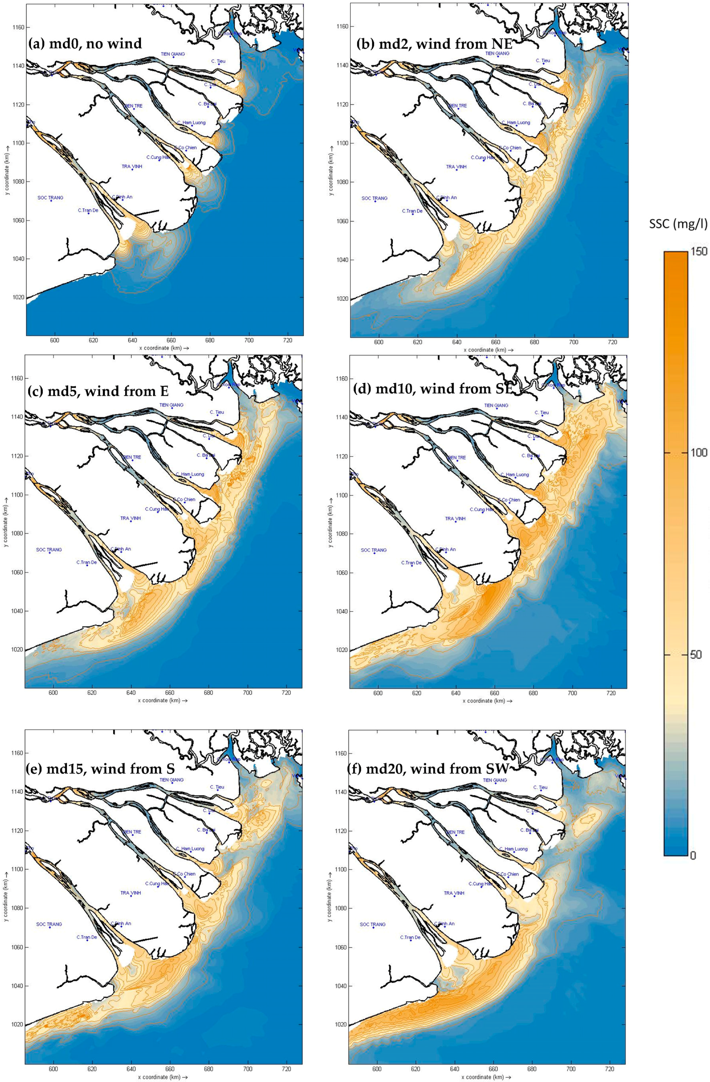
3.2. Spatial Distribution of SSC with or without Waves

Figure 3 (in low flow season) and Figure 4 (in flood season) show the distribution of SSC below the surface in the absence of wind and waves (Figure 3a and Figure 4a), and with waves of significant height of 2 m, coming from 5 different directions from NE to SW. These distributions are provided in Figure 3 and Figure 4 one hour before low tide, which correspond to the maximum extent of the plume to the ocean.

3.2.1. Without Waves

It appears from the wave climate [49] that calm weather conditions (without wave) in the MRD coastal area occurs about 25.2% of the year (14.3% during the flood season and 10.9% during the low flow season). Therefore, annually, there are about 43 days without waves (13 days in flood season and 30 days in the low flow season; see Table 1 and Table 2).

In this case with no waves, the distribution of suspended sediment concentration derives from the interaction between sediments originating from the river and tidal oscillation. In the low flow season, sediments from the river settle in the estuary or very close to the mouths (not further than 10–15 km seawards from the estuaries) with SSC in the range 40–60 mg·L⁻¹ (Figure 3a). There are relevant differences amongst SSC values along the delta: SSC is higher in Southwestern estuaries (Tran De, Dinh An mouths) than in Northeastern estuaries (Tieu, Dai, Ham Luong mouths). In the flood season, SSC varies between 40 and 80 mg·L⁻¹, with higher values in the Southwestern estuaries and river mouth area as well (Figure 4a).

3.2.2. With Waves

With increasing wave height, the combination of waves and tides strengthens resuspension over increasing depths along the delta. As a result, SSC values increase locally and high SSCs also extend further offshore. However, their distribution strongly depends on wave height and direction.

Low flow season. In the low flow season, NE waves extend the plume up to around 15 km from the coast with SSC values of 30–50 mg·L⁻¹ inside and <10 mg·L⁻¹ further offshore with the md2 scenario (Figure 3b). Higher SSC values due to erosion are observed with higher waves (md3 scenario), but the plume pattern remains the same (and its time evolution during the tidal cycle—not shown in this paper—is very similar as well). In the case of waves coming from the East, the turbid plume is slightly less extended offshore than with NE waves but with sensitively higher SSC values (scenario md5, SSC about 40–60 mg·L⁻¹, Figure 3c). SSC values and the plume extent increase with increasing wave height (scenarios md6-md8). Waves from SE have the highest impact on suspended sediment transport because they travel perpendicularly toward the coast. With wave height in the 1–3 m range (scenario md10, Figure 3d), higher SSC values (40–70 mg·L⁻¹) covered the all coastal zones up to 15–20 km from the coast. Outside of 20 km from the coast, SSC decreases to below 20 mg·L⁻¹. Waves from the South have a higher impact on Southwestern estuaries (Dinh An, Tran De, Cung Hau) which experienced higher SSC values (30–50 mg·L⁻¹) than on the Northeastern estuaries (with SSC values in the range 20–40 mg·L⁻¹) (scenario md15, Figure 3e). This trend remains the same with higher waves. Waves from the SW direction cause strong erosion in the southern part of the delta, near Tran De and Dinh An mouths. As a result, SSC is higher (about 60–120 mg·L⁻¹) in the Southwestern part than in the Northeastern coastal area with values almost below 30 mg·L⁻¹ (scenario md20, Figure 3f).

Flood season. During the flood season, mean water river discharge increased about 4 times compared to the low flow season, and SSC in the river increased by 30%–60%. The general patterns of the turbid plume are similar to the ones observed in the low flow season, with almost the same shape and horizontal extension, but with higher SSC values. With waves from the NE, the highest SSC values reach 70–100 mg·L⁻¹ in the Southwestern estuaries (scenario mf2, Figure 4b). With waves from the East, the sediment distribution is quite similar but exhibits slightly higher SSC values around the Northeastern mouths (scenario mf6, Figure 4c). Waves from SE have the higher impact on resuspension and SSC values range from 80 and 150 mg·L⁻¹ all along the delta (scenario mf11, Figure 4d). Waves from the South and the SW induce higher SSC values in the Southwestern estuaries up to 80–120 mg·L⁻¹ (scenario mf15, Figure 4e). High SSC values (80–100 mg·L⁻¹) are also observed around the Southwestern delta when waves originate from the SW, with lower values in the Northern coastal zone (scenario mf20, Figure 4f). Surprisingly, the impact of waves from the SW seems strongly reduced by fresh water flux in the flood season, through the interaction of waves and fresh water (see Figure 3f and Figure 4f). We observed one noticeable difference between the low flow and flood seasons: except for waves from the SE, the highest values of SSC were observed in the Southern estuaries in the case of SW waves in the low flow season (Figure 3f) and in the case of Southern waves in the flood season (Figure 4e).

Globally, the river plume is very narrow and its extent is reduced throughout the year (as also shown by Loisel et al. [25]) for two reasons: (1) most of the particles carried by the river settle in the lower estuary or around the river mouths; (2) the plume is constrained along a baroclinic coastal current as demonstrated by Hordoir et al. [33]. Differences between low flow and flood seasons are small because the turbidity patterns are driven by wave action, more than by the river flow.

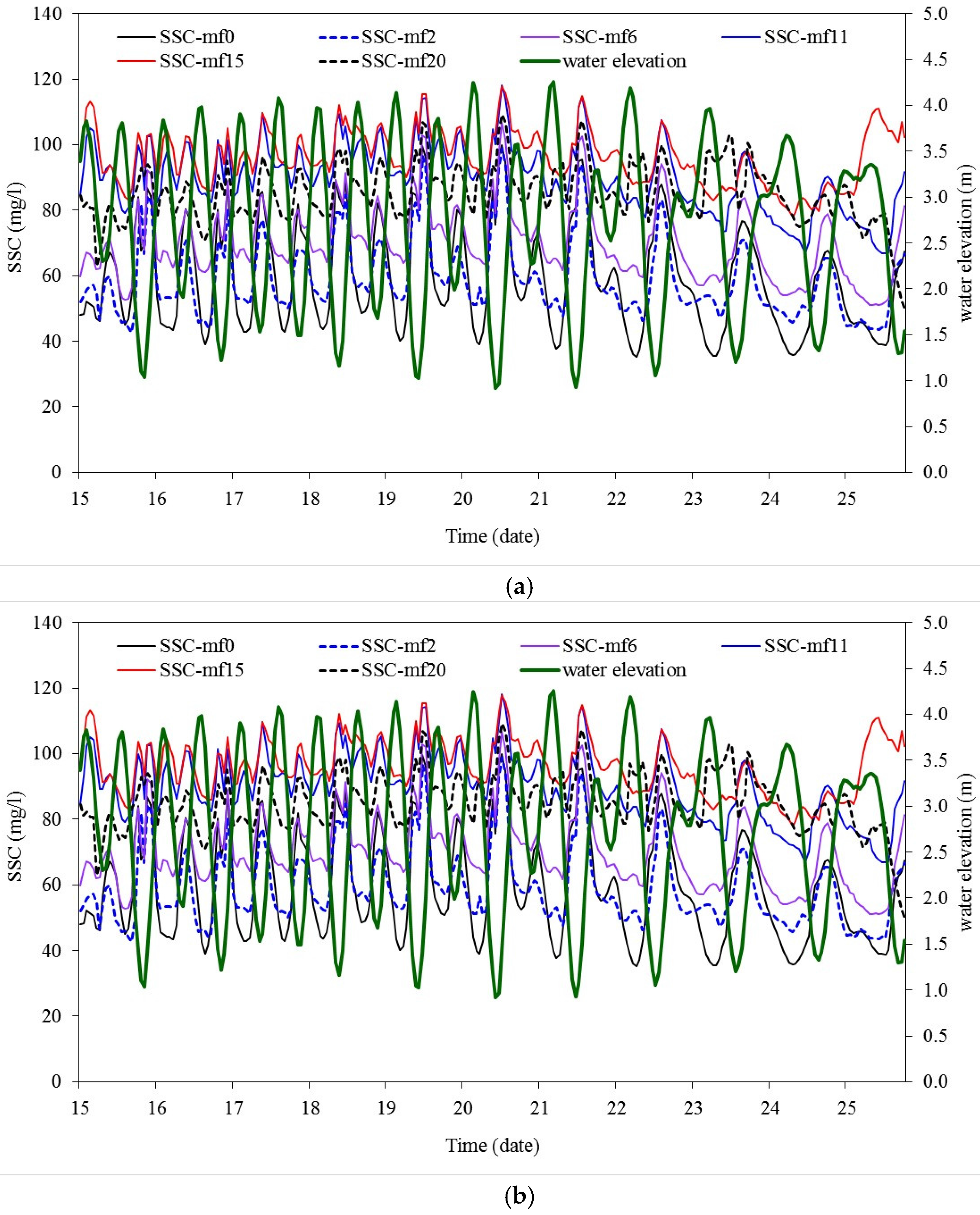
3.3. Temporal Variation of SSC

For a given river discharge, temporal variation of SSC in the MRD coastal area depends on tidal oscillation and wave conditions. Figure 5 shows the water elevation and SSC values at two stations during 11 days over 14.75 of the full spring-neap tide cycle (for readability purpose). The highest SSC values are observed at low tide or at the beginning of the flood. The lowest SSC values are seen 2–3 h after the high tide, during the ebb period (Figure 5). SSC values are also higher during the spring tide (days 18–22) than the neap tide (day 23 and after), but the difference is quite small: less than 10 mg·L⁻¹ at the Northeastern coastal station (Figure 5a), and less than 20 mg·L⁻¹ at the Southwestern coastal station (Figure 5b).

The temporal variation in SSC is similar with or without waves, but SSC values are much higher with waves. In the Northeastern coastal zone, waves from E and SE directions (scenarios mf6 and mf11) induce SSC values 3–4 times higher than under calm conditions, and higher than any other wave direction (Figure 5a). In the Southwestern coastal zone, the highest SSC values occur when waves originate from the S and SW (scenarios mf15 and mf20), 20%–50% higher than when waves come from other directions (Figure 5b).

3.4. Alongshore Sediment Transport

3.4.1. Without Waves

Under calm conditions, a net sediment transport occurs from NE to SW in the low flow season with fluxes across sections m3, m2 and m1 of 0.15, 0.65 and 2.32 × 10³ tons, respectively, during a spring-neap tide cycle (

Table 3. Total sediment flux (10³ tons) transported across the sections under the 50 scenarios. (Positive values represent sediment transport from the SW to NE, negative values from the NE to SW).

Low Flow Season					Flood Season
Scenario	Wave Direction	Cross Section			Scenario	Wave Direction	Cross Section
		m1	m2	m3			m1	m2	m3
md0		−2.32	−0.65	−0.15	mf0		−5.04	−0.37	0.71
md1	NE	−0.05	−0.02	−0.01	mf1	NE	−0.07	−0.01	0.00
md2		−7.02	−4.44	−1.52	mf2		−7.28	−3.04	−0.89
md3		−6.38	−4.43	−1.23	mf3		−3.65	−2.19	−0.49
md4	E	−0.30	−0.10	−0.06	mf4		−1.50	−1.00	−0.21
md5		−39.60	−15.97	−5.49	mf5	E	−0.31	−0.04	0.01
md6		−117.58	−51.71	−5.98	mf6		−21.38	−6.11	−1.54
md7		−81.66	−37.03	−3.30	mf7		−38.83	−15.98	−1.35
md8		−16.91	−7.61	−0.80	mf8		−29.81	−13.39	0.26
md9	SE	−0.39	−0.07	−0.07	mf9		−0.02	−1.08	0.02
md10		−24.16	2.63	11.12	mf10	SE	−0.08	0.00	0.00
md11		−53.18	17.96	37.14	mf11		−19.14	1.47	6.24
md12		−36.69	15.49	26.06	mf12		−41.88	13.45	27.64
md13		−5.53	2.12	3.23	mf13		−15.00	5.97	10.29
md14	S	−0.23	0.02	0.01	mf14	S	−0.07	0.01	0.02
md15		2.02	9.39	3.83	mf15		1.89	0.29	3.79
md16		30.21	47.87	32.25	mf16		38.13	6.13	41.94
md17		62.96	80.14	67.92	mf17		23.29	22.69	25.24
md18		38.93	44.46	36.71	mf18		10.61	12.48	9.27
md19	SW	−0.13	0.02	0.05	mf19	SW	−0.06	0.01	0.03
md20		67.09	23.05	6.33	mf20		10.42	6.02	2.51
md21		229.37	125.38	51.66	mf21		85.28	55.33	19.94
md22		361.55	201.51	95.72	mf22		95.57	58.32	21.96
md23		234.97	128.43	63.25	mf23		37.57	20.87	8.62
md24		187.43	104.88	54.69	mf24		15.46	8.40	3.65

). In the flood season, with a much higher river discharge, the sediment flux to the Southwest across the Southern transect m1 more than doubled (5.04 × 10³ tons) as compared to the low flow season, the sediment flux across section m2 decreased by about 40%, and a flux of 0.71 × 10³ tons was generated towards the Northeastern direction across section m3 directly North to the Northern mouths (Table 3).

3.4.2. Sensitivity to Wave Height and Direction

Low flow season. Waves from the NE cause a net alongshore sediment transport to the SW (Table 3). This flux increases over each cross section from the Northern estuaries to the Southern ones, with net transports of 2.76 × 10³ tons across m3, 8.89 across m2 and 13.45 across m1 (

Table 4. Total sediment flux (10³ tons) transported across sections per year. (Positive values represent sediment transport from the SW to NE, negative values from the NE to SW).

Wave Direction	Low Flow Season			Flood Season			Total Year
	Cross Section			Cross Section			Cross Section
	m1	m2	m3	m1	m2	m3	m1	m2	m3
calm	−2.32	−0.65	−0.15	−5.04	−0.37	0.71	−7.356	−1.013	0.555
NE	−13.45	−8.89	−2.76	−12.51	−6.24	−1.59	−25.95	−15.12	−4.35
E	−256.06	−112.43	−15.64	−90.35	−36.59	−2.59	−346.41	−149.02	−18.24
SE	−119.95	38.13	77.48	−76.11	20.90	44.18	−196.06	59.03	121.66
S	133.88	181.88	140.72	73.84	41.61	80.26	207.73	223.49	220.98
SW	1080.28	583.25	271.69	244.25	148.95	56.70	1324.53	732.20	328.39
NEward	1214.52	803.34	489.96	318.22	211.45	182.13	1532.26	1014.72	671.59
SWward	−392.13	−122.03	−18.62	−184.14	−43.20	−4.47	−575.78	−165.15	−22.58
Net transport	822.39	681.31	471.34	134.08	168.25	177.66	956.48	849.57	649.01

). They are mainly due to waves higher than 2 m (scenarios md2 and md3, Table 3). Waves from the East globally induce a higher sediment flux Southwestward, which also increases from across section m3 (15.6 × 10³ tons), to m2 (112 × 10³ tons) and m1 (256 × 10³ tons). These fluxes are higher than with NE waves by a factor of 20 in m1, 12 in m2 and 5 in m3 (Table 4). In the low flow season, with waves from the SE (i.e., perpendicular to the coastline), the alongshore sediment transport is globally oriented to the NE direction in the Northern and central area (m3 and m2), and to the SW in the Southern area (1). The global flux to the SW across m1 is much lower than when waves come from the East (120 × 10³ tons instead of 256 × 10³ tons, see Table 4). Waves coming from the S or SW globally induce alongshore sediment fluxes in a Northwestward direction. When waves come from the South, the flux is higher in the central zone (m2, 182 × 10³ tons), while it is higher in the South (m1, 1080 × 10³ tons) in the case of SW waves. The highest values of sediment flux occur when waves come from SW, with decreasing fluxes from the Southwest to the Northeastern area (1080 × 10³ tons across m1, 583 across m2 and 272 across m3). A total of 89% of the total flux of sediment across m1 section is due to SW waves. This percentage drops to 73% and 55% across sections m2 and m3, respectively.

Flood season. Although the river discharge is much higher than in the low flow season, the alongshore sediment transport qualitatively occurs in the same way in both seasons. In the case of waves from the NE, the net alongshore sediment transport is still oriented to the Southwest, with increasing values from the North to the South: 1.59 × 10³ tons across m3, 6.24 × 10³ tons across m2, and 12.51 × 10³ tons across m1 (Table 4). When waves come from the East, sediment is mainly transported alongshore to the SW, with increasing values from m3 to m1. However, we observe that the net transport is oriented Northeastward at m3 (in the North) in case of wave height less than 2.0 m or higher than 4.0 m (Table 3). Similar to the low flow season, waves from the SE induce alongshore sediment transport Northeastward in the Northern (m3) and central delta (m2), and Southwestward in the South (m1) in the flood season. The highest flux occurs across section m1 from the NE to SW with about 76 × 10³ tons (Table 4). With waves from the South, the net alongshore sediment transport is significantly higher in the Northeast (80 × 10³ tons across m3, see Table 4) and Southwest (74 × 10³ tons across m1) than in the middle delta (42 × 10³ tons across m2). Sediment transport is oriented to the NE, except across section m1 with waves less than 0.5 m (Table 3). The same behavior is observed in the case of waves from the SW, with decreasing flux from the South to the North: ~244 × 10³ tons (m1), 146 × 10³ tons (m2) and 57 × 10³ tons (m3). In the Southwestern estuaries of Dinh An-Tran De, the net sediment transport is oriented Southwestward in the case of small waves, and Northeastward with waves higher than 0.5 m (Table 3). In that case, the net alongshore sediment flux is thus a consequence of resuspension of sediment along the Southern delta, along the Ca Mau peninsula.

Globally, the net alongshore sediment transport is oriented to the Northeast of the MRD coastal area in both seasons (Table 4). In the MRD coastal area, the flood season lasts about 3 months. Even if the instantaneous sediment discharge is much higher, the net alongshore sediment transport is much higher in the low flow season than in the flood season: 86% of the net annual alongshore transport across m1 occurs in the low flow season (822 × 10³ tons vs. 134, see Table 4), 80% across m2 and 73% across m3. Much of the sediment brought by the river settle and is deposited in the estuaries and close to the river mouths.

In the Southwestern area (across section m1), the annual alongshore sediment transport to the Northeast (1532 × 10³ tons, Table 4) is due to the waves coming from the S and SW and thus to resuspension along the Ca Mau peninsula. Waves from the NE, E and SE, as well as calm conditions, induce a sediment transport of about 575 × 10³ tons to the Southwest.

In the middle coastal part (across section m2 between the Tien River mouth and Hau River mouth), waves from the SE, S and SW generate an annual sediment transport to the Northeast of 1014 × 10³ tons, while calm conditions and waves from the NE and E generate alongshore transport of 165 × 10³ tons.

In the Northern coastal part (across section m3), the total flux to the Northeast of 672 × 10³ tons is generated in the case of waves from the SE, S and SW, while the sediment transport to the Southwest (in case of waves from NE and E) is restricted to about 23 × 10³ tons.

As the net alongshore sediment transport decreases from the Southwest (m1) to the Northeast (m3), it shows that the source of global alongshore sediment transport along the MRD is double, generated both by the sediments settling from the river plume, and by erosion, which seems to occur mainly along the Ca Mau peninsula to the Southwest, while a net deposition occurs to the North of section m1.

4. Discussion and Conclusions

In this study, the cumulative alongshore transport of suspended sediments across three sections was estimated to be less than 1.5 × 10⁶ tons per year in a given direction. A comment is necessary since the average sediment load of the Mekong River was estimated to be around 145 × 10⁶ t yr⁻¹ over the last 3 k yr [32,39]. In fact, using a detailed numerical model of sediment transport, erosion and deposition within the Mekong delta, Manh et al. [23] reported that total sediment load to the coast was about 50%–60% of the sediment flux at the gauging station of Kratie in Cambodia during a year of low flow (like 2010) or normal condition (like 2009), and that this percentage was about 48% during a year with extreme flooding (like in 2011). In a normal flood year, they estimated that the sediment load to the coast was about 42 × 10⁶ tons per year [23]. A complementary study by Xue et al. [24] reported that 86.9% of the sediment coming from the Mekong River system was trapped in the MRD estuaries and nearshore area. As a result, in normal years, around 5.5 × 10⁶ tons of sediments are transported alongshore and seaward. As most of these sediments seem to settle and deposit very near to the mouths, the estimations obtained for the cumulated alongshore transports in this study are thus consistent with previous studies.

The present study underlined the role of waves in the sediment redistribution along the delta. Under the present configuration and shoreline, the main alongshore flux is not due to the fate of the river plume but to the action of waves coming from the SW and S, which induce resuspension along the Southern delta and sediment transport to the Northeast. Under small wave conditions, the highest SSC values are seen in the estuaries or very close to the mouths. With increasing wave height, SSC values increase and zones with high SSC values extend a little bit offshore. However, the plume never extends further than 20 km from the coast, which is the limit of the subaqueous delta. Our results are consistent with those from Hordoir et al. [33], who showed that the plume of the Mekong River is dominated by geostrophy from a dynamical perspective, with freshwater advected by a coastally trapped baroclinic current. This behavior was confirmed by a Rossby number less than 1 throughout the year, due to the large freshwater discharge.

Waves from the SW direction (and to a lesser extent waves from the South) are mainly responsible of the net alongshore transport to the Northeast of the delta. Waves from the SW generate about 86% of the Northeastward flux in the Southern delta (1324 × 10³ tons over 1532 across section m1), 72% along the central delta (m2) and 49% in the Northern part (across m3).

A companion paper [80] provided the maps of deposition and erosion (in mm) in the study area, per season, and per year. It showed that: (1) deposition occurs in the lower estuary at a rate reaching 40–50 mm yr⁻¹; (2) deposition is decreasing fast with decreasing water depth in front of the mouths up to 5 m depth; (3) patches of erosion are found along the MRD in water between 5 and 10 m depth; (4) further offshore at 10–15 m depths, deposition occurs at rates <10 mm yr⁻¹. These values are consistent with the accumulation rates determined by Ta et al. [32] in front of the MRD for the most recent period. Erosion zones and rates differ slightly from these given by Xue et al. [25] over water depth between 5 and 10 m since their study did not take into account the action of the highest waves.

The net sediment transport to the Northeast observed in the Southern part of the delta (along Ca Mau cape) is the main original result of our calculations. This trend is consistent with simulations of the Mekong shelf circulation and sediment transport and dispersal performed for 2005 by Xue et al. [22], who reported that the Southwestern part of the MRD (between Tran De mouth and Ca Mau Cape) receives very few sediments from the Mekong River. Deposition in that area should almost result from a slow but persistent deposition process occurring over a much longer (millennial) time scale. Regardless, the sediment deficit along the Southern coastal area of the delta, which results mainly from the action of waves coming from the S and SW in low flow season, is consistent with the geological studies and with the severe erosion along the Ca Mau peninsula, estimated to be an average of 1.1 km² yr⁻¹ since 1885 [81].

Remote sensing data can be used in complement to numerical simulations to study the river plume dynamics and sediment transport [82,83,84,85,86]. Satellite data are available under clear sky conditions only; such data are numerous during the dry season but less abundant during the wet and mostly cloudy season, which makes it difficult to estimate sediment budgets from remote sensing alone. Continuous and costly measurements or modeling (after validation from in situ data) are the two ways to estimate annual fluxes such as given in this study (Table 4). However, such estimates could greatly benefit from the available remote sensing data (e.g., [25]) to offer a synoptic view to complement local measurements and further constraint the model. Such a coupling between modeling, satellite data analysis and field measurements may be envisaged in a future step over the Mekong coastal zone.

References

1. Liu, J.P.; Xue, Z.; Ross, K.; Wang, H.J.; Yang, Z.S.; Li, A.C.; Gao, S. Fate of sediments delivered to the sea by Asian large rivers: Long-distance transport and formation of remote alongshore clinothems. Sediment. Rec. 2009, 7, 4–9. [Google Scholar]
2. Saito, Y.; Chaimanee, N.; Jarupongsakul, T.; Syvitski, J.P.M. Shrinking megadeltas in Asia: Sea-level rise and sediment reduction impacts from case study of the Chao Phraya delta. Newsl. IGBP/IHDP Land Ocean Interact. Coast. Zone 2007, 2, 3–9. [Google Scholar]
3. Vörösmarty, C.J.; Meybeck, M.; Fekete, B.; Sharma, K.; Green, P.; Syvitski, J.P.M. Anthropogenic sediment retention: Major global impact from registered river impoundments. Glob. Planet. Chang. 2003, 39, 169–190. [Google Scholar] [CrossRef]
4. Syvitski, J.P.M.; Saito, Y. Morphodynamics of Deltas under the Influence of Humans. Glob. Planet. Chang. 2007, 57, 261–282. [Google Scholar] [CrossRef]
5. Wang, H.J.; Yang, Z.S.; Saito, Y.; Liu, J.P.; Sun, X. Interannual and seasonal variation of the Huanghe (Yellow River) water discharge over the past 50 years: Connections to impacts from ENSO events and dams. Glob. Planet. Chang. 2006, 50, 212–225. [Google Scholar] [CrossRef]
6. Wang, H.J.; Yang, Z.S.; Wang, Y.; Saito, Y.; Liu, J.P. Reconstruction of sediment flux from the Changjiang (Yangtze River) to the sea since the 1860s. J. Hydrol. 2008, 349, 318–332. [Google Scholar] [CrossRef]
7. Vinh, V.D.; Ouillon, S.; Tanh, T.D.; Chu, L.V. Impact of the Hoa Binh dam (Vietnam) on water and sediment budgets in the Red River basin and delta. Hydrol. Earth Syst. Sci. 2014, 18, 3987–4005. [Google Scholar] [CrossRef]
8. Schlünz, B.; Schneider, R.R. Transport of terrestrial organic carbon to the oceans by rivers: Re-estimating flux- and burial rates. Int. J. Earth Sci. 2000, 88, 599–606. [Google Scholar] [CrossRef]
9. Viers, J.; Dupré, B.; Gaillardet, J. Chemical composition of suspended sediments in World Rivers: New insights from a new database. Sci. Total Environ. 2009, 407, 853–868. [Google Scholar] [CrossRef] [PubMed]
10. Rochelle-Newall, E.J.; Chu, V.T.; Pringault, O.; Amouroux, D.; Arfi, R.; Bettarel, Y.; Bouvier, T.; Bouvier, C.; Got, P.; Nguyen, T.M.; et al. Phytoplankton diversity and productivity in a highly turbid, tropical coastal system (Bach Dang Estuary, Vietnam). Mar. Pollut. Bull. 2011, 62, 2317–2329. [Google Scholar] [CrossRef] [PubMed]
11. Mari, X.; Torréton, J.P.; Chu, V.T.; Lefebvre, J.P.; Ouillon, S. Seasonal aggregation dynamics along a salinity gradient in the Bach Dang estuary, North Vietnam. Estuar. Coast. Shelf Sci. 2012, 96, 151–158. [Google Scholar] [CrossRef]
12. Navarro, P.; Amouroux, D.; Duong, T.N.; Rochelle-Newall, E.; Ouillon, S.; Arfi, R.; Chu, V.T.; Mari, X.; Torréton, J.P. Butyltin and mercury compounds fate and tidal transport in waters of the tropical Bach Dang estuary (Haiphong, Vietnam). Mar. Pollut. Bull. 2012, 64, 1789–1798. [Google Scholar] [CrossRef] [PubMed]
13. Syvitski, J.P.M.; Vörösmarty, C.J.; Kettner, A.J.; Green, P. Impact of Humans on the Flux of Terrestrial Sediment to the Global Coastal Ocean. Science 2005, 308, 376. [Google Scholar] [CrossRef] [PubMed]
14. Ouillon, S. Erosion and sediment transport: Width and stakes. Houille Blanche 1998, 53, 52–58. [Google Scholar] [CrossRef]
15. Clift, P.D.; Plumb, R.A. The Asian Monsoon: Causes, History and Effects; Cambridge University Press: Cambridge, UK, 2008; p. 288. [Google Scholar] [CrossRef]
16. Tamura, T.; Horaguchi, K.; Saito, Y.; Nguyen, V.L.; Tateishi, M.; Ta, T.K.O.; Nanayama, F.; Watanabe, K. Monsoon-influenced variations in morphology and sediment of a mesotidal beach on the Mekong River Delta coast. Geomorphology 2010, 116, 11–23. [Google Scholar] [CrossRef]
17. Eastham, J.; Mpelasoka, F.; Mainuddin, M.; Ticehurst, C.; Dyce, P.; Hodgson, G.; Ali, R.; Kirby, M. Mekong River Basin Water Resources Assessment: Impacts of Climate Change; CSIRO National Research Flagship, Water for a Healthy Country: Canberra, Australia, 2008. [Google Scholar]
18. Nguyen, V.L.; Ta, T.K.O.; Tateishi, M. Late Holocene depositional environments and coastal evolution of the Mekong River Delta, Southern Vietnam. J. Asian Earth Sci. 2000, 18, 427–439. [Google Scholar] [CrossRef]
19. Walling, D.E. The changing sediment load of the Mekong River. AMBIO 2008, 37, 150–157. [Google Scholar] [CrossRef]
20. Xue, Z.; Liu, J.P.; Ge, Q. Changes in hydrology and sediment delivery of the Mekong River in the last 50 years: Connection to damming, monsoon, and ENSO. Earth Surf. Process. Landf. 2011, 36, 296–308. [Google Scholar] [CrossRef]
21. Le, T.V.H.; Nguyen, H.N.; Wolanski, E.; Tran, T.C.; Haruyama, S. The combined impact on the flooding in Vietnam’s Mekong River Delta of local man-made structures, sea level rise, and dams upstream in the river catchment. Estuar. Coast. Shelf Sci. 2007, 71, 110–116. [Google Scholar] [CrossRef]
22. Wang, J.J.; Lu, X.X.; Kummu, M. Sediment load estimates and variations in the lower Mekong River. River Res. Appl. 2011, 27, 33–46. [Google Scholar] [CrossRef]
23. Manh, N.V.; Dung, N.V.; Hung, N.N.; Merz, B.; Apel, H. Large-scale suspended sediment transport and sediment deposition in the Mekong delta. Hydrol. Earth Syst. Sci. 2014, 18, 3033–3053. [Google Scholar] [CrossRef] [Green Version]
24. Xue, Z.; He, R.; Liu, J.P.; Warner, J.C. Modeling transport and deposition of the Mekong River sediment. Cont. Shelf Res. 2012, 37, 66–78. [Google Scholar] [CrossRef]
25. Loisel, H.; Mangin, A.; Vantrepotte, V.; Dessailly, D.; Dinh, N.D.; Garnesson, P.; Ouillon, S.; Lefebvre, J.P.; Mériaux, X.; Phan, M.T. Analysis of the suspended particulate matter concentration variability of the coastal waters under the Mekong’s influence: A remote sensing approach. Remote Sens. Environ. 2014, 150, 218–230. [Google Scholar] [CrossRef]
26. Szczuciński, W.; Jagodziński, R.; Hanebuth, T.J.J.; Stattegger, K.; Wetzel, A.; Mitręga, M.; Unverricht, D.; Phach, P.V. Modern sedimentation and sediment dispersal pattern on the continental shelf off the Mekong River delta, South China Sea. Glob. Planet. Chang. 2013, 110, 195–213. [Google Scholar] [CrossRef]
27. Wolanski, E.; Ngoc Huan, N.; Trong Dao, L.; Huu Nhan, N.; Ngoc Thuy, N. Fine sediment dynamics in the Mekong River Estuary, Vietnam. Estuar. Coast. Shelf Sci. 1996, 43, 565–582. [Google Scholar] [CrossRef]
28. Wolanski, E.; Nhan, N.H.; Spagnol, S. Sediment dynamics during low flow conditions in the Mekong River Estuary, Vietnam. J. Coast. Res. 1998, 14, 472–482. [Google Scholar]
29. Hein, H.; Hein, B.; Pohlmann, T. Recent dynamics in the region of Mekong water influence. Glob. Planet. Chang. 2013, 110, 183–194. [Google Scholar] [CrossRef]
30. Mekong River Commission (MRC). State of the Basin Report: 2003; MRC: Phnom Penh, Cambodia, 2003. [Google Scholar]
31. Milliman, J.D.; Meade, R.H. World-wide delivery of river sediment to the oceans. J. Hydrol. 1983, 91, 1–21. [Google Scholar] [CrossRef]
32. Ta, K.T.O.; Nguyen, V.L.; Tateishio, M.; Kobayashi, I.; Tanabe, S.; Saito, Y. Holocene delta evolution and sediment discharge of the Mekong River, southern Vietnam. Quat. Sci. Rev. 2002, 21, 1807–1819. [Google Scholar] [CrossRef]
33. Hordoir, R.; Nguyen, K.D.; Polcher, J. Simulating tropical river plumes, a set of parametrizations based on macroscale data: A test case in the Mekong Delta region. J. Geophys. Res. 2006, 111, C09036. [Google Scholar] [CrossRef]
34. Snidvongs, A.; Teng, S.K. Global International Waters Assessment, Mekong River GIWA Regional Assessment 55; University of Kalmar: Kalmar, Sweden, 2006. [Google Scholar]
35. Unverricht, D.; Szczuciński, W.; Stattegger, K.; Jagodziński, R.; Le, X.T.; Kwong, L.L.W. Modern sedimentation and morphology of the subaqueous Mekong delta, Southern Vietnam. Glob. Planet. Chang. 2013, 110, 223–235. [Google Scholar] [CrossRef]
36. Deltares. Mekong Delta Water Resources Assessment Studies; Report of the Vietnam-Netherlands Mekong Delta Masterplan Project; Deltares: Delft, The Netherlands.
37. Vietnamese National Centre for Hydro-Meteorological Forecasts. Statistics on Typhoon Occurrence in Vietnam. 2016. Available online: http://ttnh.vnea.org (accessed on 20 April 2016).
38. Tri, V.K. Hydrology and hydraulic infrastructure systems in the Mekong delta, Vietnam. In The Mekong Delta System; Renaud, F.G., Kuenzer, C., Eds.; Springer: Dordrecht, Germany, 2012; pp. 49–82. [Google Scholar] [CrossRef]
39. Lu, X.X.; Siew, R.Y. Water discharge and sediment flux changes over the past decades in the Lower Mekong River: Possible impacts of the Chinese dams. Hydrol. Earth Syst. Sci. 2006, 10, 181–195. [Google Scholar] [CrossRef]
40. Kubicki, A. Large and very large subaqueous delta dunes on the continental shelf off southern Vietnam, South China Sea. Geo-Mar. Lett. 2008, 28, 229–238. [Google Scholar] [CrossRef]
41. Nguyen, C.T. Processes and Factors Controlling and Affecting the Retreat of Mangrove Shorelines in South Vietnam. Ph.D. Thesis, Kiel University, Kiel, Germany, 2012. [Google Scholar]
42. Allen, G.P.; Salomon, J.C.; Bassoulet, P.; du Penhoat, Y.; de Grandpre, C. Effects of tides on mixing and suspended sediment transport in macrotidal estuaries. Sediment. Geol. 1980, 26, 69–90. [Google Scholar] [CrossRef]
43. Dyer, K.R. Coastal and Estuarine Sediment Dynamics; Wiley: Chichester, UK, 1986; p. 342. [Google Scholar] [CrossRef]
44. Dronkers, J. Tide-induced residual transport of fine sediment. In Physics of Shallow Estuaries and Bays; van de Kreeke, J., Ed.; Lecture Notes Coastal Estuarine Studies, Volome 16; Springer: Berlin, Germany, 1986; pp. 228–244. [Google Scholar] [CrossRef]
45. Sottolichio, A.; Le Hir, P.; Castaing, P. Modeling mechanisms for the turbidity maximum stability in the Gironde estuary, France. Proc. Mar. Sci. 2001, 3, 373–386. [Google Scholar] [CrossRef]
46. Lefebvre, J.P.; Ouillon, S.; Vinh, V.D.; Arfi, R.; Panche, J.Y.; Mari, X.; Van Thuoc, C.; Torréton, J.P. Seasonal variability of cohesive sediment aggregation in the Bach Dang-Cam Estuary, Haiphong (Vietnam). Geo-Mar. Lett. 2012, 32, 103–121. [Google Scholar] [CrossRef]
47. Weatherall, P.; Marks, K.M.; Jakobsson, M.; Schmitt, T.; Tani, S.; Arndt, J.E.; Rovere, M.; Chayes, D.; Ferrini, V.; Wigley, R. A new digital bathymetric model of the world’s oceans. Earth Space Sci. 2015, 2, 331–345. [Google Scholar] [CrossRef]
48. Lanh, D.T. Integrated Water Resources Management and Sustainable Use for the Dong Nai River System; Technical Report of the Project KC.08.18/06-10; The Southern Institute of Water Resources Research: Ho Chi Minh City, Vietnam, 2010. (In Vietnamese) [Google Scholar]
49. Groenewoud, P. Overview of the Service and Validation of the Database; Reference: RP_A870; BMT ARGOSS: Marknesse, The Netherlands, 2011. [Google Scholar]
50. Lefevre, F.; Lyard, F.; Le Provost, C.; Schrama, E.J.O. FES99: A global tide finite element solution assimilating tide gauge and altimetric information. J. Atmos. Ocean. Technol. 2002, 19, 1345–1356. [Google Scholar] [CrossRef]
51. Lyard, F.; Lefevre, F.; Letellier, T.; Francis, O. Modelling the global ocean tides: Modern insights from FES2004. Ocean Dyn. 2006, 56, 394–415. [Google Scholar] [CrossRef]
52. World Ocean Atlas 2013 Version 2 (WOA13 V2). Available online: https://www.nodc.noaa.gov/OC5/woa13/ (accessed on 20 April 2016).
53. Deltares Systems. Delft3D-FLOW User Manual: Simulation of Multi-Dimensional Hydrodynamic Flows and Transport Phenomena, including Sediments; Technical Report; Deltares: Delft, The Netherlands, 2014. [Google Scholar]
54. Booij, N.; Ris, R.C.; Holthuijsen, L.H. A third-generation wave model for coastal regions: 1. Model description and validation. J. Geophys. Res. 1999, 104, 7649–7666. [Google Scholar] [CrossRef]
55. Ris, R.C.; Holthuijsen, L.H.; Booij, N. A third-generation wave model for coastal regions: 2. Verification. J. Geophys. Res. 1999, 104, 7667–7681. [Google Scholar] [CrossRef]
56. Deltares Systems. Delft3D-WAVE User Manual: Simulation of Short-Crested Waves with SWAN; Technical Report; Deltares: Delft, The Netherlands, 2014. [Google Scholar]
57. Jouon, A.; Lefebvre, J.P.; Douillet, P.; Ouillon, S.; Schmied, L. Wind wave measurements and modelling in a fetch-limited semi-enclosed lagoon. Coast. Eng. 2009, 56, 599–608. [Google Scholar] [CrossRef]
58. Hasselmann, K.; Barnett, T.P.; Bouws, E.; Carlson, H.; Cartwright, D.E.; Enke, K.; Ewing, J.; Gienapp, H.; Hasselmann, D.E.; Kruseman, P.; et al. Measurements of Wind Wave Growth and Swell Decay during the Joint North Sea Wave Project (JONSWAP). Deutsche Hydrographische Zeitschrift 8 (12); Deutsches Hydrographisches Institut: Hamburg, Germany, 1973. [Google Scholar]
59. Bouws, E.; Komen, G. On the balance between growth and dissipation in an extreme, depth-limited wind-sea in the southern North Sea. J. Phys. Oceanogr. 1983, 13, 1653–1658. [Google Scholar] [CrossRef]
60. Battjes, J.; Janssen, J. Energy loss and set-up due to breaking of random waves. In Proceedings of the 16th International Conference Coastal Engineering, ASCE, Hamburg, Germany, 26 August–6 September 1978; pp. 569–587.
61. Arcement, G.J., Jr.; Schneider, V.R. Guide for Selecting Manning’s Roughness Coefficients for Natural Channels and Flood Plains. U.S. Geological Survey Water Supply Paper 2339; 1989. Available online: http://www.fhwa.dot.gov/bridge/wsp2339.pdf (accessed on 20 April 2016). [Google Scholar]
62. Simons, D.B.; Senturk, F. Sediment Transport Technology—Water and Sediment Dynamics; Water Resources Publications: Littleton, CO, USA, 1992. [Google Scholar]
63. Uittenbogaard, R.E. Model for Eddy Diffusivity and Viscosity Related to Sub-Grid Velocity and Bed Topography; Technical Report; WL Delft Hydraulics: Delft, The Netherlands, 1998. [Google Scholar]
64. Van Vossen, B. Horizontal Large Eddy Simulations; Evaluation of Computations with DELFT3D-FLOW; Report MEAH-197; Delft University of Technology: Delft, The Netherlands, 2000. [Google Scholar]
65. Van Rijn, L.C. Unified view of sediment transport by currents and waves, Part II: Suspended transport. J. Hydraul. Eng. 2007, 133, 668–689. [Google Scholar] [CrossRef]
66. Partheniades, E. Erosion and deposition of cohesive soils. J. Hydraul. Div. 1965, 91, 105–139. [Google Scholar]
67. Krone, R.B. Flume Studies of the Transport of Sediment in Estuarial Shoaling Processes; Hydraulic Engineering Laboratory and Sanitary Engineering Research Laboratory, University of California: Berkeley, CA, USA, 1962. [Google Scholar]
68. Douillet, P.; Ouillon, S.; Cordier, E. A numerical model for fine suspended sediment transport in the south-west lagoon of New-Caledonia. Coral Reefs 2001, 20, 361–372. [Google Scholar] [CrossRef]
69. Winterwerp, J.C.; van Kesteren, W.G.M. Introduction to the Physics of Cohesive Sediment in the Marine Environment; Elsevier: Amsterdam, The Netherlands, 2004; pp. 1–466. [Google Scholar]
70. Hung, N.N.; Delgado, J.M.; Güntner, A.; Merz, B.; Bárdossy, A.; Apel, H. Sedimentation in the floodplains of the Mekong Delta, Vietnam Part II: Deposition and erosion. Hydrol. Process. 2004, 28, 3145–3160. [Google Scholar] [CrossRef]
71. Portela, L.I.; Ramos, S.; Rexeira, A.T. Effect of salinity on the settling velocity of fine sediments of a harbour basin. J. Coast. Res. 2013, 2, 1188–1193. [Google Scholar] [CrossRef]
72. Van Rijn, L.C. Mathematical modeling of suspended sediment in non-uniform flows. J. Hydraul. Eng. 1986, 112, 433–455. [Google Scholar] [CrossRef]
73. Ouillon, S.; Le Guennec, B. Modelling non-cohesive suspended sediment transport in 2D vertical free surface flows. J. Hydraul. Res. 1996, 34, 219–236. [Google Scholar] [CrossRef]
74. Van Rijn, L. Principles of Sediment Transport in Rivers, Estuaries and Coastal Seas; Aqua Publications: Amsterdam, The Netherlands, 1993. [Google Scholar]
75. Madsen, O.S. Spectral wave–current bottom boundary layer flows. In Proceedings of the 24th International Conference on Coastal Engineering Research Council, Kobe, Japan, 23–28 October 1994; pp. 384–398. [CrossRef]
76. Walstra, D.J.R.; Roelvink, J.A. 3D Calculation of Wave Driven Cross-shore Currents. In Proceedings of the 27th International Conference on Coastal Engineering, Sydney, Australia, 16–21 July 2000; pp. 1050–1063. [CrossRef]
77. Nash, J.E.; Sutcliffe, J.V. River flow forecasting through conceptual models, Part I—A discussion of principles. J. Hydrol. 1970, 10, 282–290. [Google Scholar] [CrossRef]
78. Krause, P.; Boyle, D.P.; Bäse, F. Comparison of different efficiency criteria for hydrological model assessment. Adv. Geosci. 2005, 5, 89–97. [Google Scholar] [CrossRef]
79. Kvale, E.P.; Archer, A.W.; Johnson, H.R. Daily, monthly, and yearly tidal cycles within laminated siltstones of the Mansfield Formation (Pennsylvanian) of Indiana. Geology 1989, 17, 365–368. [Google Scholar] [CrossRef]
80. Vinh, V.D.; Lan, T.D.; Tu, T.A.; Anh, N.K.; Tien, N.N. Influence of dynamic processes on morphological change in the coastal area of Mekong river mouth. J. Mar. Sci. Technol. 2016, 16, 32–45. [Google Scholar] [CrossRef]
81. Saito, Y. Deltas in Southeast and East Asia: Their evolution and current problems. In APN/SURVAS/LOICZ Joint Conference on Coastal Impact of Climate Change and Adaption in the Asia-Pacific Region; Mimura, N., Yokoki, H., Eds.; APN: Kobe, Japan, 2000; pp. 185–191. [Google Scholar]
82. Durand, N.; Fiandrino, A.; Fraunie, P.; Ouillon, S.; Forget, P.; Naudin, J.J. Suspended matter dispersion in the Ebro ROFI: An integrated approach. Cont. Shelf Res. 2002, 22, 267–284. [Google Scholar] [CrossRef]
83. Ouillon, S.; Douillet, P.; Andréfouët, S. Coupling satellite data with in situ measurements and numerical modeling to study fine suspended sediment transport: A study for the lagoon of New Caledonia. Coral Reefs 2004, 23, 109–122. [Google Scholar] [CrossRef]
84. Stroud, J.R.; Lesht, B.M.; Schwab, D.J.; Beletsky, D.; Stein, M.L. Assimilation of satellite images into a sediment transport of Lake Michigan. Water Resour. Res. 2009, 45, W02419. [Google Scholar] [CrossRef]
85. Carniello, L.; Silvestri, S.; Marani, M.; D’Alpaos, A.; Volpe, V.; Defina, A. Sediment dynamics in shallow tidal basins: In situ observations, satellite retrievals, and numerical modeling in the Venice Lagoon. J. Geophys. Res. Earth Surf. 2014, 119, 802–2015. [Google Scholar] [CrossRef]
86. Yang, X.; Mao, Z.; Huang, H.; Zhu, Q. Using GOCI retrieval data to initialize and validate a sediment transport model for monitoring diurnal variation of SSC in Hangzhou Bay, China. Water 2016, 8, 108. [Google Scholar] [CrossRef]
Figure 1. The Mekong River Delta and its region of freshwater influence. (a) General map with locations of measurements (coastal stations LT1, LT2, LT3 and LT4; marine gauging station of Con Dao; water level gauges); (b) The parent grid outside and the child grid over the study area, with locations of the river boundaries of the model, and cross sections (m1, m2 and m3) used in the calculations.
Water 08 00255 g001
Figure 2. Comparison between simulations and measurements: (a) water elevation at Bến Trại (Cổ Chiên mouth) in April 2012; (b) water elevation at Bến Trại (Cổ Chiên mouth) in September 2012; (c) current components in the surface layer at LT1, flood season (14–19 September 2013); (d) current components in the middle of water column at LT2, low flow season (4–8 April 2014); (e) SSC at LT1, flood season (14–20 September 2013); (f) SSC at LT2, flood season (14–19 September 2013).
Water 08 00255 g002
Figure 3. Distribution of suspended sediment concentration in the surface layer in the low flow season in the MRD coastal area (1 h before low tide), with no wave or wave heights = 2 m from different directions.
Water 08 00255 g003
Figure 4. Distribution of suspended sediment concentration in the surface layer in the flood season in the MRD coastal area (1 h before low tide), with no wave or wave heights = 2 m from different directions.
Water 08 00255 g004
Figure 5. Temporal variation of SSC under some scenario simulations during 11 days of the 14.75 neap-spring cycle, in the flood season: (a) at station LT3 to the NE; (b) at station LT1 to the SW.
Water 08 00255 g005