
Flume Experiments for Optimizing the Hydraulic Performance of a Deep-Water Wetland Utilizing Emergent Vegetation and Obstructions


Abstract
:1. Introduction
2. Methods
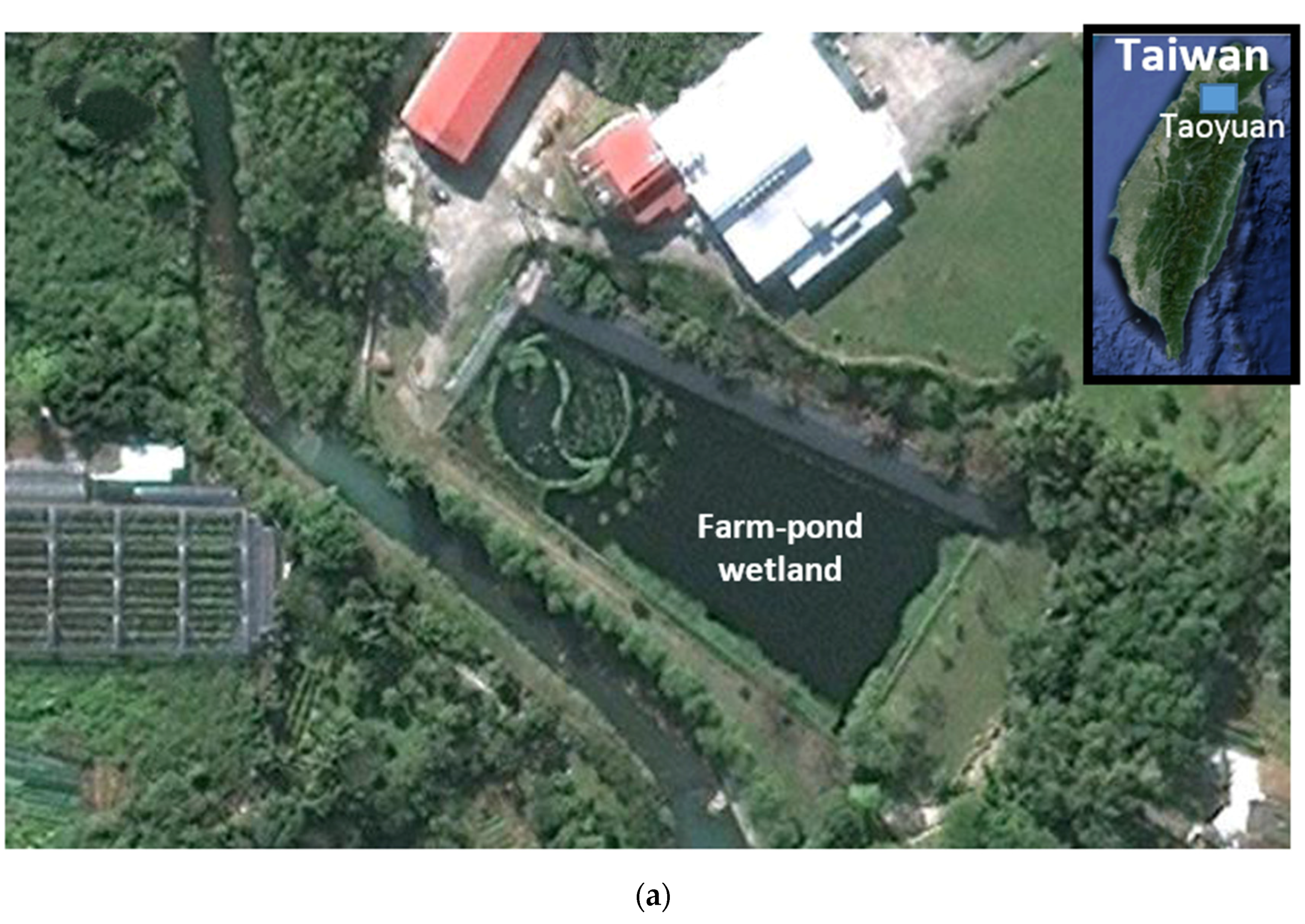
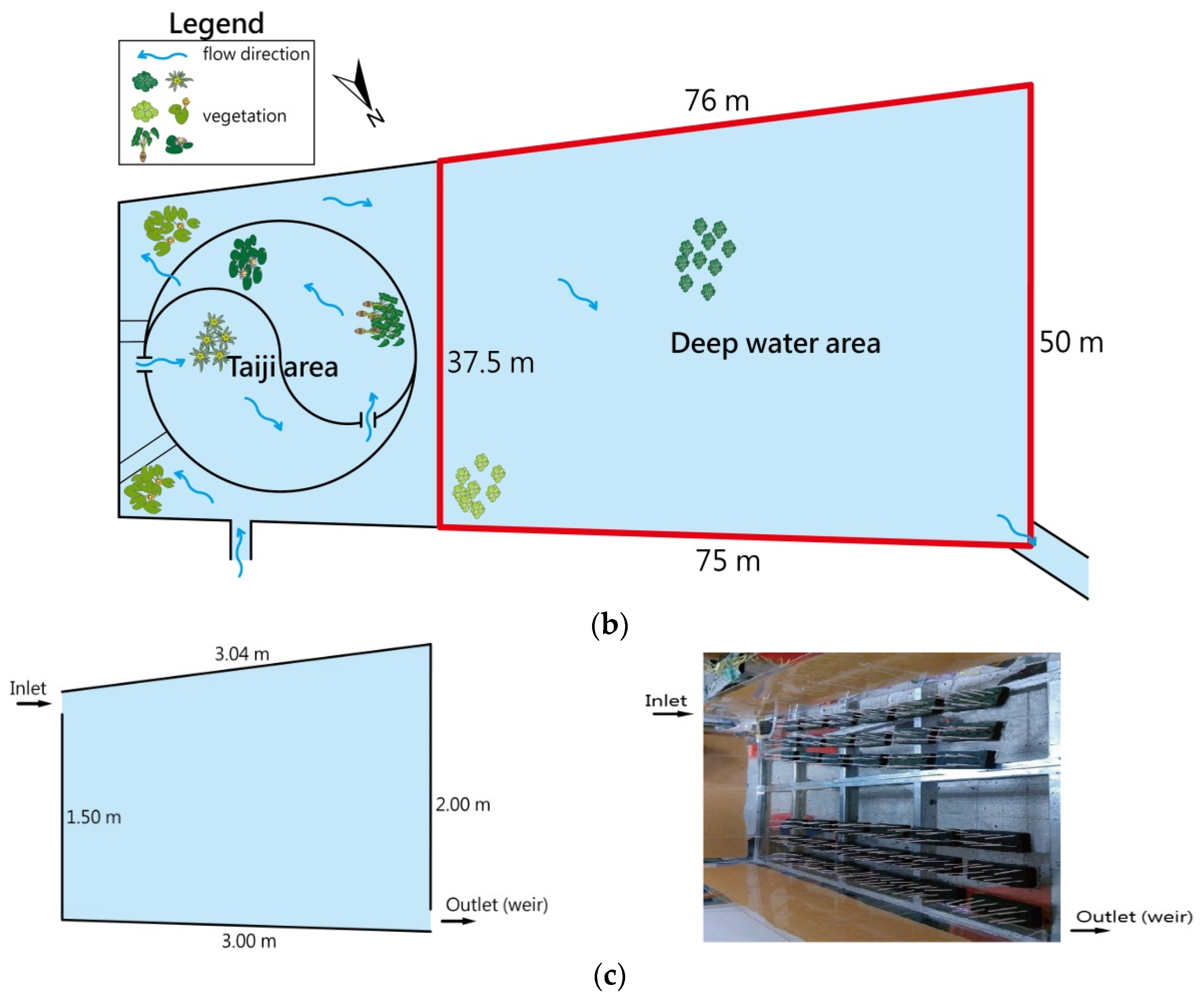
2.1. Study Area
2.2. Flume Experiment Setup
2.2.1. Physical Model
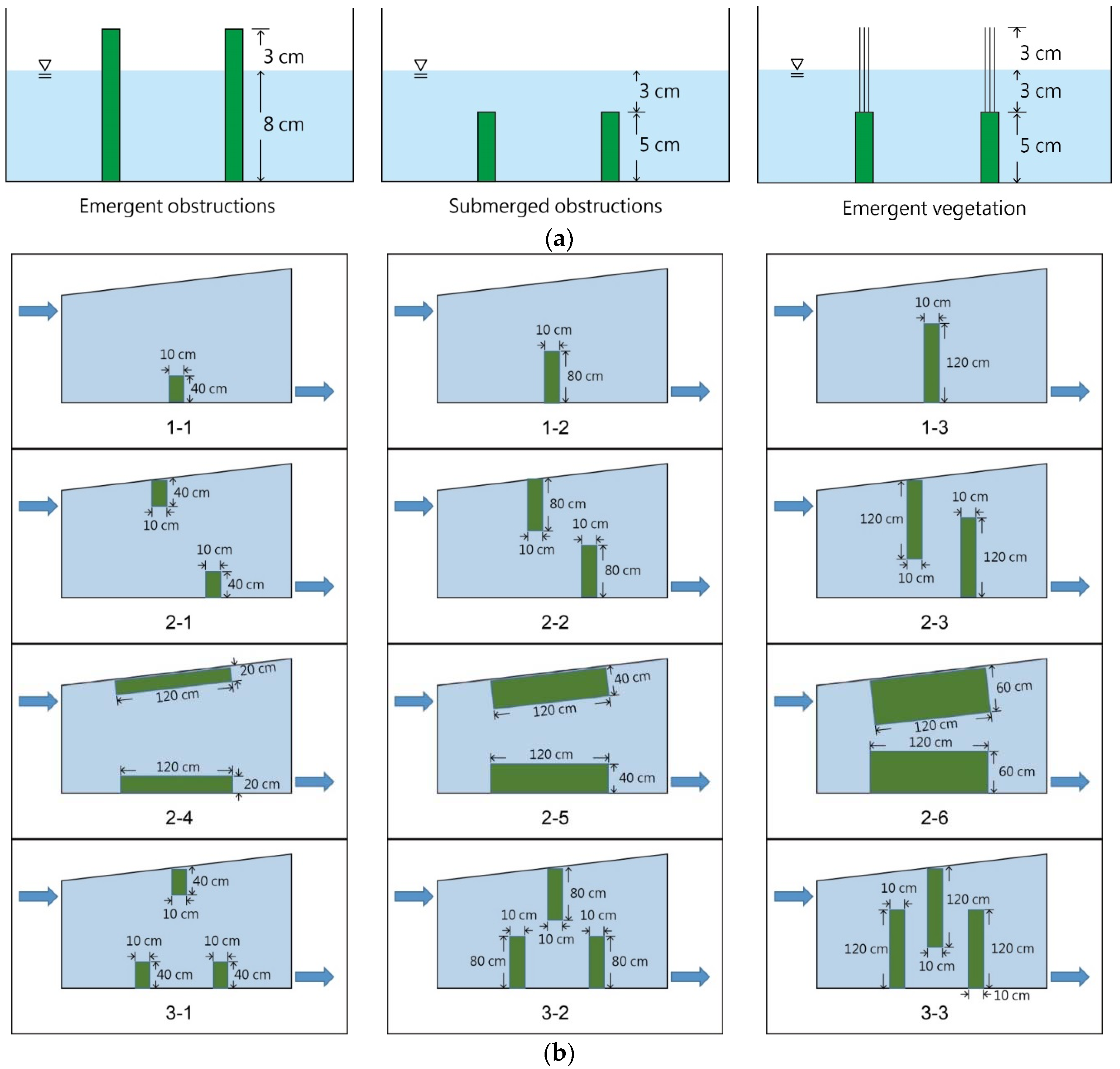
2.2.2. Obstructions and Emergent Vegetation
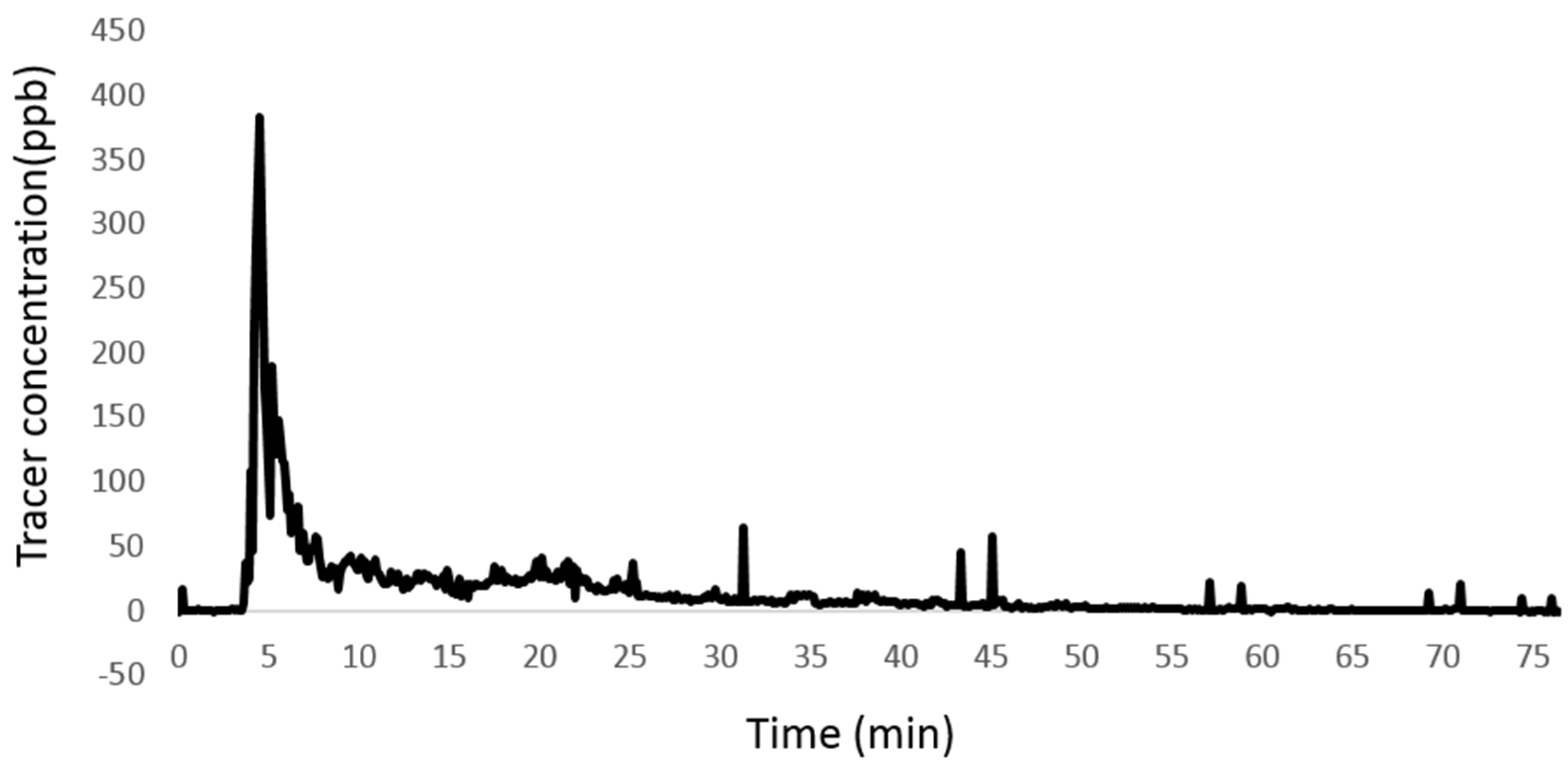
2.2.3. Tracer and Detector
2.3. Residence Time, Effective Volume, and Hydraulic Efficiency
3. Results and Discussion
3.1. No Obstructions or Vegetation
3.2. Installation of Obstructions
3.3. Installation of Emergent Vegetation
3.4. Optimization of Hydraulic Performance
4. Conclusions
Acknowledgments
Author Contributions
Conflicts of Interest
References
- Fogler, H.S. Elements of Chemical Reaction Engineering, 4th ed.; Prentice Hall: Upper Saddle River, NJ, USA, 2006. [Google Scholar]
- Kadlec, R.; Knight, R. Treatment Wetlands; CRC Press, Lewis Publishers: Boca Raton, FL, USA, 1996; p. 892. [Google Scholar]
- Arega, F. Hydrodynamic modeling and characterizing of Lagrangian flows in the West Scott Creek wetlands system, South Carolina. J. Hydro Environ. Res. 2013, 7, 50–60. [Google Scholar] [CrossRef]
- Wang, N.; Mitsch, W.J. A detailed ecosystem model of phosphorus dynamics in created riparian wetlands. Ecol. Model. 2000, 126, 101–130. [Google Scholar] [CrossRef]
- Wahl, M.D.; Brown, L.C.; Soboyejo, A.O.; Dong, B. Quantifying the hydraulic performance of treatment wetlands using the reliability functions. Ecol. Eng. 2012, 47, 120–125. [Google Scholar] [CrossRef]
- Holland, J.F.; Martin, J.F.; Granata, T.; Bouchard, V.; Quigley, M.; Brown, L. Effects of wetland depth and flow rate on residence time distribution characteristics. Ecol. Eng. 2004, 23, 189–203. [Google Scholar] [CrossRef]
- Min, J.; Wise, W.R. Simulating short-circuiting flow in a constructed wetland: The implications of bathymetry and vegetation effects. Hydrol. Process. 2009, 23, 830–841. [Google Scholar] [CrossRef]
- Chang, T.; Chang, Y.; Lee, W.; Shih, S. Flow uniformity and hydraulic efficiency improvement of Deep-Water constructed wetlands. Ecol. Eng. 2016, 92, 28–36. [Google Scholar] [CrossRef]
- Bastviken, S.K.; Weisner, S.E.B.; Thiere, G.; Svensson, J.M.; Ehde, P.M.; Tonderski, K.S. Effects of vegetation and hydraulic load on seasonal nitrate removal in treatment wetlands. Ecol. Eng. 2009, 35, 946–952. [Google Scholar] [CrossRef]
- Keefe, S.H.; Daniels, J.S.T.; Runkel, R.L.; Wass, R.D.; Stiles, E.A.; Barber, L.B. Influence of hummocks and emergent vegetation on hydraulic performance in a surface flow wastewater treatment wetland. Water Resour. Res. 2010, 46, 1–13. [Google Scholar] [CrossRef]
- Persson, J.; Somes, N.L.G.; Wong, T.H.F. Hydraulics efficiency of constructed wetlands and ponds. Water Sci. Technol. 1999, 40, 291–300. [Google Scholar] [CrossRef]
- Shih, S.; Kuo, P.; Fang, W.; LePage, B.A. A correction coefficient for pollutant removal in free water surfacewetlands using first-order modeling. Ecol. Eng. 2013, 61, 200–206. [Google Scholar] [CrossRef]
- Chanson, H. Hydraulics of Open Channel Flow, 2nd ed.; Elsevier Ltd.: Amsterdam, The Netherlands, 2004. [Google Scholar]
- Chang, W.L. The Treatment Efficiency Applying Aquatic Vegetation in Constructed Wetlands; Manual of River Water Quality Improvement Workshop; Environmental Protection Administration: Taipei City, Taiwan, 2006. (In Chinese) [Google Scholar]
- Williams, M.D.; Reimus, P.W.; Vermeul, V.R.; Rose, P.E.; Dean, C.A.; Waston, T.B.; Newell, D.L.; Leecaster, K.B.; Brauser, E.M. Development of Models to Simulate Tracer Tests for Characterization of Enhanced Geothermal Systems; U.S. Department of Energy; Pacific Northwest National: Laboratory: Ridgeland, WA, USA, 2013.
- Su, T.; Yang, S.; Shih, S.; Lee, H.; Su, T.; Yang, S.; Shih, S.; Lee, H. Optimal design for hydraulic efficiency performance of free-water-surface constructed wetlands. Ecol. Eng. 2009, 35, 1200–1207. [Google Scholar] [CrossRef]
- Levenspiel, O. Chemical Reaction Engineering, 3rd ed.; John Wiley & Sons: Hoboken, NJ, USA, 1999. [Google Scholar]
- Thackston, E.L.; Shields, F.D.; Schroeder, P.R. Residence time distributions of shallow basins. J. Environ. Eng. 1987, 113, 1319–1332. [Google Scholar] [CrossRef]
- Dierberg, F.E.; Juston, J.J.; Debusk, T.A.; Pietro, K.; Gu, B. Relationship between hydraulic efficiency and phosphorus removal in a submerged aquatic vegetation-dominated treatment wetland. Ecol. Eng. 2005, 25, 9–23. [Google Scholar] [CrossRef]
- Kadlec, R.H.; Roy, S.B.; Munson, R.K.; Charlton, S.; Brownlie, W. Water quality performance of treatment wetlands in the Imperial Valley, California. Ecol. Eng. 2010, 36, 1093–1107. [Google Scholar] [CrossRef]
- Jenkins, G.A.; Greenway, M. The hydraulic efficiency of fringing versus banded vegetation in constructed wetlands. Ecol. Eng. 2005, 25, 61–72. [Google Scholar] [CrossRef]
- Shih, S.S.; Fang, W.T. Tracer Experiments and Hydraulic Performance Improvements in a Farm Pond Wetland; National Scientific Council: Taipei City, Taiwan, 2013. [Google Scholar]
- USEPA. Manual of Constructed Wetlands Treatment of Municipal Wastewaters; USEPA: Cincinnati, OH, USA, 2000. [Google Scholar]


| Scale Factors | Proportion (Model/Prototype) |
|---|---|
| Length (λL) | 1/25 |
| Time (λT) | 1/625 |
| Velocity (λv) | 25 |
| Discharge (λQ) | 1/25 |
| Data Source | tn | tm | tp | ev | λ | Hydraulic Performance 4 |
|---|---|---|---|---|---|---|
| Flume experiment 1 | 21.87 min | 14.57 min | 4.7 min | 0.66 | 0.22 | Poor |
| Field investigation 2 | 239.58 h | 134.24 h | 76.5 h | 0.56 | 0.32 | Poor |
| Mathematical model simulation 3 | 239.58 h | 135.8 h | 66.5 h | 0.57 | 0.28 | Poor |
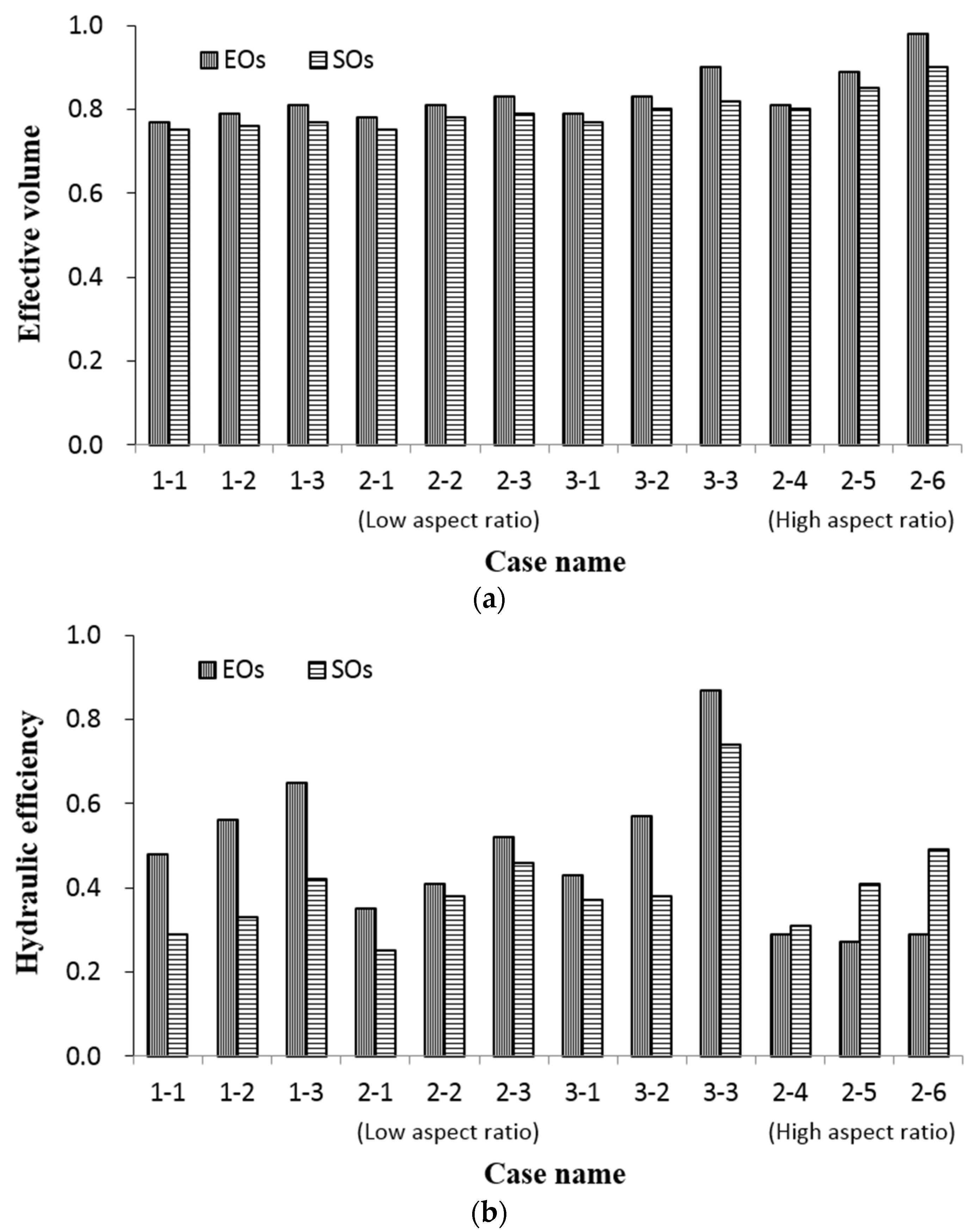
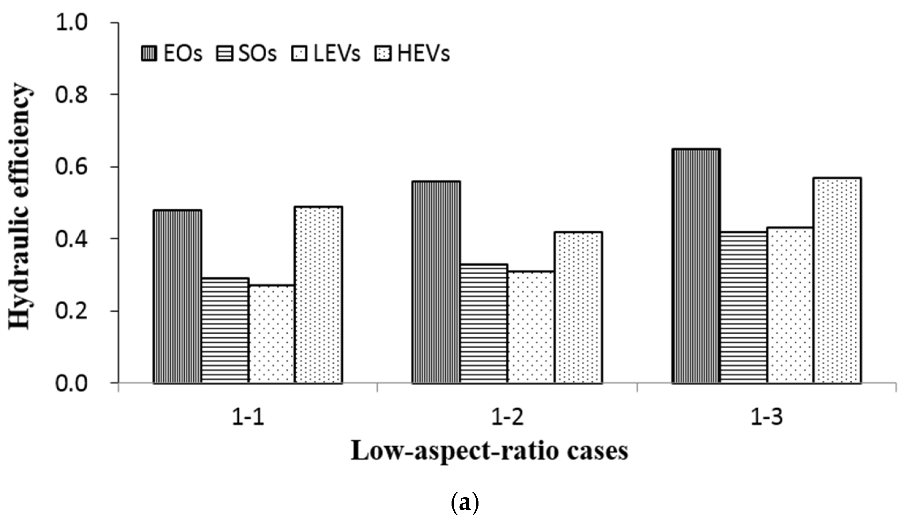
| Cases | tn (min) | tm (min) | tp (min) | ev | λ | Hydraulic Performance | |
|---|---|---|---|---|---|---|---|
| Low aspect ratio | 1–1 | 21.6 | 16.6 | 8.4 | 0.77 | 0.48 | Poor |
| 1–2 | 21.3 | 16.9 | 9.8 | 0.79 | 0.56 | Satisfied | |
| 1–3 | 21.1 | 17.1 | 11.4 | 0.81 | 0.65 | Satisfied | |
| 2–1 | 21.3 | 16.6 | 6.1 | 0.78 | 0.35 | Poor | |
| 2–2 | 20.8 | 16.8 | 7.2 | 0.81 | 0.41 | Poor | |
| 2–3 | 20.3 | 16.9 | 9.1 | 0.83 | 0.52 | Satisfied | |
| 3–1 | 21.1 | 16.7 | 7.6 | 0.79 | 0.43 | Poor | |
| 3–2 | 20.3 | 16.9 | 10.0 | 0.83 | 0.57 | Satisfied | |
| 3–3 | 19.5 | 17.5 | 15.2 | 0.9 | 0.87 | Good | |
| High aspect ratio | 2–4 | 20.3 | 16.4 | 5.0 | 0.81 | 0.29 | Poor |
| 2–5 | 18.7 | 16.6 | 4.8 | 0.89 | 0.27 | Poor | |
| 2–6 | 17.1 | 16.7 | 5.1 | 0.98 | 0.29 | Poor | |
| Cases | tn (min) | tm (min) | tp (min) | ev | λ | Hydraulic Performance | |
|---|---|---|---|---|---|---|---|
| Low aspect ratio | 1-1 | 21.7 | 16.3 | 5.1 | 0.75 | 0.29 | Poor |
| 1-2 | 21.6 | 16.5 | 5.7 | 0.76 | 0.33 | Poor | |
| 1-3 | 21.5 | 16.6 | 7.3 | 0.77 | 0.42 | Poor | |
| 2-1 | 21.6 | 16.2 | 4.4 | 0.75 | 0.25 | Poor | |
| 2-2 | 21.3 | 16.6 | 6.6 | 0.78 | 0.38 | Poor | |
| 2-3 | 21.1 | 16.7 | 8.0 | 0.79 | 0.46 | Poor | |
| 3-1 | 21.5 | 16.5 | 6.4 | 0.77 | 0.37 | Poor | |
| 3-2 | 21.1 | 16.8 | 6.6 | 0.80 | 0.38 | Poor | |
| 3-3 | 20.7 | 17.0 | 12.9 | 0.82 | 0.74 | Satisfactory | |
| High aspect ratio | 2-4 | 21.1 | 16.8 | 5.5 | 0.8 | 0.31 | Poor |
| 2-5 | 20.3 | 17.2 | 7.2 | 0.85 | 0.41 | Poor | |
| 2-6 | 19.5 | 17.5 | 8.1 | 0.90 | 0.49 | Poor | |
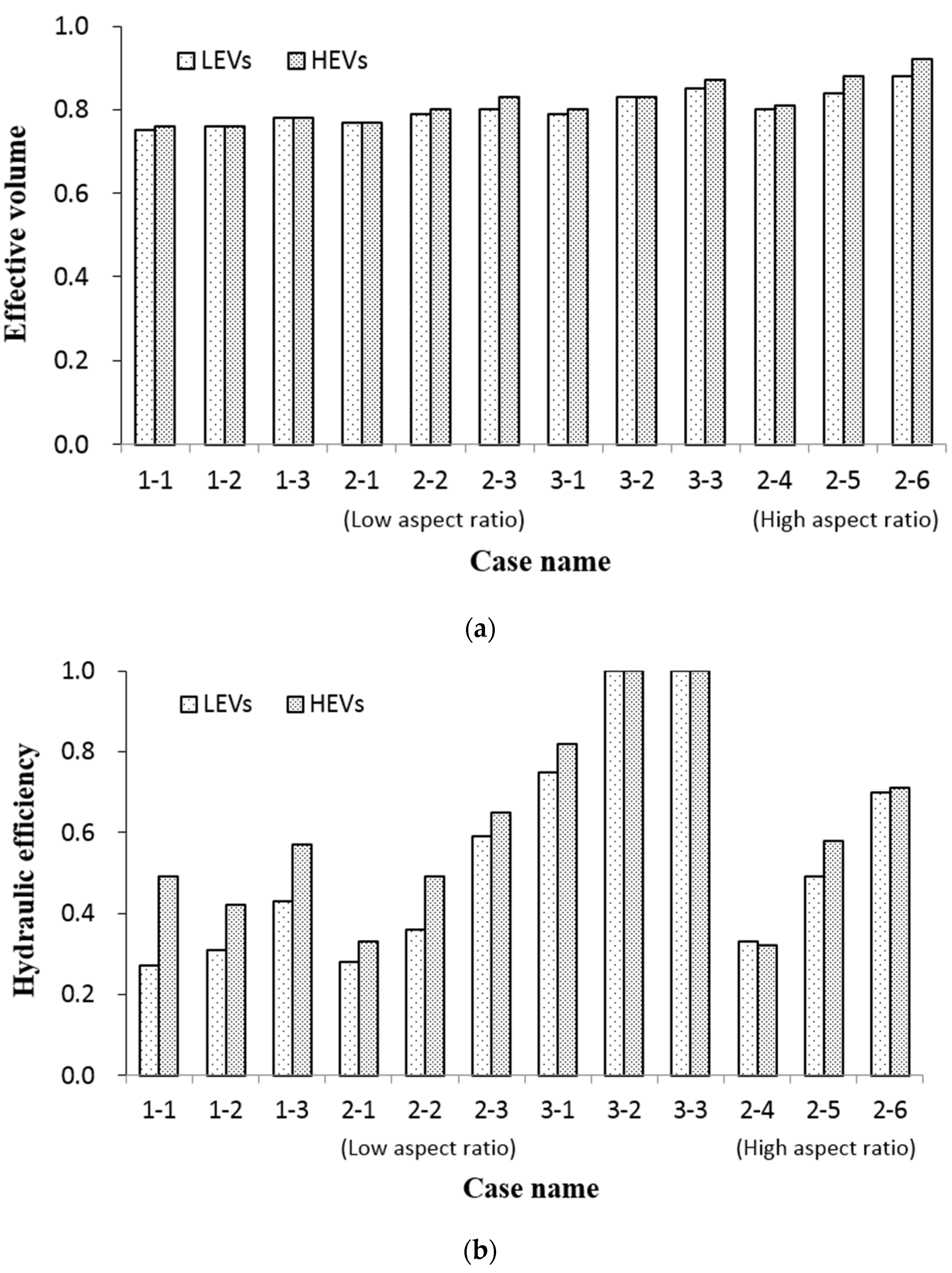
| Cases | tn (min) | tm (min) | tp (min) | ev | λ | Hydraulic Performance | |
|---|---|---|---|---|---|---|---|
| Low aspect ratio | 1-1 | 21.7 | 16.6 | 8.5 | 0.76 | 0.49 | Poor |
| 1-2 | 21.6 | 16.5 | 7.3 | 0.76 | 0.42 | Poor | |
| 1-3 | 21.5 | 16.8 | 9.8 | 0.78 | 0.57 | Satisfactory | |
| 2-1 | 21.6 | 16.7 | 5.7 | 0.77 | 0.33 | Poor | |
| 2-2 | 21.3 | 17.1 | 8.6 | 0.8 | 0.49 | Poor | |
| 2-3 | 21.1 | 17.5 | 11.7 | 0.83 | 0.65 | Satisfactory | |
| 3-1 | 21.5 | 17.1 | 14.3 | 0.8 | 0.82 | Good | |
| 3-2 | 21.1 | 17.6 | 22 | 0.83 | 1 | Good | |
| 3-3 | 20.7 | 17.9 | 21.2 | 0.87 | 1 | Good | |
| High aspect ratio | 2-4 | 21.1 | 17 | 5.6 | 0.81 | 0.32 | Poor |
| 2-5 | 20.3 | 17.8 | 10.2 | 0.88 | 0.58 | Satisfactory | |
| 2-6 | 19.5 | 17.9 | 12.5 | 0.92 | 0.71 | Satisfactory | |
| Cases | tn (min) | tm (min) | tp (min) | ev | λ | Hydraulic Performance | |
|---|---|---|---|---|---|---|---|
| Low aspect ratio | 1-1 | 21.7 | 16.4 | 4.8 | 0.75 | 0.27 | Poor |
| 1-2 | 21.6 | 16.5 | 5.5 | 0.76 | 0.31 | Poor | |
| 1-3 | 21.5 | 16.7 | 7.6 | 0.78 | 0.43 | Poor | |
| 2-1 | 21.6 | 16.6 | 5.0 | 0.77 | 0.28 | Poor | |
| 2-2 | 21.3 | 16.8 | 6.4 | 0.79 | 0.36 | Poor | |
| 2-3 | 21.1 | 16.9 | 10.3 | 0.80 | 0.59 | Satisfactory | |
| 3-1 | 21.5 | 17.0 | 13.2 | 0.79 | 0.75 | Good | |
| 3-2 | 21.1 | 17.4 | 21.4 | 0.83 | 1.00 | Good | |
| 3-3 | 20.7 | 17.6 | 18.1 | 0.85 | 1.00 | Good | |
| High aspect ratio | 2-4 | 21.1 | 16.8 | 5.8 | 0.80 | 0.33 | Poor |
| 2-5 | 20.3 | 17.1 | 8.6 | 0.84 | 0.49 | Poor | |
| 2-6 | 19.5 | 17.2 | 12.2 | 0.88 | 0.70 | Satisfactory | |
© 2016 by the authors; licensee MDPI, Basel, Switzerland. This article is an open access article distributed under the terms and conditions of the Creative Commons Attribution (CC-BY) license (http://creativecommons.org/licenses/by/4.0/).
Share and Cite
Shih, S.-S.; Hong, S.-S.; Chang, T.-J. Flume Experiments for Optimizing the Hydraulic Performance of a Deep-Water Wetland Utilizing Emergent Vegetation and Obstructions. Water 2016, 8, 265. https://doi.org/10.3390/w8060265
Shih S-S, Hong S-S, Chang T-J. Flume Experiments for Optimizing the Hydraulic Performance of a Deep-Water Wetland Utilizing Emergent Vegetation and Obstructions. Water. 2016; 8(6):265. https://doi.org/10.3390/w8060265
Chicago/Turabian StyleShih, Shang-Shu, Shang-Shang Hong, and Tsang-Jung Chang. 2016. "Flume Experiments for Optimizing the Hydraulic Performance of a Deep-Water Wetland Utilizing Emergent Vegetation and Obstructions" Water 8, no. 6: 265. https://doi.org/10.3390/w8060265