Article

The Influence of the Annual Number of Storms on the Derivation of the Flood Frequency Curve through Event-Based Simulation

1
Civil Engineering Department, Hydraulics, Energy and Environment, Technical University of Madrid, Madrid 28040, Spain
2
AQUATEC, Proyectos para el Sector del Agua, S.A.U. (Suez Group), Madrid 28037, Spain
*
Author to whom correspondence should be addressed.
Water 2016, 8(8), 335; https://doi.org/10.3390/w8080335
Submission received: 27 May 2016 / Revised: 26 July 2016 / Accepted: 29 July 2016 / Published: 5 August 2016

Abstract

:
This study addresses the question of how to select the minimum set of storms that should be simulated each year in order to estimate an accurate flood frequency curve for return periods ranging between 1 and 1000 years. The Manzanares basin (Spain) was used as a study case. A continuous 100,000-year hourly rainfall series was generated using the stochastic spatial–temporal model RanSimV3. Individual storms were extracted from the series by applying the exponential method. For each year, the extracted storms were transformed into hydrographs by applying an hourly time-step semi-distributed event-based rainfall–runoff model, and the maximum peak flow per year was determined to generate the reference flood frequency curve. Then, different flood frequency curves were obtained considering the N storms with maximum rainfall depth per year, with 1 ≤ N ≤ total number of storms. Main results show that: (a) the degree of alignment between the calculated flood frequency curves and the reference flood frequency curve depends on the return period considered, increasing the accuracy for higher return periods; (b) for the analyzed case studies, the flood frequency curve for medium and high return period (50 ≤ return period ≤ 1000 years) can be estimated with a difference lower than 3% (compared to the reference flood frequency curve) by considering the three storms with the maximum total rainfall depth each year; (c) when considering only the greatest storm of the year, for return periods higher than 10 years, the difference for the estimation of the flood frequency curve is lower than 10%; and (d) when considering the three greatest storms each year, for return periods higher than 100 years, the probability of achieving simultaneously a hydrograph with the annual maximum peak flow and the maximum volume is 94%.

Graphical Abstract

1. Introduction

For the design of hydraulic infrastructures, peak-flow frequency curves (FFCs) ranging return periods higher than the duration of the observed data are often needed. The use of statistical procedures is common (e.g., [1,2,3,4,5]). Moreover, given the lack of data (or as a complementary analysis), event-based rainfall–runoff models starting from rainfall data, generally with longer observed spatial–time series than the hydrometric ones (e.g., [6,7,8,9,10,11,12]), are applied. Those models are used in order to obtain the flood hydrographs from rainfall information. A possible methodological approach applied by several authors consists in the estimation of the peak-flow frequency curves based on stochastic rainfall models coupled with deterministic rainfall–runoff models following either a continuous-time or event-based approach [13,14,15,16,17,18,19]. Even though the continuous rainfall–runoff models estimate the variables for the entire period of simulation, they usually require intensive input data, are more complex to implement and calibrate, and have some limitations due to the intensive computational demands, particularly when peak-flow annual maxima are needed for high return periods (Tr). Contrarily, event-based rainfall–runoff models generally require less input data, are easily applicable and, according to some authors, are affected by fewer errors and total uncertainties (e.g., [20]). However, the use of event-based models for the FFC estimation has some drawbacks. Some authors have suggested the storm volume and duration (including the identification of the storm events), its spatial distribution and the antecedent soil moisture [21,22,23] as determinant factors for the estimation of the flow quantile. This paper deals with the first three factors. The antecedent soil moisture condition, in professional practice, is usually assumed as deterministic. Many authors have achieved good results considering the antecedent soil moisture condition as a random variable associated to a probability distribution function [16,24,25,26]. Recently, Flores-Montoya et al. [24] proposed a probabilistic approach that considered the initial state as a random variable characterized by a probability distribution determined through Monte Carlo simulation. The results of this approach were compared to the results using a fixed average initial condition. Although the probabilistic approach produced slightly better results, the results of the deterministic approach were also good. In addition, it is common to assume that the same probability of occurrence adopted for the precipitation is also associated to the peak flow, a hypothesis that is not necessarily true [27,28,29]. Then, an additional critical aspect using event-based models is the determination of the rainfall event that generates the annual maximum peak flow. In fact, for the estimation of peak-flow frequency curves using probabilistic approaches, various authors have suggested a minimum sample size with ratios between the maximum Tr of the sample and the maximum Tr to be estimated no less than 10 or 20 (e.g., [18,30]). Thus, if a representative sample for the estimation of the upper range of the peak-flow frequency curve for high Tr is needed (Tr between 100 and 1000 years), the performance of several simulations to ensure the inclusion of the storm that generates the maximum flow each year would be required, resulting computationally expensive [31]. This study focuses on the selection of the minimum set of storms that should be extracted and simulated each year (in event-based models) in order to ensure obtaining the peak flow each year.
With respect to the characterization of precipitation, in professional practice, a single design storm is defined as a storm that produces the design flood. The procedure for the storm-generation usually introduces a single probabilistic concept corresponding to the probability of the occurrence of a certain amount of accumulated precipitation for a specific storm duration. Although most of the physical processes are defined deterministically according to the criteria of the designer, many of the involved variables have a stochastic nature, for example the duration of the storms, the accumulated volume, the temporal and spatial distribution and recurrence of rainfall events, among others. Additionally, the assumption is made that the likelihood of occurrence of the design flood is the same one adopted for the design storm, a hypothesis that is not necessarily true [27,28,29]. The application of stochastically generated rainfall models can consider the stochastic nature of many of the mentioned variables. The Neyman–Scott and Bartlett–Lewis models based on rectangular pulses, which have been applied to the temporal simulation of precipitation at a single site, are the most widely used [32,33,34]. Other approaches show promising results, for example those based on the theory of copulas that correlate variables such as the storm duration, average intensity or rainfall volumes (e.g., [35,36,37,38]. These models are capable of performing hourly disaggregation based on daily data with an acceptable degree of adjustment. Moreover, in many cases, spatial rainfall correlation is expected. There are stochastic rainfall models that can disaggregate the rainfall process while keeping the spatial correlation structure. Continuous stochastic space–time models for generation of simulated precipitation are currently being developed with promising results (e.g., [39,40,41,42]).
Regarding rain event identification, a diversity of approaches can be found [43,44,45,46]. Rain events are commonly delimited by setting the required duration of a rainless interval that precedes and follows a rain event (MIT, minimum inter-event time). However, in many studies, the criterion for the identification of independent rainfall events is not clearly stated [43]. Besides arbitrary criteria for identifying storms within a continuous rainfall series, there are some methods based on rainfall processes, such as rank correlation, autocorrelation and exponential method [44]. They concluded that the exponential method, proposed by Restrepo-Posada and Eagleson [45], may be appropriate to determine the value of MIT for studies where catchment antecedent conditions are relevant. The exponential method is based on the assumption that the arrivals of independent rainstorms correspond to a Poisson process. Therefore, it can be expected that storm arrival time and the time between storms follows an exponential distribution. The method proposes to gradually increase the MIT until finding the value that provides a coefficient of variation (CV) equal to one. Once this condition is achieved, resulting storms can be assumed as independent [45,46].
Summarizing, a possible methodological approach to estimate the peak-flow frequency curves from rainfall information is based on the application of stochastic rainfall models coupled with deterministic rainfall–runoff models. The ideal scenario would be the use of a continuous-time spatial–temporal stochastic rainfall generator followed by a distributed continuous-time rainfall–runoff model. However, this methodology has some limitations (above mentioned) that hinder its application, particularly for the analysis of high return periods that require long simulation periods. Other alternative is the use of a continuous-time spatial–temporal stochastic rainfall generator followed by a distributed or semi-distributed event-based rainfall–runoff model. Given that the return period of the generated storms is not necessarily the same as that of the derived hydrographs, the simulation of several storms per year would be required to determine the annual maximum peak-flow. The aim of this study is to address the question of storm selection for the generation of the FFC through event-based rainfall–runoff models: how to select the minimum set of storms that should be extracted and simulated each year in order to ensure obtaining the peak flow each year and generate an accurate annual FFC for Tr ranging between 1 and 1000 years.

2. Materials and Methods

Figure 1 shows the general conceptual framework of the proposed methodology. The methodology can be summarized by the characterization of the main processes as follows: (a) continuous stochastic rainfall generation; (b) identification of independent storms for each simulated year; (c) hydrographs and peak flows calculation; and (d) determination and comparison of several flood frequency curves by considering different number of storms each year.

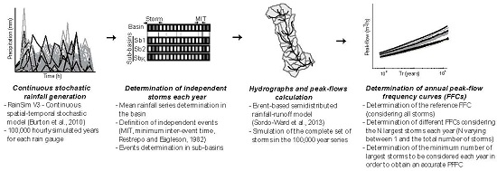
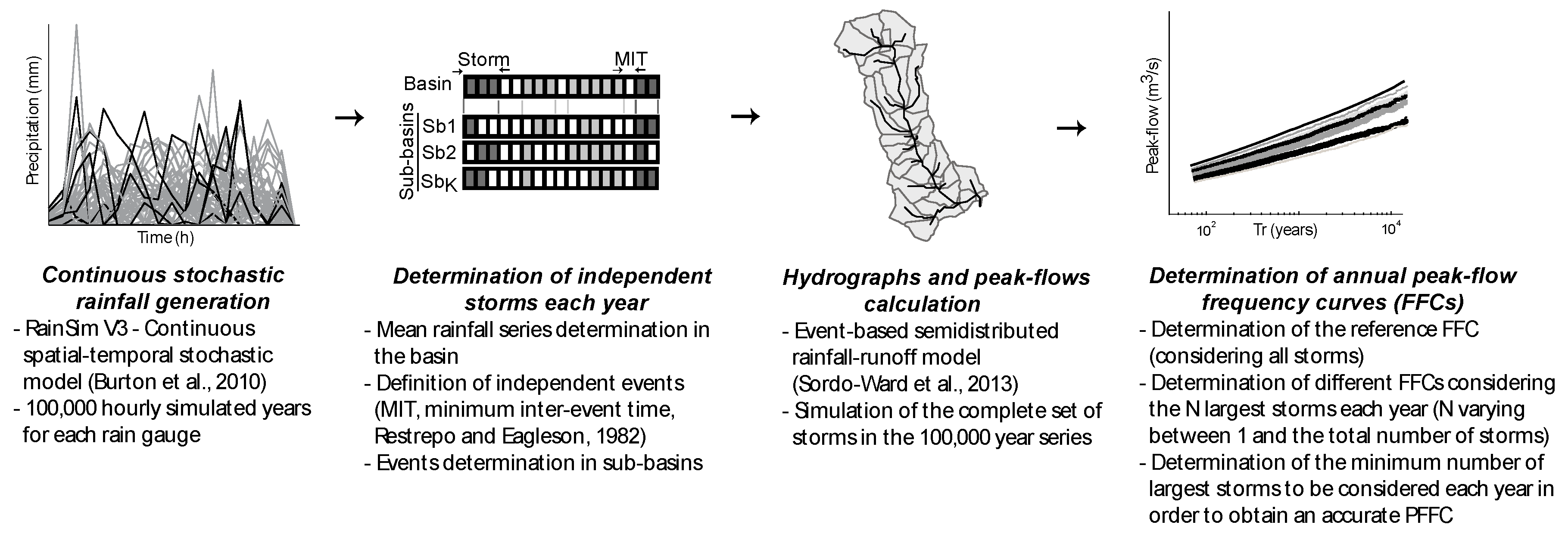
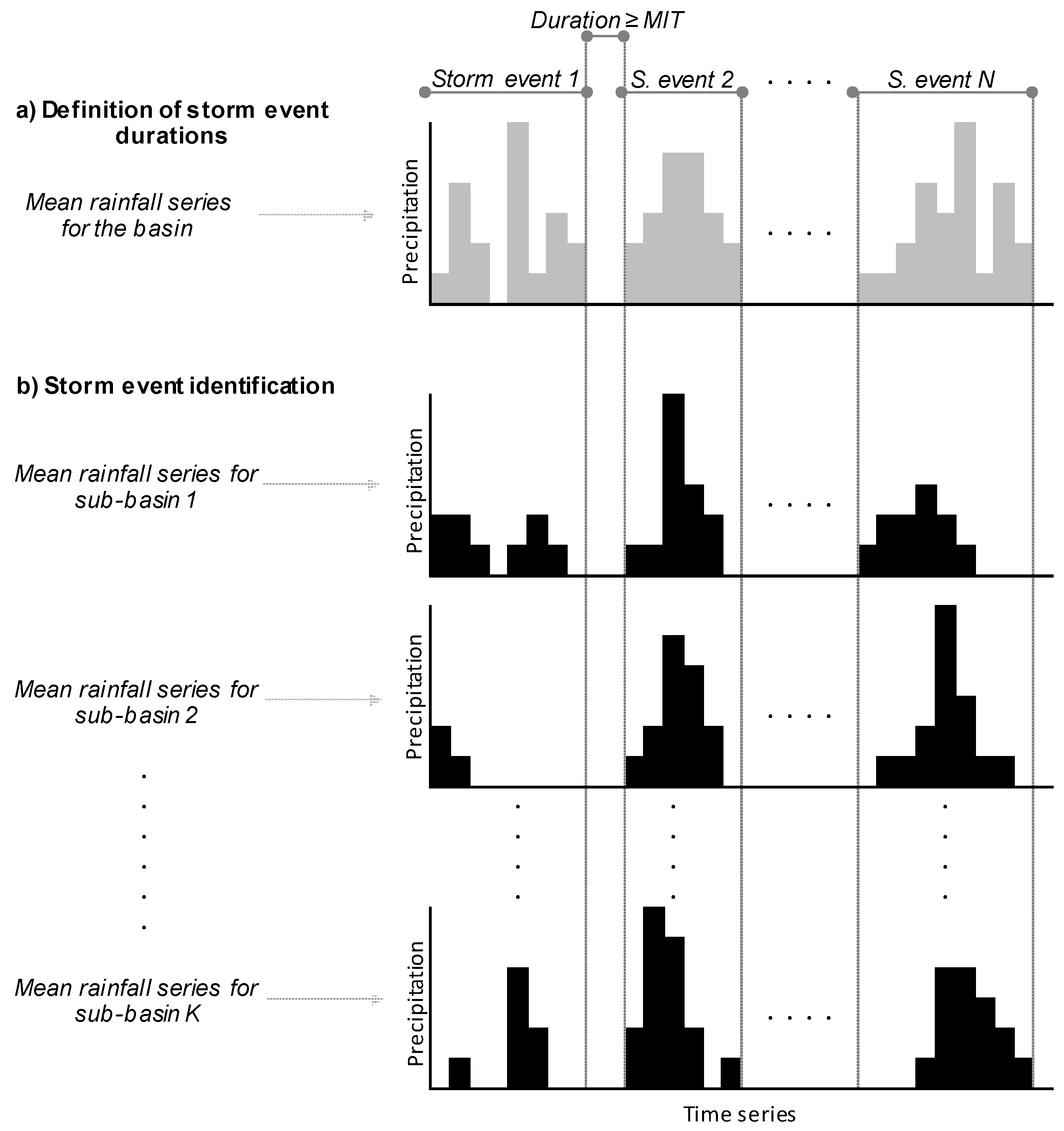
2.1. Stochastic Rainfall Series Generation and Storm Identification

We performed a continuous stochastic spatial–temporal modeling by applying the RainSimV3 [39,40]. We generated hourly continuous rainfall series arbitrarily long for each rain gauge location. RainSimV3 is based in the model of generation of rectangular pulses of Neyman–Scott [42]. Such models are able to capture the main observed rainfall time-series statistic characteristics; for the case of the RainSimV3 model: (1) mean waiting time between adjacent storm origins (h); (2) mean waiting time for rain cell origins after storm origin (h); (3) mean duration of rain cell (h); (4) mean intensity of a single rain cell (mm/h); (5) mean radius of rain cells (km); (6) spatial density of rain cell centers (km−2); and (7) a vector of scale factors, one for each rain gauge (-). Generally, the available observed data in the basin consist of daily rainfall series. From these data, the model is calibrated by applying the Shuffled Complex Evolution algorithm [47], in order to adjust the model rainfall time-series statistic characteristics to the behavior of the observed daily rainfall series. A detailed description of the RainSimV3 can be found in Burton et al. [39]. The stochastic rainfall model validation was performed comparing both the annual maximum daily rainfall frequency curve from observed data in each rain gauge and simulated from the model at the same location. We obtained the daily modeled values by aggregating the hourly simulated time-series.
By applying the Thiessen polygon method, we determined the mean hourly time-series for the entire basin and period of analysis. From this time-series we identified and extracted the storms. The minimum inter-event time (MIT) of no rain between two storm events to be considered as independent events was determined by applying the exponential method [46]. By applying the criteria of the total rainfall depth, we sorted them each year from the highest (and named storm of order 1 of the year) to the lowest [48] (Figure 2a). Then, for the identified event periods we determined the mean storm event for each defined sub-basin by applying the Thiessen polygon method (Figure 2b). Therefore, there is simultaneity among storms of different sub-basins; however, these storms might be different depending on their total depth and temporal distribution. By applying the rainfall–runoff model [49,50], we obtained the hydrographs at the basin outlet. Finally, we calculated different FFCs varying the number of the largest storms considered each year between one and the whole number of occurred storms, ensuring the inclusion of the storm which generates the flood with the annual maximum peak flow.

2.2. Estimation of the Peak Flow Frequency Curves
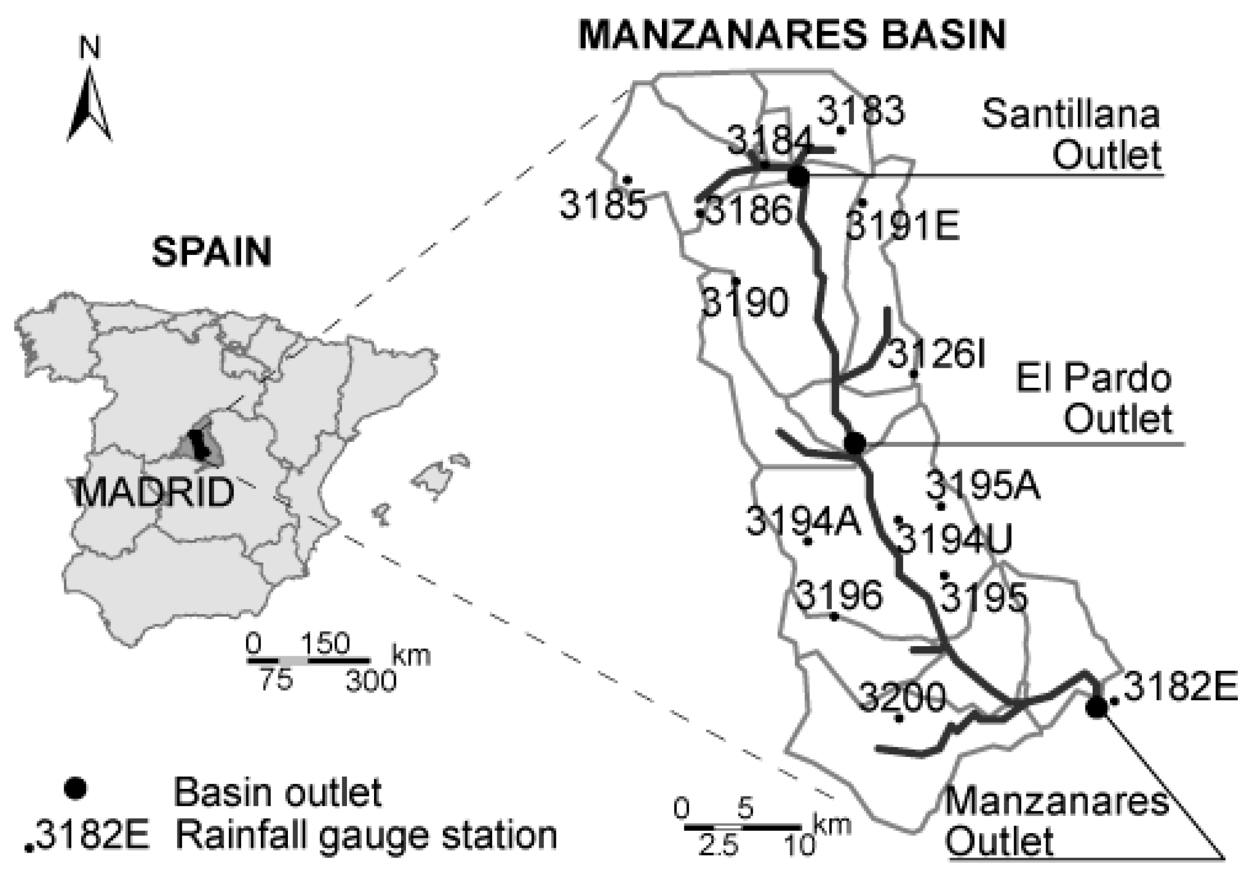
Once all hyetographs for each sub-basin were obtained, we calculated the hydrographs at the basin outlet by applying an hourly time-step semi-distributed event-based hydrological model [49,50,51]. A chain of models designed to simulate the main physical processes was used. The curve number method was applied for the rainfall–runoff transformation [52] and the hydrographs were generated by using the Soil Conservation Service dimensionless unit hydrograph procedure [52]. We adopted the simpler option of deterministic average initial conditions based on the results of Flores-Montoya et al. [24]. For the propagation of the flood hydrographs throughout the stream channels, the Muskingum method was applied [53]. The values of the parameters used in this study were extracted from Sordo-Ward et al. [27]. A detailed description of the hydrologic model may be found in Sordo-Ward et al. [27].
For each year, we sorted the identified storms from highest to lowest according to three criteria: (a) the total rainfall depth; (b) the storm duration; and (c) the mean storm intensity. The largest storm each year was identified as order 1; the second largest storm as order 2, and so on until covering the total number of selected storms each year. This was named as the reference flood frequency curve (FFCR). We performed the rainfall–runoff simulations for storms selected under all three criteria. For each criterion, we identified the order of storm event that generated the maximum peak flow in that year, and compared the storm orders obtained for each criterion and for the entire period analyzed. We selected as the best criterion the one that required lower storm orders for obtaining the peak-flow annual maxima (as will be shown later, in this study, the selected criterion was the total rainfall depth). Then, based on the selected criterion, we calculated different FFCs varying the number of storm events considered each year. First, we selected the largest storm each year (storm of order 1); second, we considered the two largest storms of each year (order 1 + order 2) and so on until covering the total number of selected storms per year. Finally, we compared the FFCs and determined the minimum number of storms to be considered each year in order to ensure the inclusion of the annual maximum peak flow.

2.3. Case Studies

The methodology was applied to three basins located in the Manzanares River basin (with a total area of 1294 km2), a tributary of the Targus River in the central region of mainland Spain. The studied basins were: Santillana (211 km2), El Pardo (495 km2) and Manzanares (1294 km2). The sub-basin determination was conducted according to Sordo-Ward et al. [27]. The main characteristics are summarized in Table 1 and Figure 3.
We used daily data from 14 rain gauges (Figure 3) with time series lengths varying between 26 and 112 years. By applying the methodology, for each rain gauge location, we generated 100,000-year time series of rainfall with hourly time-step. By applying the Thiessen polygon method, a 100,000-year continuous mean rainfall series (hourly step) was obtained for the entire basin. The minimum inter-event time (MIT) to consider independent storms was 33 h. It was calculated by applying the exponential method proposed by Restrepo-Posada and Eagleson [46]. Then, we defined the starting time and duration of around 2,500,000 storms and identified, for each sub-basin, the correspondent hyetographs. This implies a ratio of 100 between the maximum Tr of the sample and the maximum Tr to be estimated, which ensured obtaining a representative sample to estimate the FFCs for the entire range considered [18,30]. Each year, we sorted them from highest to lowest according to the three mentioned criteria and selected the total rainfall depth as the most relevant one (as will be shown later). Finally, the individual events were all simulated. Given that the return period of the storms is not necessarily the same as that of the derived hydrographs, we estimated 25 FFCs (with a Tr ranging between 1 and 1000 years). First, we considered the storms of order 1 each year (estimating the FFC1), second the storms of order 1 + 2 (FFC2), and so on until considering 25 storms each year. This was considered the reference flood frequency curve (FFCR). In all cases, for each year, the annual maximum peak-flow was identified and the corresponding FFC was estimated by applying the Gringorten non-parametric formula. The basin characteristics, sub-basin determination, topology, deterministic average initial conditions and parameters were selected from Sordo-Ward et al. [27]. In addition, for comparison purposes, we used hourly data from six storm events in the Manzanares basin recorded by five rain gauges and the corresponding observed hydrographs at the Manzanares basin outlet (gauge station 3182E). We simulated the storm events and compared the peak flows with the observed ones.

2.4. Limitations of the Methodology

The methodology and models applied have certain limitations that should be noted. First, the analysis has been done only in three basins, which may limit generalizations of the results and conclusions. Second, the study is focused in Tr ranging between 1 and 1000 years. If other range of Tr is analyzed, the size of the generated rainfall series should be analyzed to ensure obtaining a representative sample to estimate the FFCs [18,30]. However, the uncertainty of the process is linked to the ratio between the length of the observed series used to calibrate the stochastic rainfall model and the length of the synthetic series generated. It should be noted that the rainfall series were generated taking into account the statistic characteristics of the observed daily rainfall series (observed series are no longer than 100 years), and therefore 1000 years seems a reasonable upper limit for extrapolation. Moreover, the procedure did not consider climate change effects or possible long-term variations of rainfall. Finally, we adopted the simpler option of deterministic average of the initial soil moisture conditions based on the results of Flores-Montoya et al. [24].

3. Results and Discussion

In this section, we present the rainfall model calibration/validation and the rainfall events identification/characterization. Subsequently, we estimate the FFCs by applying a semi-distributed event-based hydrological model. Then, we analyze the effect of considering different number of storms each year on the degree of alignment between the calculated flood frequency curves and the reference flood frequency curve. Additionally, we perform a joint analysis of the maximum annual peak flow and hydrograph volume. Finally, we analyze the effect of considering different inter-storm times on the FFCs estimation.

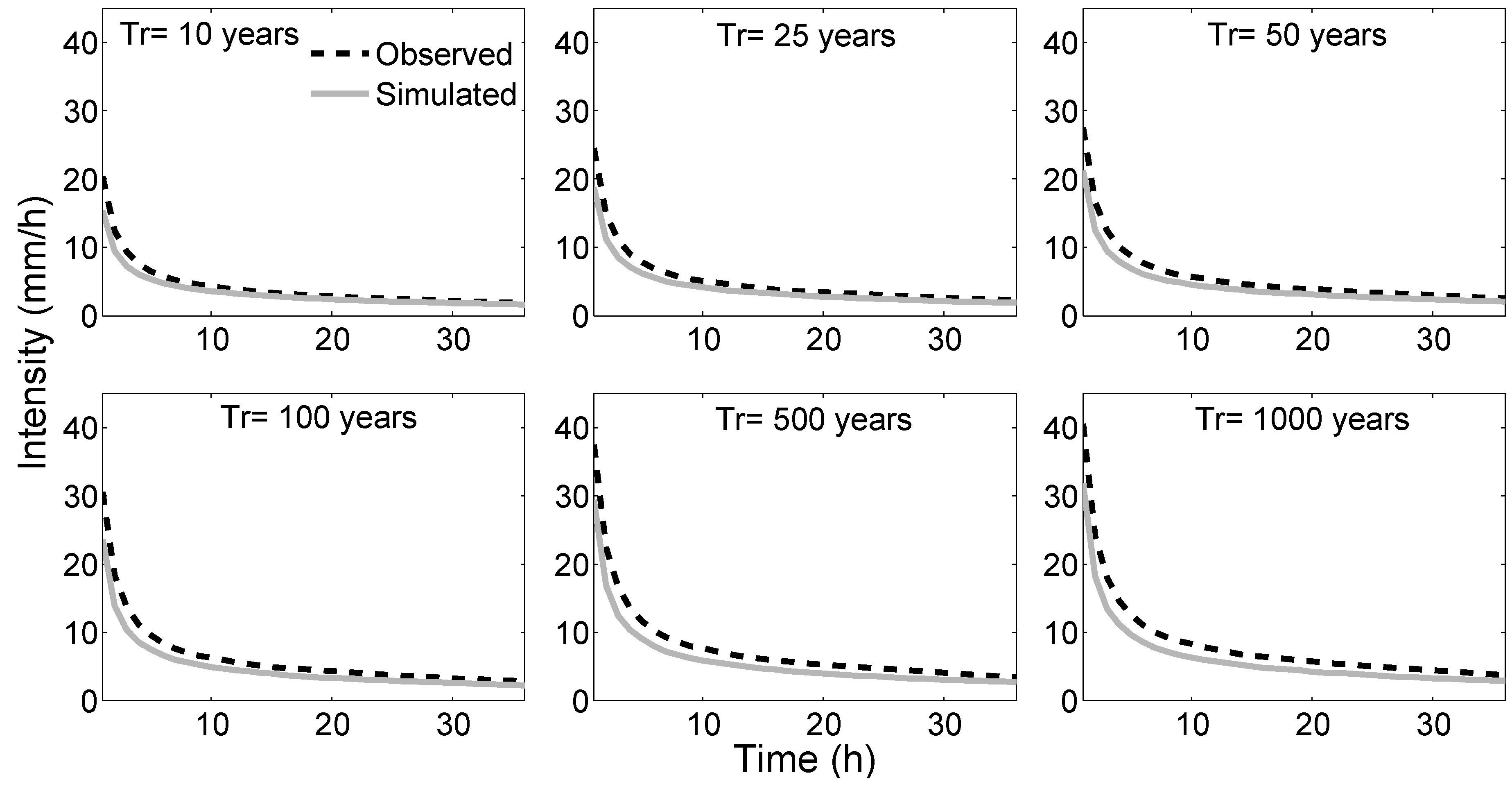
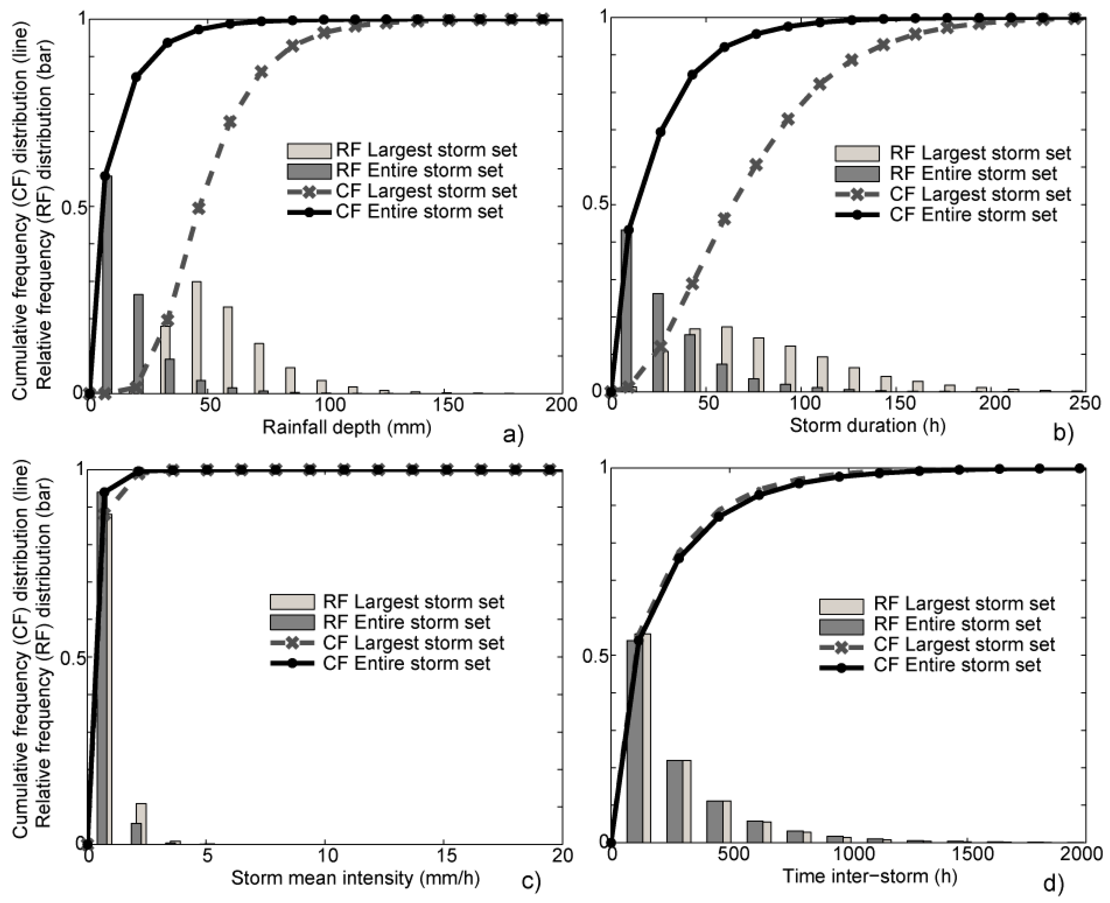
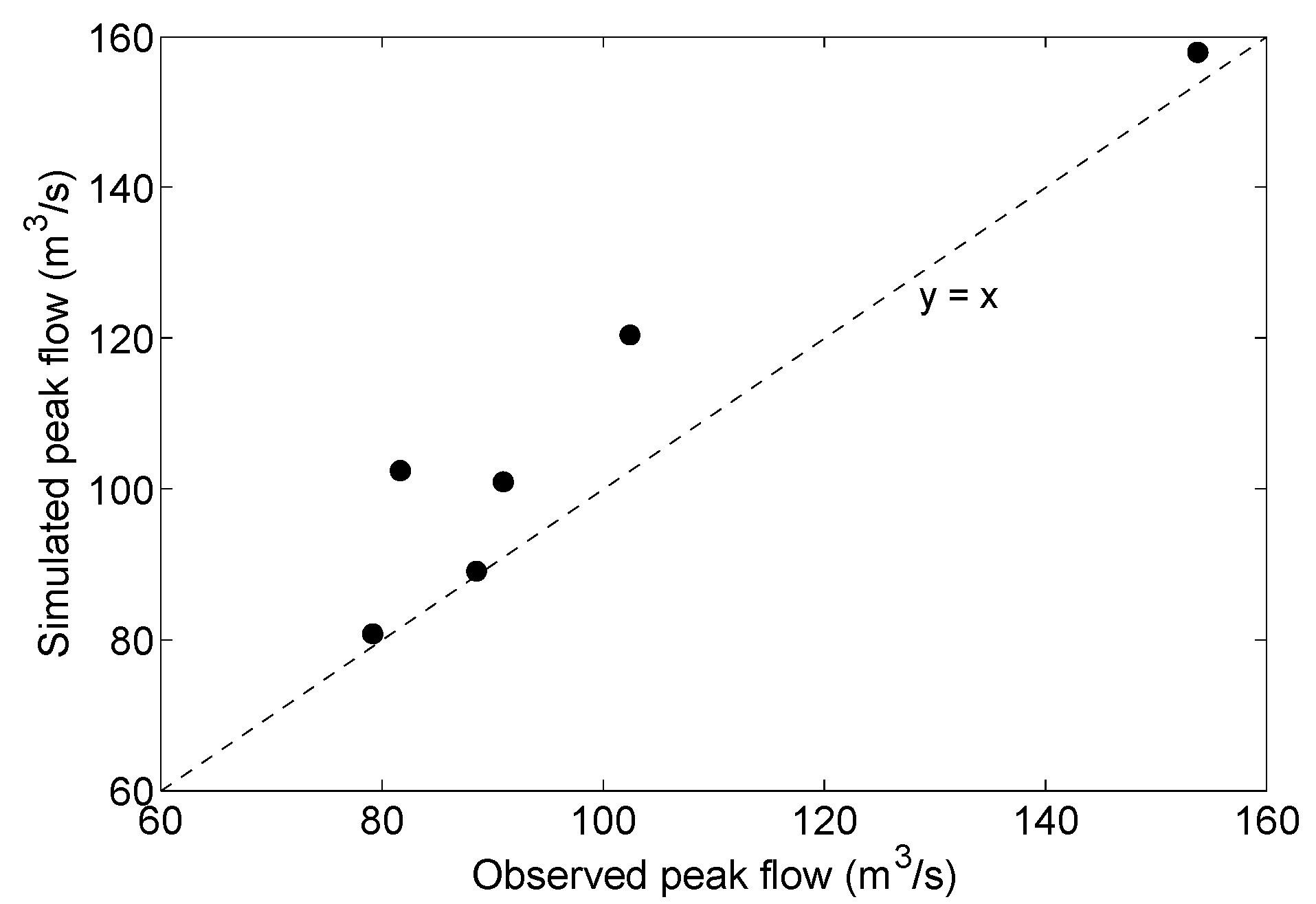
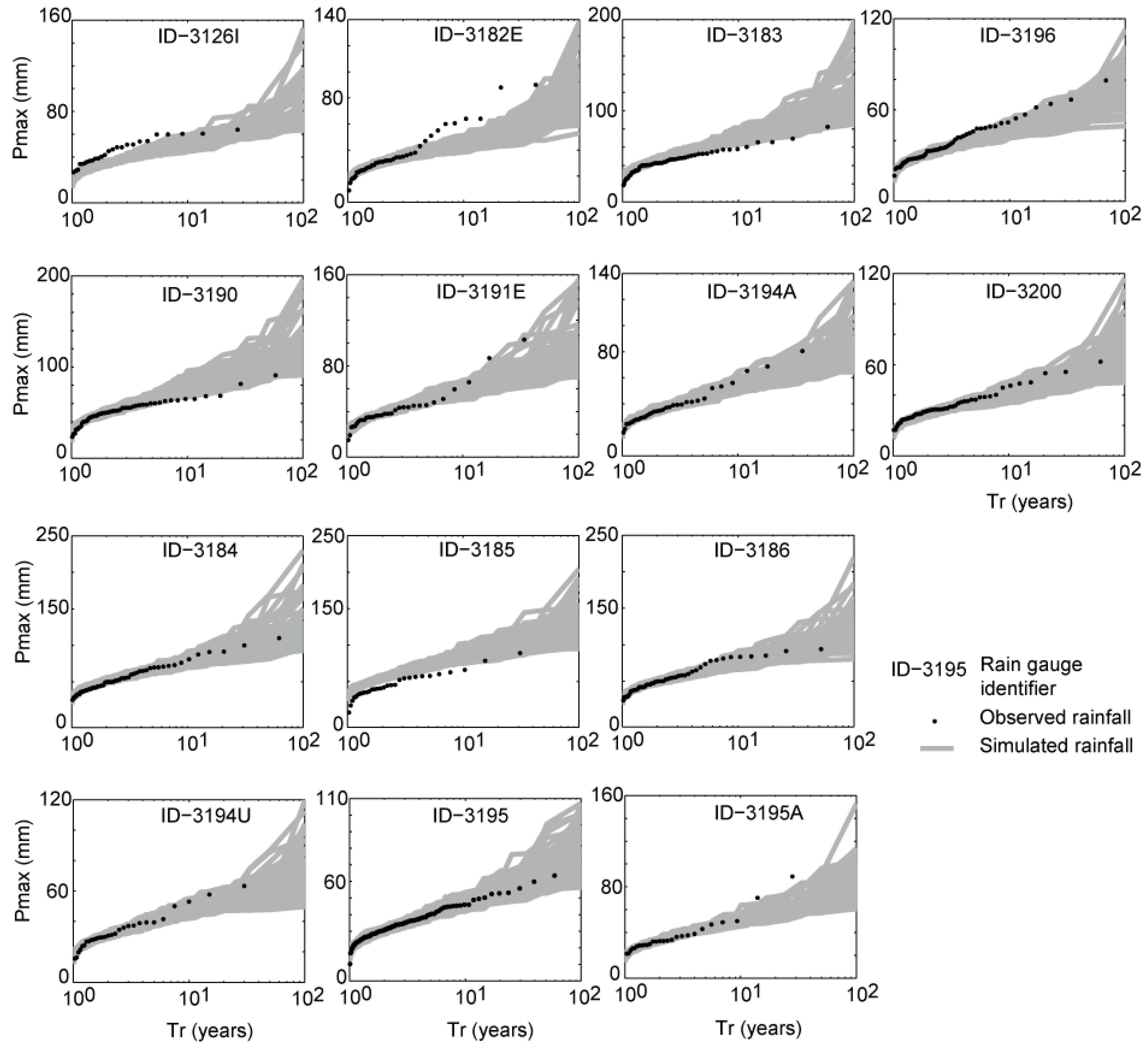
3.1. Rainfall Model Calibration/Validation and Rainfall Events Identification/Characterisation

As stated, the calibration was conducted by applying the Shuffled Complex Evolution algorithm [47] in order to adjust the model rainfall time-series characteristic statistics to the behavior of the observed daily rainfall series for the 14 rain gauge locations [39]. It should be noted that the calibration and rainfall simulation were realized considering temporal and spatial correlation among gauges. Figure 4 shows the validation of the stochastic rainfall model. It was performed by comparing the annual maxima for the daily rainfall frequency curves obtained from observed and simulated values (we generated 60 hourly series of 100 years). As shown, the behavior of the observed rainfall frequency curves was mostly within the range of the simulated ones. Results largely fulfilled our aim of generating arbitrary long rainfall series (100,000 years) with extreme behaviors of the same order than the observed ones.
Although, in most rainfall stations, the available data have daily time-step, for rainfall station ID-3195, a 60-year time-series with a 5-min time-step was available. For this location, we calculated the Intensity–Duration–Frequency curves (IDF) for the observed and simulated data (return periods: 10, 25, 50, 100, 500 and 1000 years). Figure 5 shows the comparison of the IDF in both cases. We considered storm durations ranging between 5 min and 36 h for the observed time-series and between 1 and 36 h for the simulated data. Each year, the storms were extracted from the entire continuous rainfall series. For each considered storm duration and each year, the largest rainfall depth storm was selected. Then, considering the series characterized by the annual largest rainfall depth storms we fitted each series for each duration to a Gumbel probability distribution function and the parameters were calculated by applying the L-moment method (p-value of the Kolmogorov–Smirnov test ranging between 0.37 and 0.99 for the observed data and between 0.43 and 0.99 for the simulated values). We evaluated the goodness of fit between the IDF curves from the observed and simulated data by calculating the Nash–Sutcliffe (NS) coefficient [54]. The values ranged between 0.87 and 0.89 showing an overall good agreement.
Figure 6 summarizes the main characteristics of the entire set of storm events (around 2,500,000 with a maximum of 25 storms per year) as well as the set of annual maximum rain depth storm event extracted for each year (a total of 100,000 events). The characteristics analyzed are total rainfall depth (mm), storm duration/h), mean rainfall intensity (mm/h) and inter storm time (h). For the subset of the largest annual storms, the relative likelihood of occurrence of total rainfall was greater for larger rainfall depths and longer storm durations compared to the entire set. This characteristic of the analyzed storm events mainly explains why in most of the analyzed cases the annual maximum rain depth storm event (storm of order 1) results into the annual maximum peak flow. The existence of annual maximum peak flows generated with storm events of order 2 or higher could be mainly explained by the presence of storms (it can be seen from the entire set) with high values of total rainfall depth and shorter durations compared to the subset. The above analysis will be later complemented by quantifying the relationships between the rain depth of storm events and the corresponding generated peak flows.

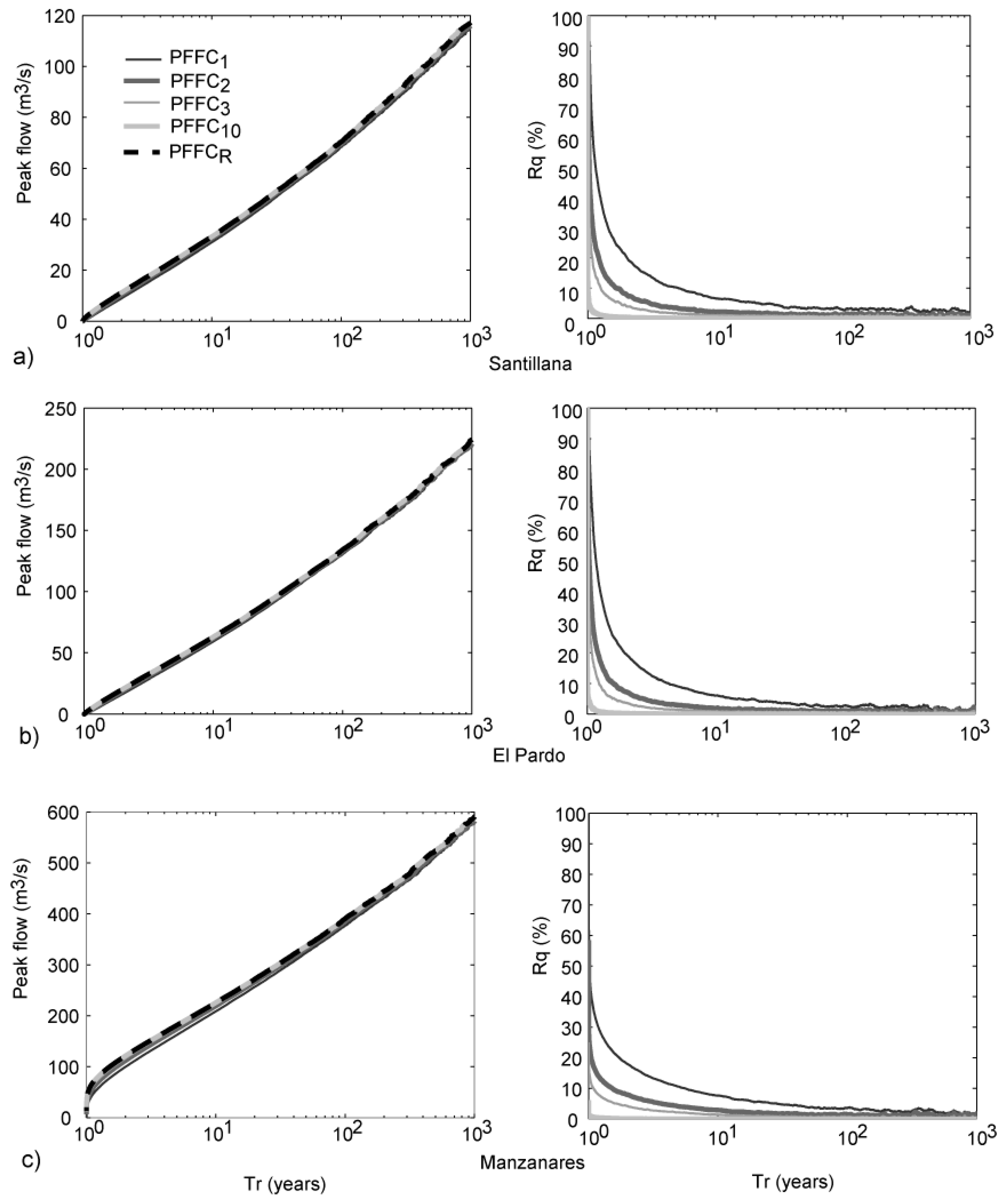
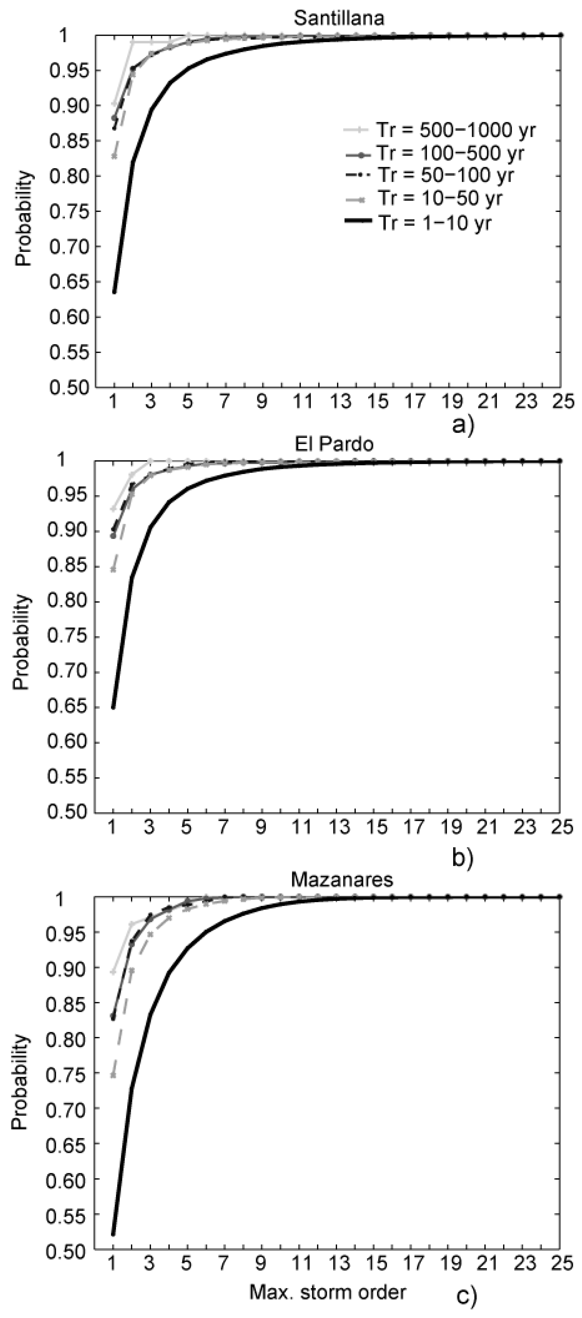
3.2. FFCs Estimation and Effect of Considering Different Number of Storms Each Year

As mentioned, for each year we sorted the identified storms from the highest to the lowest according to three criteria: (a) the total rainfall depth; (b) the storm duration; and (c) the mean storm intensity. Then, we performed the rainfall–runoff simulations. Figure 7 shows that for all analyzed cases the criterion of total rainfall depth was the most relevant one; that is, lower storm orders are needed for obtaining the annual maximum peak flow. For all case studies, more than 60% of the annual maximum peak flows were generated considering the largest storm (order 1) with the criterion of the maximum total rainfall depth each year, more than 80% considering storms of order 1 and 2 and more than 90% considering storms of order 1, 2 and 3. Considering the criterion of storm durations, the percentages decreased down to 30%, 50% and 60%, respectively, and applying the mean intensity criterion the percentages were lower than 10%, 20% and 30%, respectively. Flores-Montoya et al. [55] carried out a similar analysis by classifying the storms according to the mentioned three criteria. They transformed the storms into runoff by a distributed rainfall–runoff event model obtaining the corresponding hydrographs and the annual maximum peak flows. Results agree with this study. This suggests that the suitability of the criterion of the maximum total depth has a low dependence on the rainfall–runoff model utilized.
As mentioned, we utilized the hourly event-based hydrologic model for Manzanares basin developed by Sordo-Ward et al. [27]. They showed a good agreement for the comparison of the peak flow frequency curve obtained from observed and simulated data, mainly for high return periods (100 ≤ Tr ≤ 10,000 years). Figure 8 compares the observed peak flow and corresponding simulated peak flow (hourly time-step simulation) at the outlet of Manzanares basin, from six storm events with simultaneously recorded hourly rainfall and flow data. Results show an overall good agreement.
Different FFCs were estimated according to the proposed methodology. As mentioned, the largest storm each year (according to the annual maximum total rainfall depth) was named as storm of order 1, the second largest storm each year was named as storm of order 2 and so on until a maximum of 25 storms selected per year. First, using only the largest storm of each year, a FFC was calculated (FFC1). Second, we calculated the FFC2 considering the two largest storms of each year (order 1 + order 2). This was repeated until a maximum of 25 storms were selected. The FFC calculated with all 25 storm events was considered the reference FFC (FFCR). The procedure was repeated for the three analyzed basins. Figure 9 (left) shows the FFCs obtained for each basin and different storm orders. Results evidenced a general similarity among the different FFCs for all cases. However, a deeper analysis showed that the behavior of the FFCs changed according to the Tr of the peak flow considered. In order to quantify it, Figure 9 (right) shows the ratio between de FFCs for different cumulated orders (order 1, 1 + 2, 1 + 2 + 3, …, 1 + 2 + 3 + … 24) and the reference FFCR (order 1 + 2 + 3 …. + 25). The fewer storms considered per year and/or the lower the Tr analyzed, the lower the ratio becomes. The difference between the FFC1 and the FFCR was higher than 6% (up to 22%) for Tr ≤ 10 years. For 10 ≤ Tr ≤ 1000 years, the difference stabilized between 2% and 6%. The difference between the FFC2 and the FFCR was around 3%–30% for Tr ≤ 10 years. For 10 ≤ Tr ≤ 500 years, the difference stabilized between 1.5% and 3% and, for 500 ≤ Tr ≤ 1000 years, it decreased to around 1%–2%. The difference was lower than 5% for Tr ≤ 10 years for the comparison between the FFC4 and FFCR. For 10 ≤ Tr ≤ 1000 years, the difference stabilized around 1%–2%. In all cases, the higher the basin area, the lower the difference. In addition, the difference when comparing the FFCs among them (i.e., FFC1, FFC2, …, FFC24) decreased significantly when increasing the Tr analyzed. For example, for 100 ≤ Tr ≤ 1000, the difference between FFC1 and FFC4 was around 5%. We observed that for FFC3 and higher and for Tr ≥ 50 years, the difference among them were lower than 3%. As it regards the effect of basin area, the behavior of the FFCs and the ratio analysis for the three basins were found to be similar.
In addition, the relationship among the different storm orders, the peak flow generated for each storm and the Tr associated was analyzed. Figure 10 shows the probability for a storm of a specific order to generate the maximum peak flow of a year and the Tr range obtained for each storm order. When considering only the largest storm each year, the maximum peak flow of a year was obtained for 55% to 67% of the 100,000 analyzed years (depending on the considered basin, Figure 10). Thus, in order to guarantee obtaining the storm that generates the maximum annual peak flow each year, more than one storm each year should be considered. Results showed that although first order storms produced the maximum peak flow of a year only for 55% to 67% of the 100,000 analyzed years, the value of the maximum peak-flow quantiles obtained for the first order storms differed only between 5% and 8% (for Tr ≥ 10 years) with respect to the values obtained with the FFCR that considers all 25 storms every year (Figure 9).
Moreover, Figure 10 shows that there is a relationship between the maximum peak flow for each year and the order of the associated storm; that is, the maximum annual peak flows were generated by low order storms (e.g., the cumulated third order storm resulted into the maximum annual peak flow in the 85%–92% of the years depending on the analyzed basin).
Figure 11 shows the different case studies and different Tr ranges, and the cumulated probability for accounting the maximum peak flow in a specific year by considering different cumulated storm orders. As an example, Table 2 shows, for the case studies analyzed, the maximum order of storms to be extracted to obtain 95% and 99% probability of including the maximum peak flow in a specific year. For 95% probability and Tr ≤ 10 years, the four to six largest storms each year need to be extracted, whereas only the two largest storms need to be extracted for Tr ≥ 50 years. For the analyzed cases, it is shown that, for Tr ≥ 10 years, the maximum storm order to be extracted for achieving the maximum peak flow for a specific year had low dependence on the Tr considered (Figure 11 and Table 2). We found a basin area scale effect: the behavior of the Santillana and the Pardo sub-basins was similar but different to that of the Manzanares basin. Such difference increased for low maximum storm orders (3 or lower). The above suggests that for larger basins the temporal distribution of the storms and the runoff and propagation processes became relevant in order to obtain (or not) hydrographs with the maximum peak flow; however, for smaller basins, the correlation between the storm volume and the peak flow is higher.
Finally, we considered the 100,000 maximum annual peak-flow values with their corresponding storm order. Figure 12 shows the maximum storm order required to include the maximum peak flow for a specific year for different probabilities. The 95% probability was reached with between four and six maximum storm orders (depending on the case study) and 99% probability required an order of 10. As expected, these results are strongly conditioned by the low Tr floods as they are much more numerous than the higher Tr ones.

3.3. Joint Analysis of Maximum Annual Peak Flow and Hydrograph Volume

Given the relevance of knowing the peak flow and the hydrograph volume for the hydrologic design of some infrastructures, a joint analysis for both variables was performed for the Manzanares basin. Figure 13a shows the maximum storm order required to include simultaneously the event of maximum annual peak flow and hydrograph volume for different cumulated frequencies and Tr ranges. In this case, the Tr was calculated from the maximum peak flow each year. Results show that for 500 ≤ Tr ≤ 1000 years and by extracting only the three largest storms per year, there was 95% probability of achieving the hydrograph with the highest peak flow and volume. For cumulated orders higher than six, the cumulated frequency remained 98%, which means that there is a 2% probability of not obtaining the hydrograph with the maximum peak flow and hydrograph volume for a given year. However, for 1 ≤ Tr ≤ 10 years and by considering the three largest storms per year, we had a 59% probability (62% for storms characterized by ≤6 order) to include the hydrograph with the highest peak flow and volume and, similarly, a 41% probability of not achieving a hydrograph with the maximum peak flow and hydrograph volume. The above suggests that, for lower Tr, the temporal distribution of the storms becomes relevant for getting (or not) hydrographs with the maximum peak flow and hydrograph volume; however, for higher Tr, the storm volume appears as the key variable. Figure 13b is similar to Figure 13a but the Tr was calculated from the maximum hydrograph volume each year. Although the results are similar for 1 ≤ Tr ≤ 10 years, they differ for higher Trs. For 100 ≤ Tr ≤ 1000 years, the annual largest storm had a 98% probability of achieving the hydrograph with the maximum peak flow and hydrograph volume, which means, the storm volume for high Tr is more important for the determination of the highest hydrograph volumes than the maximum peak-flow hydrographs.

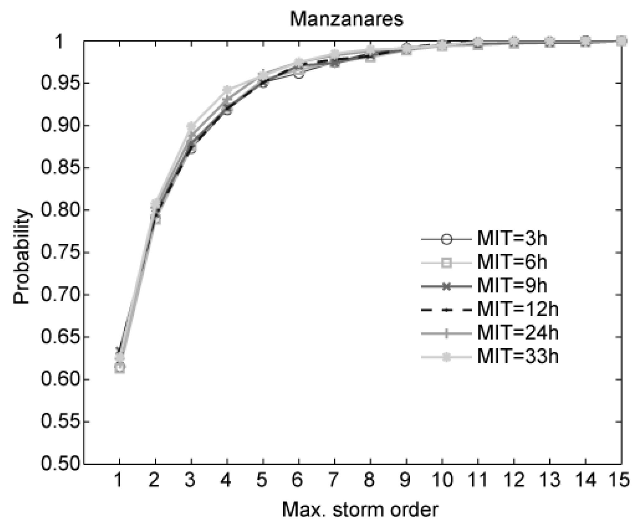
3.4. Sensitivity Analysis of Inter-Event Time Determination

For this study, we assumed that the minimum inter-event time (MIT) of no rain between two storm events to be considered as independent events was determined by applying the exponential method [47], with a value of 33 h. However, other authors used smaller values of MIT [44,54]. In this section, we performed a sensitivity analysis of the effect of the MIT on the maximum order of the storms that generate the maximum peak flow each year. We performed this analysis for the Manzanares basin and a time-series of 1000 years. We analyzed different MIT ranging between 3 and 33 h according to Dunkerley [43]. Figure 14 presents the maximum storm order required for including the maximum peak flow in a specific year with different probabilities and MITs. Results show that the general behavior for the different inter-event times analyzed was similar, achieving differences lower than 3% between the shortest (3 h) and the longest (33 h) inter-event times considered. Short inter-event time periods imply longer storm durations and larger storm volumes triggering higher peak flows and then higher values of accumulated frequency for smaller inter-event times.

4. Conclusions

This study shows the feasibility of the estimation of the peak-flow frequency curves for high return periods based on a stochastic rainfall model coupled with an event-based rainfall–runoff model. The study provides a methodology for the estimation of the minimum number of storms to be considered according to the return period of interest. The obtained results and conclusions are restricted to the selected study basins. Despite this, the study clearly shows the influence of the number of storms considered each year on the estimation of the flood frequency curve. Moreover, the proposed methodology simulates the rainfall event for each sub-basin as spatially correlated, and simultaneously the defined storms have different associated return period, total depths, start times, durations and temporal patterns. Specifically:
  • The degree of alignment between the calculated flood frequency curves and the reference flood frequency curve depends on the return period of the peak flow considered.
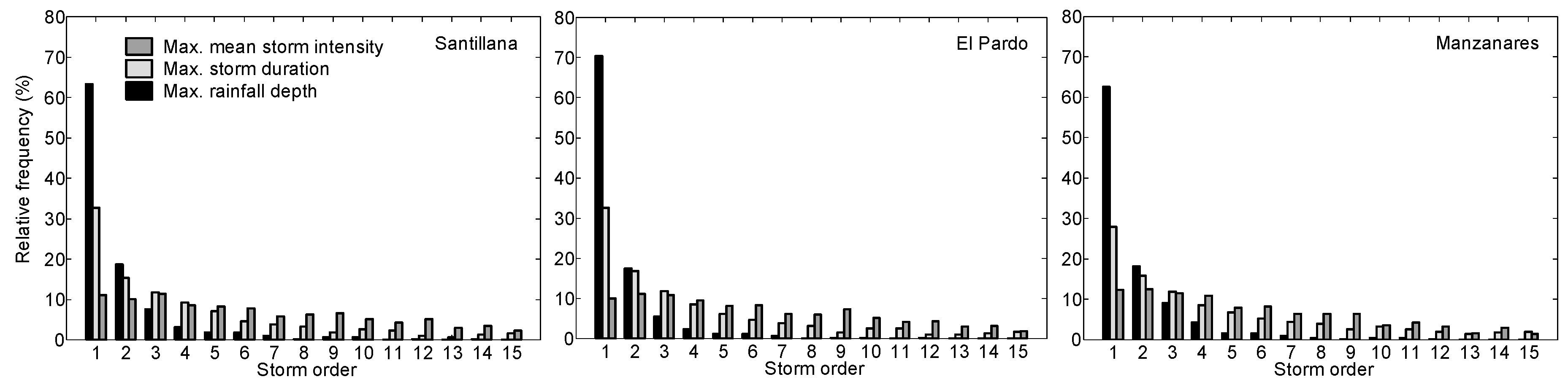
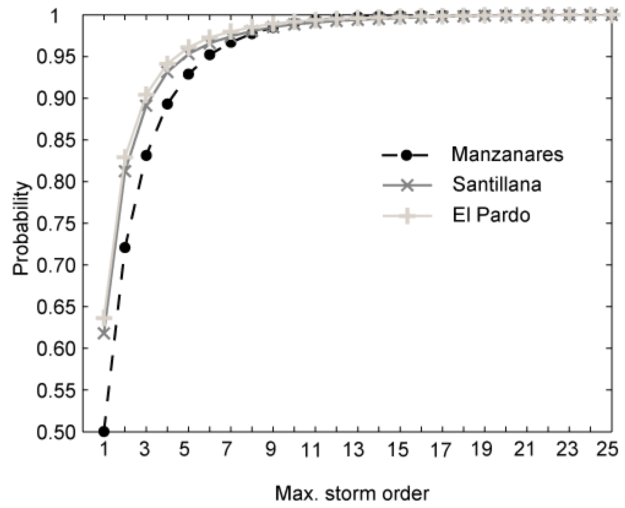
  • Considering the criterion of the total rainfall depth to define when one storm is larger than another, a strong correlation was found between this criterion and the corresponding peak flow. Considering the three largest storms each year, the probability of achieving the maximum annual peak flow ranges between 83% and 92% depending on the analyzed basin.
  • The flood frequency curve for high return period (50 ≤ return period ≤ 1000 years) generated by considering the three largest storms each year can be estimated with a difference lower than 3% regarding the reference flood frequency curve.
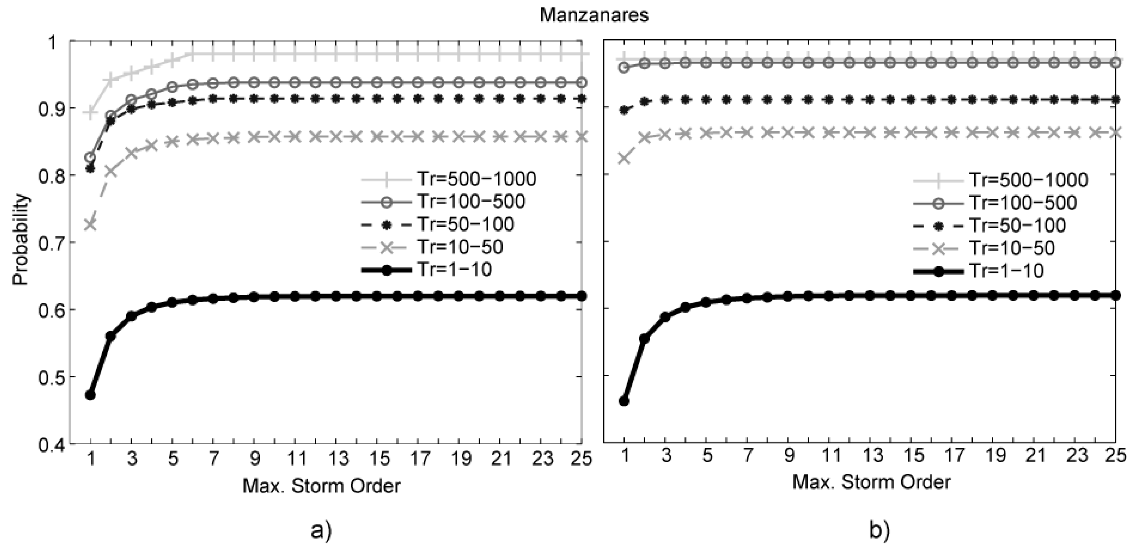
  • By using the largest storm each year, for return periods higher than 10 years, the derived flood frequency curve determines which storms of order 1 show a difference lower than 10% regarding the reference flood frequency curve (considering all the identified storms).
  • Basins with larger catchment areas would require more annual largest storms than in smaller basins in order to achieve the maximum peak flow each year.
  • Considering the three largest storms each year, the probability of achieving simultaneously a hydrograph with the maximum annual peak flow and the maximum annual volume for a return period higher than 100 years is 94%, the return period being calculated from the maximum annual peak flows series. If we calculated the return period from the maximum annual hydrograph volume series, the probability would increase to 98%.
  • The inter-storm time shows low influence on determining the minimum number of largest storms to be considered for achieving the maximum annually peak flow. Considering a wide range of inter-storm time (3 to 33 h) for the identification of storm events, the difference of the probability of including the maximum peak flow for a specific number of storms considered each year is lower than 3% in all cases.

Acknowledgments

The study was made possible by the funds from Fundación José Entrecanales Ibarra in the framework of the Program “Support program for young professors for doing international stays” and to the National Meteorological Agency (AEMET) for the rainfall data.

Author Contributions

Alvaro Sordo-Ward led the conceptual and methodological design of the manuscript, and he also participated in the analysis and discussion of results and paper writing; Paola Bianucci conducted the numerical experiments and participated in the analysis and discussion of results and paper writing; Luis Garrote contributed to the general idea of the research and he participated in the analysis and discussion of results and paper writing; and Alfredo Granados helped in the analysis and discussion of results, wrote the English edition of the manuscript and proposed improved figures for a better understanding of the results.

Conflicts of Interest

The authors declare no conflict of interest.

Abbreviations

The following abbreviations are used in this manuscript:
CFCumulative frequency distribution
CVCoefficient of variation
FFCiPeak-flow frequency curve considering the i largest storms of each year
FFCRReference peak-flow frequency curve considering a maximum of 25 largest storms of each year
IDFIntensity–Duration–Frequency curves
MITMinimum inter-event time (hours)
NSNash–Sutcliffe coefficient
RFRelative frequency distribution
RqRatio between the FFCs for different maximum storm orders and the reference FFCR
TrReturn period (years)

References

  1. Smith, A.; Sampson, C.; Bates, P. Regional flood frequency analysis at the global scale. Water Resour. Res. 2015, 51, 539–553. [Google Scholar]
  2. Botto, A.; Ganora, D.; Laio, F.; Claps, P. Uncertainty compliant design flood estimation. Water Resour. Res. 2014, 50, 4242–4253. [Google Scholar] [CrossRef]
  3. Nguyen, C.; Gaume, E.; Payrastre, O. Regional flood frequency analyses involving extraordinary flood events at ungauged sites: Further developments and validations. J. Hydrol. 2014, 508, 385–396. [Google Scholar] [CrossRef]
  4. Laio, F.; Ganora, D.; Claps, P.; Galeati, G. Spatially smooth regional estimation of the flood frequency curve (with uncertainty). J. Hydrol. 2011, 408, 67–77. [Google Scholar] [CrossRef]
  5. Merz, R.; Blöschl, G. Flood frequency hydrology: 1. Temporal, spatial, and causal expansion of information. Water Resour. Res. 2008, 44. [Google Scholar] [CrossRef]
  6. Goñi, M.; López, J.J.; Gimena, F.N. Reservoir rainfall–runoff geomorphological model. I: Application and parameter analysis. Hydrol. Process. 2013, 27, 477–488. [Google Scholar] [CrossRef]
  7. Goñi, M.; López, J.J.; Gimena, F.N. Reservoir rainfall-runoff geomorphological model. II: Analysis, calibration and validation. Hydrol. Process. 2013, 27, 489–504. [Google Scholar] [CrossRef]
  8. Hadadin, N. Evaluation of several techniques for estimating storm water runoff in arid watersheds. Environ. Earth Sci. 2012, 69, 1773–1782. [Google Scholar] [CrossRef]
  9. Beven, K.J. Rainfall-Runoff Modelling: The Primer, 2nd ed.; Wiley-Blackwell: Hoboken, NJ, USA, 2008; p. 488. [Google Scholar]
  10. Singh, V.P.; Frevert, D.K. Mathematical Models of Small Watershed Hydrology and Applications; Water Resources Publication: Highlands Ranch, CO, USA, 2002; p. 950. [Google Scholar]
  11. Singh, V.P.; Frevert, D.K. Mathematical Models of Large Watershed Hydrology; Water Resources Publication: Highlands Ranch, CO, USA, 2002; p. 891. [Google Scholar]
  12. Raines, T.; Valdés, J. Estimation of flood frequencies for ungaged catchments. J. Hydraul. Eng. 1993, 119, 1138–1154. [Google Scholar] [CrossRef]
  13. Hadadin, N. Modeling of Rainfall-Runoff Relationship in Semi-Arid Watershed in the Central Region of Jordan. Jordan J. Civ. Eng. 2016, 10, 209–218. [Google Scholar] [CrossRef]
  14. Blazkova, S.; Beven, K. A limits of acceptability approach to model evaluation and uncertainty estimation in flood frequency estimation by continuous simulation: Skalka catchment, Czech Republic. Water Resour. Res. 2009, 45. [Google Scholar] [CrossRef]
  15. Samuel, J.M.; Sivapalan, M. Effects of multiscale rainfall variability on flood frequency: Comparative multisite analysis of dominant runoff processes. Water Resour. Res. 2008, 44. [Google Scholar] [CrossRef]
  16. Aronica, G.; Candela, A. Derivation of flood frequency curves in poorly gauged Mediterranean catchments using a simple stochastic hydrological rainfall-runoff model. J. Hydrol. 2007, 347, 132–142. [Google Scholar] [CrossRef]
  17. Arnaud, P.; Lavabre, J. Coupled rainfall model and discharge model for flood frequency estimation. Water Resour. Res. 2002, 38. [Google Scholar] [CrossRef]
  18. Loukas, A. Flood frequency estimation by a derived distribution procedure. J. Hydrol. 2002, 255, 69–89. [Google Scholar] [CrossRef]
  19. Rahman, A.; Weinmann, P.E.; Hoang, T.M.T.; Laurenson, E.M. Monte Carlo simulation of flood frequency curves from rainfall. J. Hydrol. 2002, 256, 196–210. [Google Scholar] [CrossRef]
  20. Wagener, T.; Wheater, H.S.; Gupta, H.V. Rainfall-Runoff Modelling in Gauged and Ungauged Catchments; Imperial College Press: London, UK, 2004; p. 332. [Google Scholar]
  21. Berthet, L.; Andréassian, V.; Perrin, C.; Javelle, P. How crucial is it to account for the antecedent moisture conditions in flood forecasting? Comparison of event-based and continuous approaches on 178 catchments. Hydrol. Earth Syst. Sci. 2009, 13, 819–831. [Google Scholar] [CrossRef]
  22. Sivapalan, M.; Wood, E.; Beven, K. On hydrologic similarity: 3. A dimensionless flood frequency model using a generalized geomorphic unit hydrograph and partial area runoff generation. Water Resour. Res. 1990, 26, 43–58. [Google Scholar] [CrossRef]
  23. Natural Environment Research Council (NERC). Flood Studies Report; Natural Environment Research Council (NERC): London, UK, 1975. [Google Scholar]
  24. Flores-Montoya, I.; Sordo-Ward, A.; Mediero, L.; Garrote, L. Fully stochastic distributed methodology for multivariate flood frequency analysis. Water 2016, 8. [Google Scholar] [CrossRef]
  25. De Michele, C.; Salvadori, G. On the derived flood frequency distribution: Analytical formulation and the influence of antecedent soil moisture condition. J. Hydrol. 2002, 262, 245–258. [Google Scholar] [CrossRef]
  26. Silveira, L.; Charbonier, F.; Genta, J. The antecedent soil moisture condition of the curve number procedure. Hydrol. Sci. J. 2000, 45, 3–12. [Google Scholar] [CrossRef]
  27. Sordo-Ward, A.; Bianucci, P.; Garrote, L.; Granados, A. How safe is hydrologic infrastructure design? Analysis of factors affecting extreme flood estimation. J. Hydrol. Eng. 2014, 19. [Google Scholar] [CrossRef]
  28. Viglione, A.; Blöschl, G. On the role of storm duration in the mapping of rainfall to flood return periods. Hydrol. Earth Syst. Sci. 2009, 13, 205–216. [Google Scholar] [CrossRef]
  29. Alfieri, L.; Laio, F.; Claps, P. A simulation experiment for optimal design hyetograph selection. Hydrol. Process. 2008, 22, 813–820. [Google Scholar] [CrossRef]
  30. Blazkova, S.; Beven, K. Flood frequency estimation by continuous simulation of subcatchment rainfalls and discharges with the aim of improving dam safety assessment in a large basin in the Czech Republic. J. Hydrol. 2004, 292, 153–172. [Google Scholar] [CrossRef]
  31. Bocchiola, D.; Rosso, R. Use of a derived distribution approach for extreme floods design: A case study in Italy. Adv. Water Resour. 2009, 32, 1284–1296. [Google Scholar] [CrossRef]
  32. Andres-Domenech, I.; Montanari, A.; Marco, J.B. Stochastic rainfall analysis for storm tank performance evaluation. Hydrol. Earth Syst. Sci. 2010, 14, 1221–1232. [Google Scholar] [CrossRef]
  33. Arnaud, P.; Fine, J.; Lavabre, J. An hourly rainfall generation model applicable to all types of climate. Atmos. Res. 2007, 85, 230–242. [Google Scholar] [CrossRef]
  34. Wilks, D.; Wilby, R. The weather generation game: A stochastic weather models. Prog. Phys. Geogr. 1999, 23, 329–357. [Google Scholar] [CrossRef]
  35. Candela, A.; Brigandì, G.; Aronica, G.T. Estimation of synthetic flood design hydrographs using a distributed rainfall–runoff model coupled with a copula-based single storm rainfall generator. Nat. Hazards Earth Syst. Sci. 2014, 14, 1819–1833. [Google Scholar] [CrossRef] [Green Version]
  36. Vandenberghe, S.; Verhoest, N.E.C.; Buyse, E.; De Baets, B. A stochastic design rainfall generator based on copulas and mass curves. Hydrol. Earth Syst. Sci. 2010, 14, 2429–2442. [Google Scholar] [CrossRef]
  37. Kao, S.C.; Govindaraju, R.S. Trivariate statistical analysis of extreme rainfall events via the Plackett family of copulas. Water Resour. Res. 2008, 44. [Google Scholar] [CrossRef]
  38. Grimaldi, S.; Serinaldi, F. Design hyetograph analysis with 3-copula function. J. Sci. Hydrol. 2006, 51, 223–238. [Google Scholar] [CrossRef]
  39. Burton, A.; Fowler, H.J.; Kilsby, C.G.; O’Connell, P.E. A stochastic model for the spatial-temporal simulation of nonhomogeneous rainfall occurrence and amounts. Water Resour. Res. 2010, 46. [Google Scholar] [CrossRef]
  40. Burton, A.; Kilsby, C.G.; Fowler, H.J.; Cowpertwait, P.S.P.; O’Connell, P.E. RainSim: A spatial–temporal stochastic rainfall modelling system. Environ. Model. Softw. 2008, 23, 1356–1369. [Google Scholar] [CrossRef]
  41. Salsón, S.; García-Bartual, R. A space-time rainfall generator for highly convective Mediterranean rainstorms. Nat. Hazards Earth Syst. Sci. 2003, 3, 103–114. [Google Scholar] [CrossRef]
  42. Cowpertwait, P.; Kilsby, C.; O’Connell, P. A space-time Neyman-Scott model of rainfall: Empirical analysis of extremes. Water Resour. Res. 2002, 38. [Google Scholar] [CrossRef]
  43. Dunkerley, D. Identifying individual rain events from pluviograph records: A review with analysis of data from an Australian dryland site. J. Hydrol. Process. 2008, 22, 5024–5036. [Google Scholar] [CrossRef]
  44. Aryal, R.K.; Furumai, H.; Nakajima, F.; Jinadasa, H.K.P.K. The role of inter-event time definition and recovery of initial/depression loss for the accuracy in quantitative simulations of highway runoff. Urban Water J. 2007, 4, 53–58. [Google Scholar] [CrossRef]
  45. Bonta, J.V.; Rao, A.R. Factors affecting the identification of independent storm events. J. Hydrol. 1988, 98, 275–293. [Google Scholar] [CrossRef]
  46. Restrepo-Posada, P.J.; Eagleson, P.S. Identification of inde-pendent rainstorms. J. Hydrol. 1982, 55, 303–319. [Google Scholar] [CrossRef]
  47. Duan, Q.; Soorooshian, S.; Gupta, V. Effective and efficient global optimization for conceptual rainfall-runoff models. Water Resour. Res. 1992, 28, 1015–1031. [Google Scholar] [CrossRef]
  48. Campo, M.A.; Sordo, A.; González-Zeas, D.; Cirauqui, D.; Garrote, L.; López, J. Application of a stochastic rainfall model in flood risk assessment. Geophys. Res. Abstr. 2009, 11. [Google Scholar] [CrossRef]
  49. Sordo-Ward, A.; Garrote, L.; Bejarano, M.D.; Castillo, L.G. Extreme flood abatement in large dams with gate-controlled spillways. J. Hydrol. 2013, 498, 113–123. [Google Scholar] [CrossRef]
  50. Sordo-Ward, A.; Garrote, L.; Martín-Carrasco, F.; Bejarano, M.D. Extreme flood abatement in large dams with fixed-crest spillways. J. Hydrol. 2012, 466–467, 60–72. [Google Scholar] [CrossRef] [Green Version]
  51. Bianucci, P.; Sordo-Ward, A.; Moralo, J.; Garrote, L. Probabilistic-Multi objective Comparison of User-Defined Operating Rules. Case Study: Hydropower Dam in Spain. Water 2015, 7, 956–974. [Google Scholar] [CrossRef]
  52. United States Soil Conservation Service. National Engineering Handbook, Section 4: Hydrology; U.S. Department of Agriculture: Washington, DC, USA, 1972; p. 127.
  53. McCarthy, G.T. The Unit Hydrograph and Flood Routing; US Army Corps of Engineers: Providence, RI, USA, 1939. [Google Scholar]
  54. Nash, J.E.; Sutcliffe, J.V. River flow forecasting through conceptual models, Part I—A discussion of principles. J. Hydrol. 1970, 10, 282–290. [Google Scholar] [CrossRef]
  55. Flores-Montoya, I.; Requena, A.; Sordo-Ward, A.; Mediero, L.; Garrote, L. Deriving bivariate flood frequency distributions for dam safety evaluation. In Proceedings of the 8th International Conference of European Water Resources Association (EWRA): Water Resources Management in an Interdisciplinary and Changing Context, Porto, Portugal, 26–29 June 2013.
Figure 1. General methodology scheme.
Water 08 00335 g001
Figure 2. Methodological scheme for the determination of the storm event durations and the storm event definition for each sub-basin: (a) independent storm identification and extraction from the mean hourly time-series for the entire basin and period of analysis; (b) mean storm event for each defined sub-basin from the identified event periods.
Water 08 00335 g002
Figure 3. Location of the case studies. Black circles show the basin outlets and the dots characterized by an alphanumeric code representing the rainfall gauge stations considered in this study.
Water 08 00335 g003
Figure 4. Validation of the spatial–temporal stochastic rainfall model. Dots represent the annual maxima of the daily rainfall frequency curve from observed data. Grey lines represent frequency curves of annual maxima of daily rainfall from 60 simulated series of 100 years.
Water 08 00335 g004
Figure 5. Comparison of the Intensity-Duration-Frequency curves (IDF) obtained from observed data (station ID-3195, 5-min time-step) and from the results of the RainSimV3 model (hourly time-step).
Water 08 00335 g005
Figure 6. Main characteristics of the entire set of storm events and the set of maximum annual rain depth storm events extracted from the continuous spatially-averaged rainfall series: (a) total rainfall depth in mm; (b) storm duration in hours; (c) storm mean intensity in mm/hours; and (d) inter-event time in hours. Dotted lines represent the cumulative frequency distributions of non-exceedance for the entire set and crossed dashed lines do the same for the subset of the maximum annual rain depth storms. Dark bars show the relative frequency for the entire set and light bars do it for the subset of the maximum annual rain depth storms.
Water 08 00335 g006
Figure 7. Comparison among the three criteria for identifying the highest annual storms. Percentage of occurrence that a storm of a specific order generates the annual maximum peak flow: (Left) Santillana sub-basin; (Centre) El Pardo sub-basin; and (Right) Manzanares basin.
Water 08 00335 g007
Figure 8. Comparison among the observed peak flow and corresponding simulated peak flow (hourly time-step) at the outlet of Manzanares basin.
Water 08 00335 g008
Figure 9. (Left) FFCs obtained for each basin and different storm orders; and (Right) ratio between the FFCs for different maximum storm orders and the reference FFCR: (a) Santillana sub-basin; (b) The Pardo sub-basin; and (c) Manzanares basin. Thin black lines show the results (the FFC and ratio) for the largest rainfall depth each year, the wide black lines considering the two largest rainfall depths each year, the thin grey lines the three largest rainfall depths each year, the wide grey lines the 10 largest rainfall depths rainfall each year and the dashed black lines shows the reference FFC.
Water 08 00335 g009
Figure 10. For each analyzed basin, the figure shows the storm order that corresponds to every Tr, represented as grey dots: (a) Santillana sub-basin; (b) The Pardo sub-basin; (c) Manzanares basin. The numbers on the right represent the probability that a storm of a specific order generates the maximum peak flow of given a year.
Water 08 00335 g010
Figure 11. For each analyzed basin, the plot shows the probability to generate the maximum peak flow of a year simulating only storms of a specific order or lower: (a) Santillana sub-basin; (b) The Pardo sub-basin; (c) Manzanares basin. The black lines represent the maximum annual peak-flows with 1 ≤ Tr < 10 years, the dark dashed grey lines for 10 ≤ Tr < 50 years, the thin dashed black lines for 50 ≤ Tr < 100 years, the dark grey lines for 100 ≤ Tr < 500 years and the light grey lines for 500 ≤ Tr < 1000 years.
Water 08 00335 g011
Figure 12. Maximum storm order required to include the maximum peak flow each year for different probabilities. Dot and dashed line corresponds to the Santillana sub-basin, dotted line to the Pardo sub-basin and dashed line to the Manzanares basin.
Water 08 00335 g012
Figure 13. Maximum storm order required to achieve, simultaneously, the event of maximum annual peak flow and hydrograph volume for different cumulated probabilities and Tr ranges. (a) Tr calculated from the maximum peak flow each year (Manzanares); (b) Tr calculated from the maximum hydrograph volume each year (Manzanares). The black lines represent the maximum annual peak flows with 1 ≤ Tr < 10 years, the dark dashed grey lines for 10 ≤ Tr < 50 years, the thin dashed black lines for 50 ≤ Tr < 100 years, the dark grey lines for 100 ≤ Tr < 500 years and the light grey lines for 500 ≤ Tr < 1000 years.
Water 08 00335 g013
Figure 14. Maximum storm order required to achieve the maximum peak flow each year for different probabilities and MITs (Manzanares basin). The line with a circle corresponds to MIT 3 h, the line with the rectangle to MIT 6 h, the dark line with the cross to MIT 9 h, the dashed line to MIT 12 h, the grey line with a cross to MIT 24 h and the light grey line with a solid circle correspond to MIT 33 h.
Water 08 00335 g014
Table 1. Characterization of the basins considered in this study.
NameArea (km2)N° Sub-BasinsSub-Basin Area (km2)
AverageRange
Santillana2115426.4/89
Pardo4957716.4/196
Manzanares129414926.4/255
Table 2. Maximum storm order required to obtain 95% and 99% probability of achieving the maximum peak flow for a specific year.
Probability (%)Tr (Years)Maximum Storm Order to Be Considered
SantillanaPardoManzanares
95/991 ≤ Tr < 105/114/96/10
95/9910 ≤ Tr < 502/52/53/6
95/9950 ≤ Tr ≤ 1002/52/53/6
95/99100 ≤ Tr ≤ 5002/52/52/5
95/99500 ≤ Tr ≤ 10001/22/32/5

