Hydrological Modeling of the Upper Indus Basin: A Case Study from a High-Altitude Glacierized Catchment Hunza

Abstract

The Soil and Water Assessment Tool (SWAT) model combined with a temperature index and elevation band algorithm was applied to the Hunza watershed, where snow and glacier-melt are the major contributor to river flow. This study’s uniqueness is its use of a snow melt algorithm (temperature index with elevation bands) combined with the SWAT, applied to evaluate the performance of the SWAT model in the highly snow and glacier covered watershed of the Upper Indus Basin in response to climate change on future streamflow volume at the outlet of the Hunza watershed, and its contribution to the Indus River System in both space and time, despite its limitation; it is not designed to cover the watershed of heterogeneous mountains. The model was calibrated for the years 1998–2004 and validated for the years 2008–2010. The model performance is evaluated using the four recommended statistical coefficients with uncertainty analysis (p-factor and r-factor). Simulations generated good calibration and validation results for the daily flow gauge. The model efficiency was evaluated, and a strong relationship was observed between the simulated and observed flows. The model results give a coefficient of determination (R²) of 0.82 and a Nash–Sutcliffe Efficiency index (NS) of 0.80 for the daily flow with values of p-factor (79%) and r-factor (76%). The SWAT model was also used to evaluate climate change impact on hydrological regimes, the target watershed with three GCMs (General Circulation Model) of the IPCC fifth report for 2030–2059 and 2070–2099, using 1980–2010 as the control period. Overall, temperature (1.39 °C to 6.58 °C) and precipitation (31%) indicated increased variability at the end of the century with increasing river flow (5%–10%); in particular, the analysis showed smaller absolute changes in the hydrology of the study area towards the end of the century. The results revealed that the calibrated model was more sensitive towards temperature and precipitation, snow-melt parameters and Curve Number (CN2). The SWAT results also provided reliable information for the daily runoff from the sub-basin watersheds responding to changing climatic conditions. SWAT can thus be used to devise effective strategies for future sustainable water management in the region, while combating vulnerabilities against floods and water storage in downstream water reservoirs such as the Diamer-Basha dam.

1. Introduction

Mountains play an important role in supplying water for downstream areas. The Himalayan Mountains are the source of eight major river systems, including Brahmaputra, Ganges, Indus, Irrawaddy, Mekong, Salween, Yangtze and Yellow River. About one-sixth of the global population depends on these freshwater sources i.e., glacier, ice and snow [1], which provide a lifeline for the people who inhabit the downstream areas [2]. Snow and glaciers in the Hindu Kush-Himalayan (HKH) mountains region also act as natural water reservoirs that constantly feed the Indus River and its tributaries [2]. Protecting these water resources is an emerging global challenge. Different models ranging from normal temperature-index-based algorithms to complex algorithms have been used to predict snow and glacier melting processes in the region [3] where snow and glacier melt provides stream flow for the Indus river system. Pakistan’s northern mountainous part, known as Gilgit-Baltistan (GB) with a varying elevation (2000 m to 8611 m above sea level) and unique glacier and snow cover dynamics, offers exclusive opportunities and challenges for researchers to better understand the hydrological processes occurring in the region.

Agriculture is the back bone of the Pakistan economy which is mainly dependent on the world’s largest integrated irrigation system, the Indus Basin Irrigation System (IBIS) [4]. Snow and glacier-melt and rainfall runoff from the northern watersheds of the Upper Indus Basin covering 2200 km² of the permanently glaciated area, potentially feed the Indus River system (IRS). Above 3500 m a.s.l. glaciers and permanent snowfields contribute 65% of the total annual flow to the Indus River System [5,6], as these glaciers are highly active with high flow rates (100–1000 m·year⁻¹) and often move through diverse climate zones [7].

Impacts of Climate change (CC) on regional hydrological regimes vary from basin to basin. Potential impacts on hydrological processes may include evapotranspiration, water temperature, streamflow volume, timing, frequency and magnitude of runoff, soil moisture, and severity of floods. These would impact other environmental variables such as sedimentation, plant growth and nutrient flow into water bodies [8]. The results of such hydrological changes would affect almost every aspect of human life i.e., agricultural productivity, water supply for urban and industrial use, power generation, wildlife and biotic ecosystems [8]. Climate change and global hydrological cycles play an important role in hydrological research as the results from these studies and their quantitative analysis (hydrological impact on climate change) are helpful for better understanding of potential hydrological risks for future water management planning. The model was also to conduct CC impact assessments at watershed scales (e.g., [9,10]).

The hydrological setting varies from region to region and the climate change was affected by the hydrological processes locally under the same climate conditions and scenarios [8]. Many studies have been conducted to calculate the snow and glacier melt and their hydrological processes on watershed or river basin scales in the Upper Indus Basin (UIB). Tahir et al. [2], Akhtar et al. [11], and others [12,13,14] have overlooked discussing glacier behavior on river basin scale [2,6], except [15]. Some studies have been carried out for the long-term prediction of streamflow based on future climate scenarios by adding the future monthly precipitation and temperature changes simulated by General Circulation Models (GCMs) to the baseline precipitation and temperature data [2] but none have adopted multi-objective or multi-variable calibration approaches, with the exception of [16], who used different parameters to analyze internal consistency simulation of glacier mass. Akhtar et al. [17] studied the effect of different model parameters using different input datasets. Most of the hydrological models applied on UIB are conceptual rather than physically [2,15,17] and spatially distributed [16,17]. Literature indicates that some of the hydrological regimes in UIB are extremely vulnerable to fast changing climatic conditions, particularly to changing temperature and precipitation patterns [2]. Therefore, it is important to study the local and regional level climatic patterns to better understand the impact of climate change on natural resources, as well as its adverse impact on human beings.

The majority of models that were used for UIB are simple lumped and temperature index based models, established by specific input datasets (statistical). Models rarely represented physical characteristics of the watershed. Hence, very little is known about the performance of the SWAT (Soil and Water Assessment Tool) model in a typical highly snow and glacier covered dry-temperate mountainous watershed, which provides a significant amount of water supply to the Indus River System. The SWAT model is capable of combining snow and glacier melt proportions with the water balance based on the temperature index by using the elevation bands and their areas. Elevation bands are a very important variable in hydro-meteorological parameters, including both temperature indices’ snow amounts. The SWAT allows the sub-basin to be split into 10 different elevation bands, and snow and glacier cover and their melting are simulated separately for each elevation band [18]. The SWAT evaluates evapotranspiration (ET) using various methods, such as Food and Agriculture Organization Penman–Monteith (FAO-PM), Hargreaves, and Priestley–Taylor. For this study, we used the Penman–Monteith method that was found to be suitable on the basis of initial model performance before calibration. Moreover, not a single study has been conducted yet using a complex, physical measurement based distributed hydrological model to assess the contribution of snow and glacier melts to IRS from this particular (Hunza) sub-basin.

Therefore, in order to fill this knowledge gap, the SWAT model was configured to simulate stream-flow (daily and monthly) of the Hunza river basin, in response to changing climatic scenarios (RCP5) with three different future climate change projection models. With fast changing economic and social conditions, demand for water supply is anticipated to become a more serious problem in the near future and therefore, it is important to understand possible impacts of climate change on stream flow, for sustainable water resource management in this region.

This study was therefore conducted to evaluate the performance of the SWAT model in a highly snow and glaciated watershed, in response to changing climate and its impact on streamflow volumes now, as well as in the long run, at the outlet of the Hunza watershed, and its contribution to the Indus River System, which may help the local water management authorities devise effective strategies for sustainable water management in the region.

2. Study Area

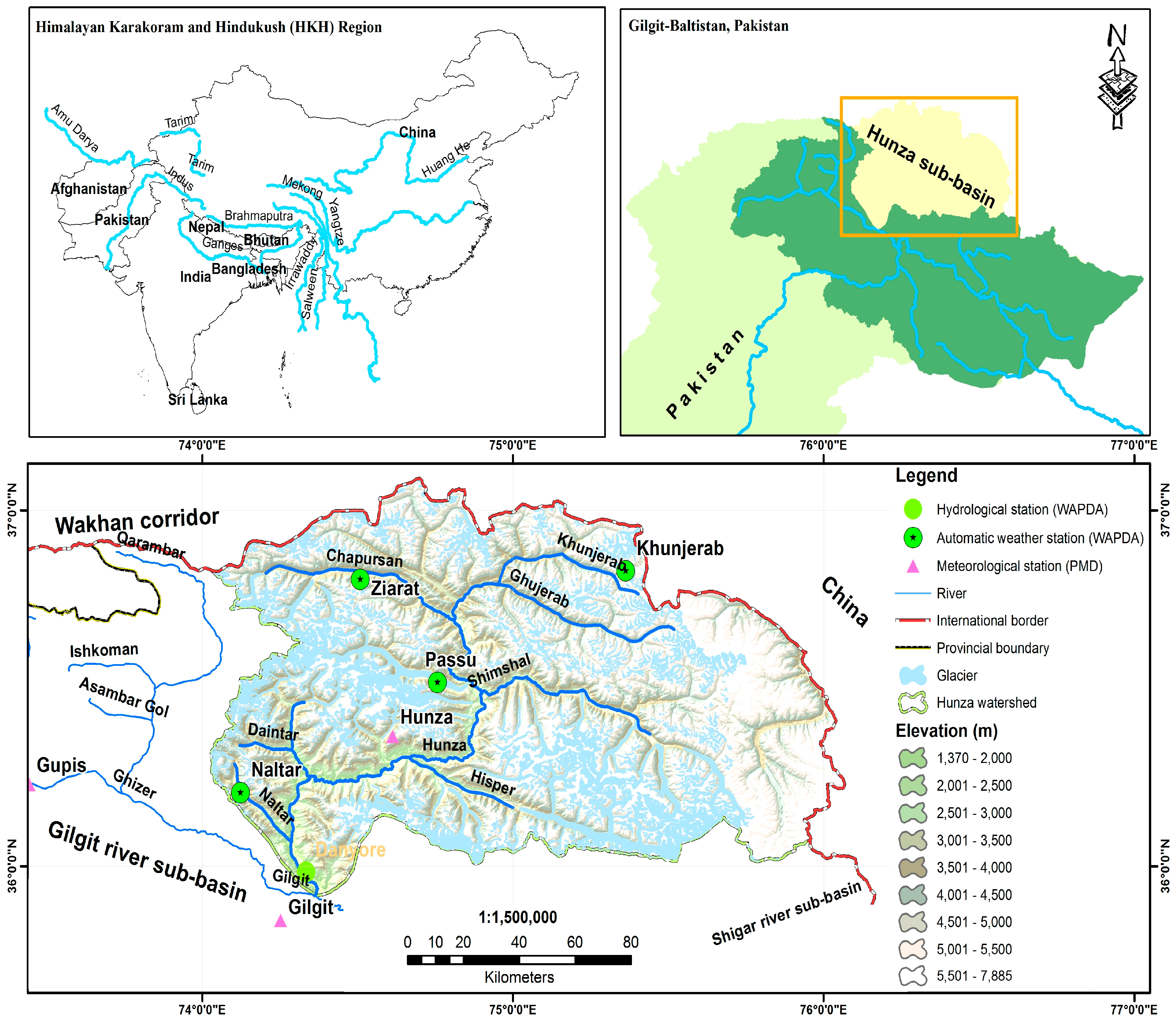
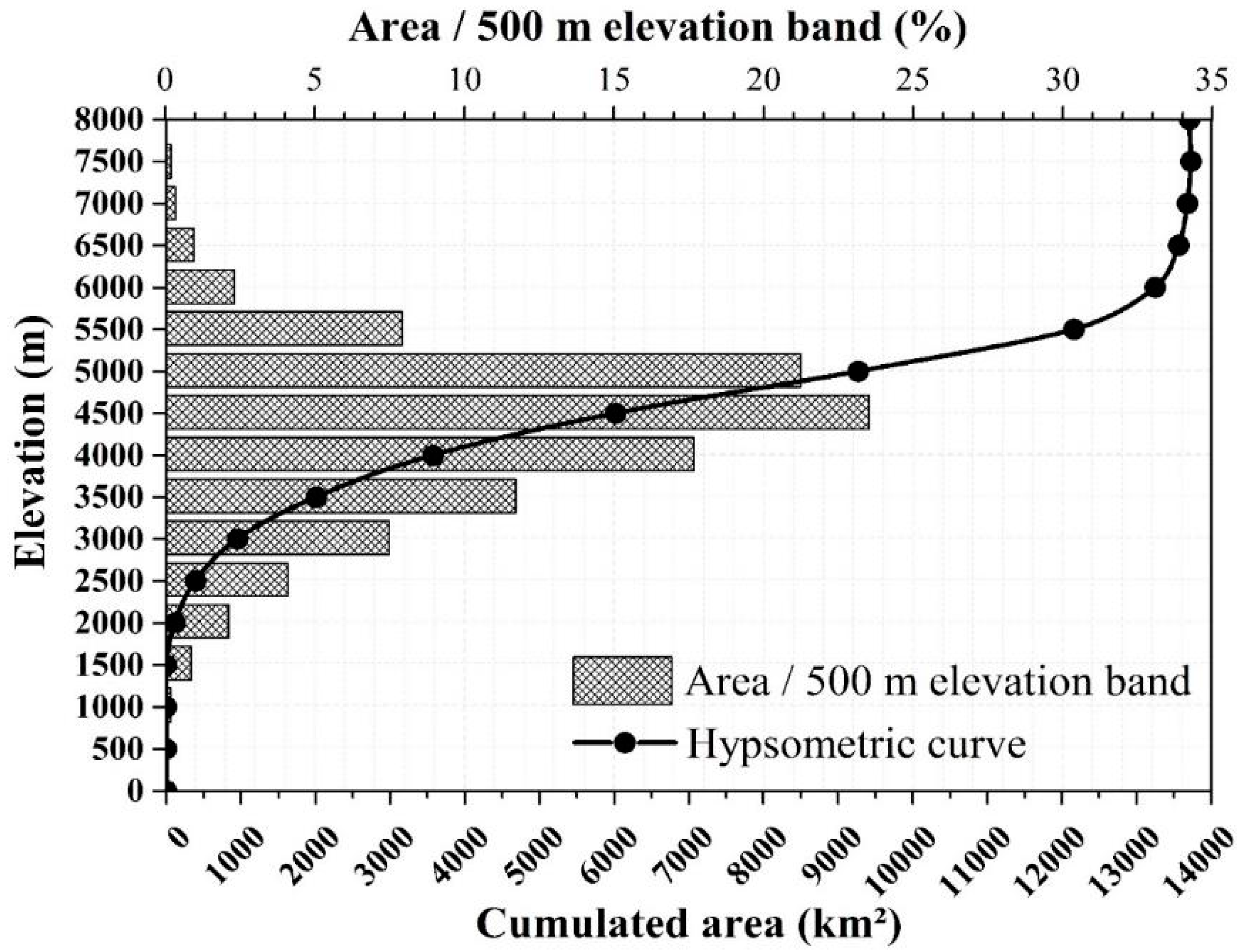
The Hunza watershed with an area of 13,567.23 km² is situated in the UIB area, Pakistan, in the north bordering with China and Afghanistan in the Karakoram mountain range (Figure 1). The main river (Hunza) is 231.76 km long with flow contributed to by fourteen small and medium tributary rivers, rivulets and streams, namely Danyore, Khunjerab, Verjerab, Chupurson, Misgar, Khudaabad, Khyber, Shimshal, Hisper, Hoper, Hassanabad, Rakaposhi, Chalt, and Naltar. The elevation curve of the watershed varies between 1394 m and 7885 m a.s.l. with a mean elevation of 4627 m (Figure 2). The lowest point is located at Danyore gauging station (1370 m a.s.l.) and the highest point is the Distaghil Sar (7885 m a.s.l.)—19th highest on the earth and seventh highest peak in Pakistan. About 50% of the total watershed area lies above 4700 m a.s.l. According to Surface water Hydrology Project of Water and Power Development Authority (SWHP-WAPDA), mean annual discharge at Danyore is 303.91 m³/s, a water equivalent (WE) of 710 mm, recorded for the last 44 years (1966–2010).

The study area is one of the main sources of the Indus River, which contributes >12% of the total flow into the IRS, upstream of the Tarbela dam, where 80% of the total inflow originates from the snowy and highly glaciated region above 3500 m a.s.l. [4,5,19]. Figure 1 shows the study area (Hunza watershed) with hydrological and metrological stations in the administrative boundary of Gilgit-Baltistan (Pakistan), in addition to Digital Elevation Model (DEM) and Glacier datasets. The catchment area was divided into different hydrological units (HUs) for data analysis. In addition to flow records, the data from three automatic weather stations (AWS) of Pakistan Meteorological Department (PMD) and Water and Power Development Authority (WAPDA) (Khunjerab, Ziarat and Naltar) located inside the basin, available for the period 1996–2010, were accessed and analysed. Annual mean precipitation was 170 mm at Khunjerab (4730 m), 220 mm at Ziarat (3669 m) and 680 mm at Naltar (2858 m), respectively. The total snow cover was approximately 25%–30% in summer and 80%–85% in winter [2]. Land-cover in the sub-basin was comprised of forest (0.36%), shrubs (0.36%), agriculture (0.76%) and barren land (82.78%) (

Table 1. Data source, type used for hydrological modelling and list of climate and flow gauge stations.

Data Type	Data Source and Range	Scale	Description
DEM	ASTER-GDEM (30 m)	Grid Cell: (30 × 30 m)	ASTER-GDEM of the USGS [20]
Land-use	Landsat TM data (2009 and 2010)	Grid Cell: (30 × 30 m)	Landsat TM 30 × 30 m-resolution data sets from the years 2009 and 2010 were used to extract land-cover for study area
Soil	FAO Soil Map	1:5,000,000	FAO digital soil map downloaded from [21]
Stream and River network	Survey of Pakistan (Toposheets)	1:500,000	Extracted from survey of Pakistan Toposheet maps
Weather	Khunjerab, Ziarat and Naltar Automatic Weather Stations of Water and Power Development Authority (1995–2010)	Daily basis	Daily weather datasets (temperature, precipitation, wind speed, solar radiation and humidity)
River flow	Surface water Hydrology Project of Water and Power Development Authority (1980–2010)	Daily basis	Mean daily discharge (m3/s) of Danyore gauge station
List of Hydrological and meteorological stations
Station Name	Calibration	Validation	Latitude (DD)	Longitude (DD)	Elevation (m)
Khunjerab	1998–2004	2008–2010	36.8500	75.4000	4730
Ziarat	1998–2004	2008–2010	36.8333	74.4333	3669
Naltar	1998–2004	2008–2010	36.2167	74.2667	2810
Danyore flow gauge station	1998–2004	2008–2010	35.9278	74.3764	1370
List of meteorological stations used for control period
Station	Available data period		Latitude	Longitude	Elevation (m)
Gilgit	1980–2010		35.9167	74.3333	1460
Gupis			36.1667	73.4000	2156
Skardu			35.300	75.6833	2317

). Leptosols (LP), rock outcrops soil (RK) and glaciated soils (GG) were key soil types. Texturally, most of the soils exhibited the high activity clay (HAC) category followed by rock outcrops and glaciers soils.

3. Data and Methods

3.1. SWAT Data

SWAT [22] is a process-based continuous simulation distributed parameter watershed model, developed to simulate the effects of various land management and climatic scenarios on the hydrological and water quality responses of watersheds that operate on a daily time scale [23]. It divides a catchment into sub-basins (using ArcSWAT [24]) that are linked to a river system. Its smallest units are called Hydrological Response Units (HRUs). Each HRU represents a mixture of land use, soil and slope. HRUs are distributed non-spatially provided that there is no relation and dependency [18]. All the outputs generated by the Model can by evaluated at heterogeneous spatial scales ranging from HRUs to watersheds [25]. Generally, the SWAT input data is grouped into five categories, namely, topography/terrain, land-use, soil, weather/climate and land-use management [18].

Data used in this study were extracted and downloaded from different sources (Table 1). Fifty-three sub-basins were extracted using DEM, to create 272 HRUs based on similar land-use and soil characteristics. The SWAT sub-basins were aggregated for snow, glacier-melt runoff and CC impacts in the Hunza watershed (Figure 1). Daily and monthly based weather datasets and daily River Flow data were collected from three high-altitude AWS and Danyore flow gauge station of the WAPDA (Table 1) respectively. The model was initially warmed-up (Warm-up period is the time necessary for the model to reach steady state and, therefore, mimic the actual system) for a three-year period (1995–1997) and later the configured model was run using observed daily climate data (i.e., precipitation, solar radiation, wind speed, minimum and maximum temperature, and relative humidity) of the study area for a 15-year period (1995–2010). The SWAT hydrological routine consists of potential and actual discharge, snow-melt and ET. The surface runoff volume was calculated using the Soil Conservation Service (SCS) curve number method [18]. In this study, we divided the sub-basins into six elevation bands.

The SWAT model calibration and uncertainty Program (SWAT-CUP [23]) was used for model calibration, validation, sensitivity and uncertainty analysis [26]. Sequential uncertainty fitting (SUFI-2) was used to calculate uncertainty of the model and its performance [23,26] where uncertainty refers to parameter uncertainty, which covers both the model and input uncertainty, measured by p-factor and r-factor statistic approaches [23]. The p-factor shows the percentage of observed data within 95% of prediction uncertainty (95PPU). To calculate 95PPU, the smallest number of iteration was acquired by adjusting the parameter values from a pre-define range. The top and bottom 2.5% outputs, respectively from the simulation are neglected, to form a 95% band prediction uncertainty. The r-factor is the average thickness of 95PPU band divided by the standard deviation of the observed data [27]. The parameters’ uncertainties are satisfactory, when the parameter ranges of the p-factor and r-factor reach the initial required limits. Other performance statistics, i.e., coefficient of determination (R²), Nash–Sutcliffe efficiency (NS) as described by [28] percent bias (PBIAS), and root mean square error observation with standard deviation were applied to evaluate the model efficiency [29].

3.2. Future Climate Change Scenario (2010–2100)

Future climatic projections for the study were made using outputs of the future and historical scenarios up to the year 2100 using standard procedures [30]. For simulation, data of three GCM of Coupled Model Inter-comparison Project Phase 5 (CMIP5) backed up with the Fifth Assessment Report (AR5) of the IPCC, called EC-EARTH, ECHAM6, and CCSM4, were processed to downscale data for the evaluation of future hydrological scenarios (

Table 2. Features of the three adopted GCMs (Global Circulation Models).

Model	Research Center	Location	Grid Size
EC-EARTH	EC-Earth Consortium	European Union	1.25° × 1.25°
ECHAM6	Max Planck Institute for Meteorology	Germany	1.875° × 1.875°
CCSM4	National Center for Atmospheric Research	United State	1.25° × 1.25°

) using three different Respectively Concentration Pathway (RCP) scenarios [31] viz., very-low forcing scenarios (RCP2.6), medium stabilization scenarios (RCP4.5), and very high baseline emission scenarios (RCP8.5) [32]. The Stochastic Space Random Cascade (SSRC) theory was used to calculate temporal disaggregation [33]. The SSRC data was adjusted using daily meteorological data for temperature and precipitation from 1995 to 2010, for three high-altitude stations from Khunjerab, Ziarat and Naltar at an elevation of 4730 m, 3669 m and 2810 m a.s.l. respectively. Monthly meteorological data for the period 1980–2010 (managed by Pakistan Meteorological department; PMD) from other stations (Gilgit, Gupis, and Skardu) located outside of a catchment below 2500 m elevation have also been used. The SSRC downscaling method was used to correct the daily precipitation data bias. The average-area precipitation (R_GA) was calculated at different gauge stations in the Hunza catchment (where GA is gauge average) for the specific period; the average-area rainfall for GCM (R_GCM) was corrected by using a random multiplication process clearly taking into account the seasonal amount of dry days. To equate GCM daily precipitation values to observed values, constant time had used, because the daily values of GCM are usually estimated during the wet-days period. We evaluate non-zero probability of rainfall on a given day from a and b models with binomial distribution and set of conditions on GCM +ve precipitation. At the end, a +ve generator added a good quantity of variance to the precipitation period course considered as a wet-day [31]. Groppelli et al. [33] broadly explained the SSRC model estimation and used projected parameters to divide future projected precipitation into parts, each model under the three RCPs; a total of nine high-resolution time series classes obtained until 2100. Also, temperature data of three station viz., Khunjerab, Ziarat and Naltar, were used for downscaling. For the projection of the average monthly temperature for values at each girdle, we used the stabilizer shift diurnal temperature (DT) method in combination with the vertical data lapse rate for the temperature values [34] to evaluate climate change impact on stream flow of the Upper Indus Basin Rivers (Pakistan) for the future years up to 2100 [35].

3.3. Model Calibration and Validation

Model calibration and validation was done in multiple steps (i.e., warm-up period, calibration and then validation). The time periods selected for the study were 1995–2004 and 2008–2010. The first three years (1995–1997) were considered as the warm period whereas the remaining seven years (1998–2004) were used for the calibration period (i.e., actual calibration of 7 years). The model calibration was performed on daily, monthly, and yearly time steps. In this study, 21 parameters of the SWAT that affected snow, glacier-melt runoff, groundwater recharge, and evapotranspiration were calibrated (modified) to obtain simulated results that were close to the observed results by using a sensitivity analysis, in addition to relevant literature on the snow and glaciated mountainous regions [12,23,36,37]. Various parameters used for calibration and their ranges, with their source, are shown in

Table 3. SWAT parameters used for calibration and their ranges used.

Parameter Name	Description	Range/Percentage	Adjusted Value
ESCO	Soil evaporation compensation factor	0–1	0.52
SMFMX	Melt factor for snow on 21 December (mm H2O/°C-day)	0–10	−0.08
SMFMN	Melt factor for snow on 21 June (mm H2O/°C-day)	0–10	0.82
SFTMP	Snowfall temperature (°C)	−5, +5	6.25
SMTMP	Snow melt base temperature (°C)	−5, +5	1.91
TIMP	Snowpack temp lag factor	0.01–1	2.57
TLAPS	Temp lapse rate (°C/km)	0, −10	−6.07
PLAPS	Precipitation lapse rate (mm H2O/km)	0–100	22.38
SNOCOVMX	Areal snow coverage threshold at 100%	0–650	1.26
SNO50COV	Areal snow coverage threshold at 50%	0–1	0.48
CN2	Initial Soil Conservation Service (SCS) curve number II for moisture	−5, +5	1.96
CH_N2	Manning’s “n” for main channel	0.01–0.059	0.015
CH_K2	Hydrologic conductivity for main channel (mm/h)	0–150	124.12
ALPHA_BF	Base flow recession constant	0–1	0.47
GW_DELAY	Groundwater delay time (days)	0–100	0.37
RCHRG_DP	Deep aquifer percolation fraction (%)	0–1	0.22
GWQMN	Threshold depth in shallow aquifer for return flow (mm)	0–5000	1.58
GW_REVAP	Groundwater re-evaporation coefficient	0.02–0.2	0.31
SOL_AWC	Soil available water capacity (mm)	±50%	−0.30%
SOL_K	Saturated hydraulic conductivity (mm/h)	±50%	18%
SOL_BD	Soil bulk density (g·cm−3)	1.40–1.73	1.23

Note: Data Source: [23,38].

.

The snow and glacier calibration parameters directly affect the model performance. The reason for the high sensitivities to these parameters is that the Hunza river sub-basin stream flows are fully dependent on snow and glacier melt. The five most sensitive parameters of snow with elevation bands that were affected by the glacier and snow melt processes in the study area were TIMP, SMFMN, SMFMX, SNO50COV and SNOCOVMX.

The snow parameters SMFMN and SMFMX represent the minimum and maximum snow melting in winter and summer, respectively; if any changes occur in these values, the resultant melting is increasing [12]. The SNOCOVMX parameter represents the minimum water content of snow that agrees with a full cover of the snowy watershed [39]. The actual melt water discharge during the melting season is dependent on the extent of the snow cover and its potential melt volume. A decreasing volume of snow melt water, as observed in the melting season which is recorded, can be used to correctly calculate the actual melting volume that is obtained from the snow. The snow cover depletion curve shows how much snow remains on the ground. The depletion curve shape is fixed before the beginning of snow and glacier melt. The shape of the curve is easily adjusted by using the SNO50COV input parameter, which is defined as the fraction of snow volume in a given area that corresponds to 50% snow cover [40]. The value of SNO50COV varies between 0 and 1, which allows the operators to change the curve shape and thus represent different depletion curves at different positions based on the area of interest. An area that is characterized by snow cover depth to a great extent exhibits a value of SNO50COV that approaches 1.

The TIMP is a log factor that controls for the effect of the temperature on previous days based on the current temperature of the snow pack. It is an empirical parameter that accounts for snow pack depth, density, extent and the impacts of other factors affecting the snow pack temperature [39]. The values of TIMP range from 0 (during the previous day’s low air temperature) to 1 (mean daily temperature). The snow parameter values are adjusted to the calibrated values for improving the efficiency of SWAT.

The groundwater flow is controlled by the parameters GWDELAY and ALPHA_BF in the Hunza river sub-basin. GW_DELAY is the delay time between when the water discharges from soil and when it enters into the shallow aquifer. The ALPHA-BF is a base flow recession coefficient that accounts for changes in ground water flow in response to changes in recharge [18]. A decreasing ALPHA_BF means that the recharge of the aquifer takes place more slowly, thus causing a reduction in the annual runoff during the snow melting season but increasing the amount of stored water that will be available for future streamflow. Reducing the ground water delay parameter (GW_DELAY) affects both the peak discharge and the amount of available base flow water [36]. In the SWAT model calibration, CN2 contributes directly to surface runoff [36].

Soil moisture is represented by the SOL-AWC and SOL-K parameters in the model calibration. SOL-AWC describes the changes in soil water content between the wilting point and ground (field) capacity. The saturated hydraulic conductivity (SOL-K) couples hydraulic conductivity with the soil water flow [36].

From the final model results, the calibration and validation as a whole suggested that the observed and simulated daily stream-flows had a very good agreement in both peak and low flow periods for the highly snowy and glaciated Hunza watershed at Danyore gauge station (Figure 3), with minor under-prediction. For the calibration result, the average daily flow for the simulation period was 277.46 m³/s, whereas the average observed flow during the same period is approximately 300.46 m³/s. For the validation process, the simulated daily mean was 255 m³/s, whereas the mean observed flow during the same period was approximately 324.46 m³/s, which showed a very close similarity (Figure 4). In general, model results (Figure 5a,b) showed reasonable simulation results for the Hunza (snow and glacier) watershed at the Danyore gauge station. The R² and NS values were 0.82 and 0.91 for calibration and 0.80 and 0.87 for validation respectively. The calibration and validation periods results are shown in

Table 4. Statistical assessment of simulated and observed model results.

Coefficients	Calibration Period (1998–2004)		Validation Period (2008–2010)
	Observed	Simulated	Observed	Simulated
Mean	300.46 (m3/s)	277.46 (m3/s)	324.46 (m3/s)	312.24 (m3/s)
r-factor		0.76		0.88
p-factor		0.79		0.85
R2		0.82		0.91
NS		0.80		0.87
PBIAS		3.9		1.8
RSR		0.45		0.59

.

4. Results and Discussion

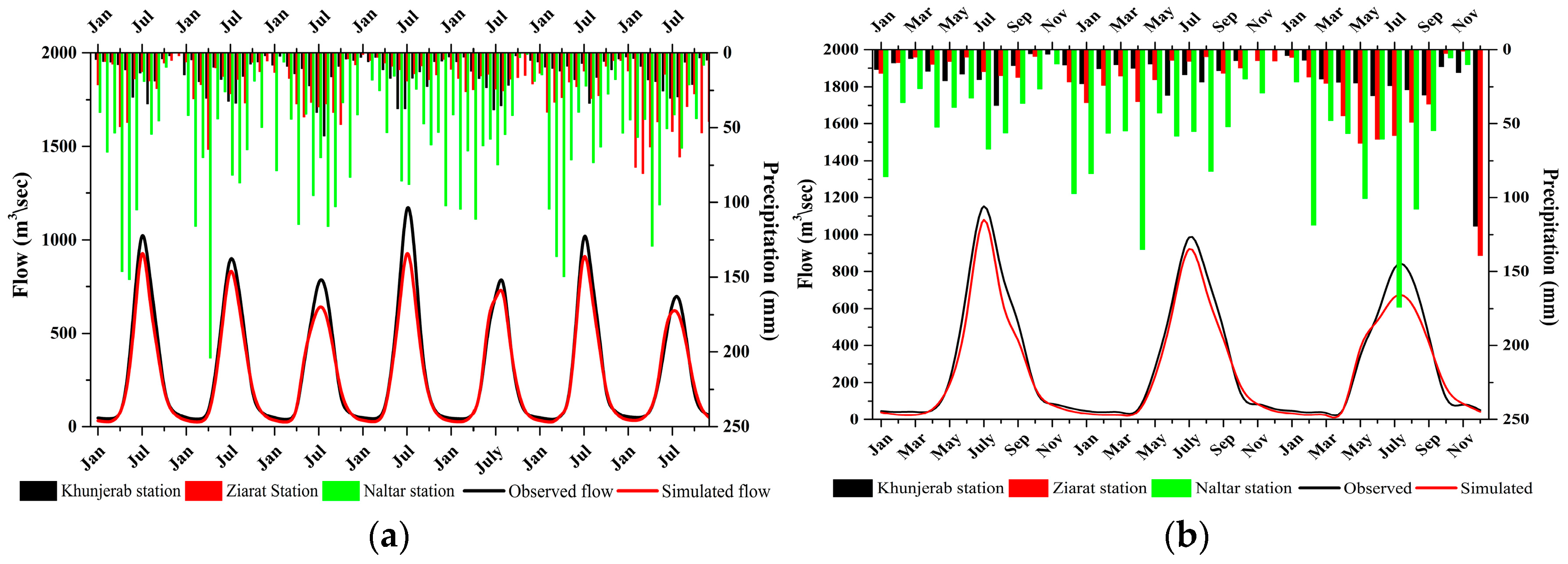
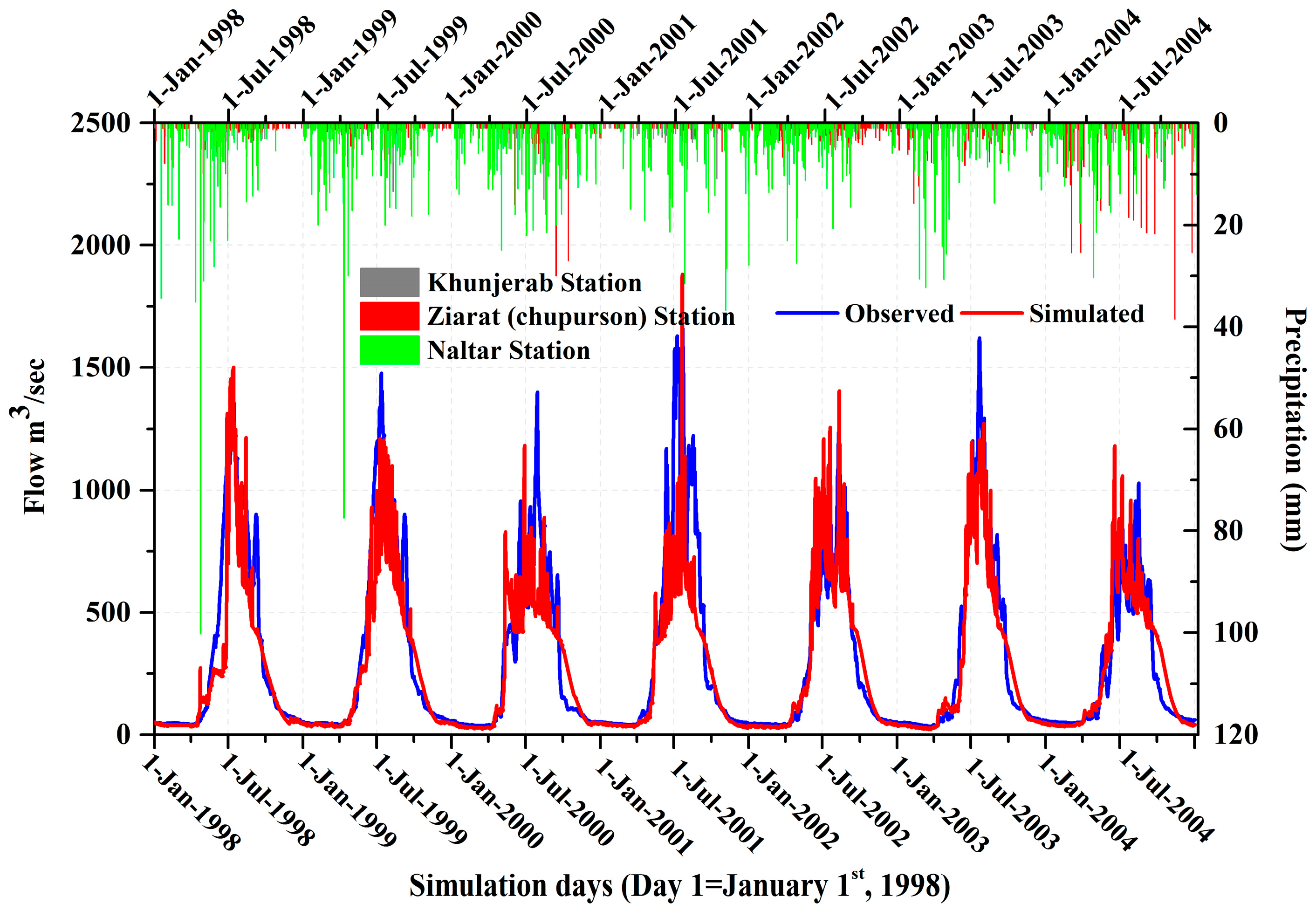
The performance indicators for the model parameters were derived using daily-based datasets (Table 4). The calibration results revealed observed flow peaks for the year 2001 and lowest flows for 2004 (Figure 4). From the visual analysis of simulated and observed hydrographs, the timing of the peak is regenerated well while the simulation high flow peaks showed underestimation, especially during the dry-years (e.g., 1999, 2000, and 2003) probably due to the present curve number (CN) technique, which is unable to generate accurate runoff prediction for a day that are influenced by different storm and wind situations. When storms occur during a single day, the level of soil moisture and the corresponding runoff CN vary from storm to storm [41]. However, the SCS-CN approach defines a rainfall event as the sum of all rainfall that occurs during one day, and this might lead to underestimation of peak runoff [42]. Similarly, other factors (topographic properties, aspects, slope, soil, and different land use/cover) also have an effect on the peak flow, snow accumulation and melt processes [12]. The p-factor and r-factor values were 0.45 and 0.25 during the calibration period (1998–2004) and these were 0.79 (p-factor) and 0.85 (r-factor) for the validation period (2008–2010), respectively (Table 4). During the calibration period, the observed data in percent by 95PPU was 97% whereas during validation period it was 85%, which indicated that the model results were good in terms of percentage of the data being bracketed (p-factor), but the uncertainty was larger as shown by the r-factor. In the Hunza watershed, the model showed large uncertainties for extreme events during both the calibration and validation periods. The study area was highly snow and glacier covered and mountainous, where snowfall was a very important factor (>60% of total precipitation). The SWAT classified precipitation as snow or rainfall using the average daily temperature data. The model simulated discharge from highly snow and glacier covered watersheds was well calibrated by the SWAT model. Similar results were observed by [43,44]. Rahman et al. [37] found that modified routines improved the model’s annual stream flow prediction with an R² value of >0.8 compared to an initial R² value of <−0.7. The parameters’ uncertainties were satisfactory, when the parameter ranges of the p-factor and r-factor reached the initial required limits. 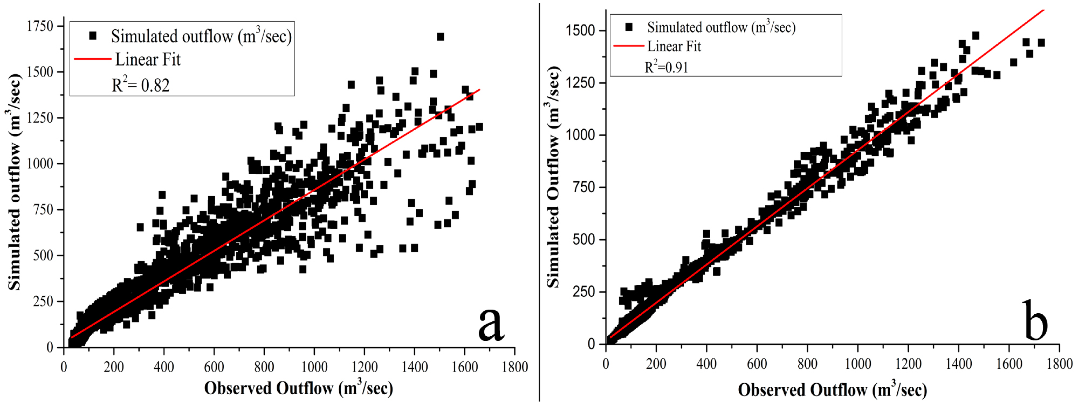During the calibration period, the values of R² and NS generated by the model were 0.82 and 0.80 respectively, while for the validation period (R² and NS) obtained values were 0.91 and 0.87, respectively (Table 4), which indicated that the model could be acceptable for the Hunza watershed.

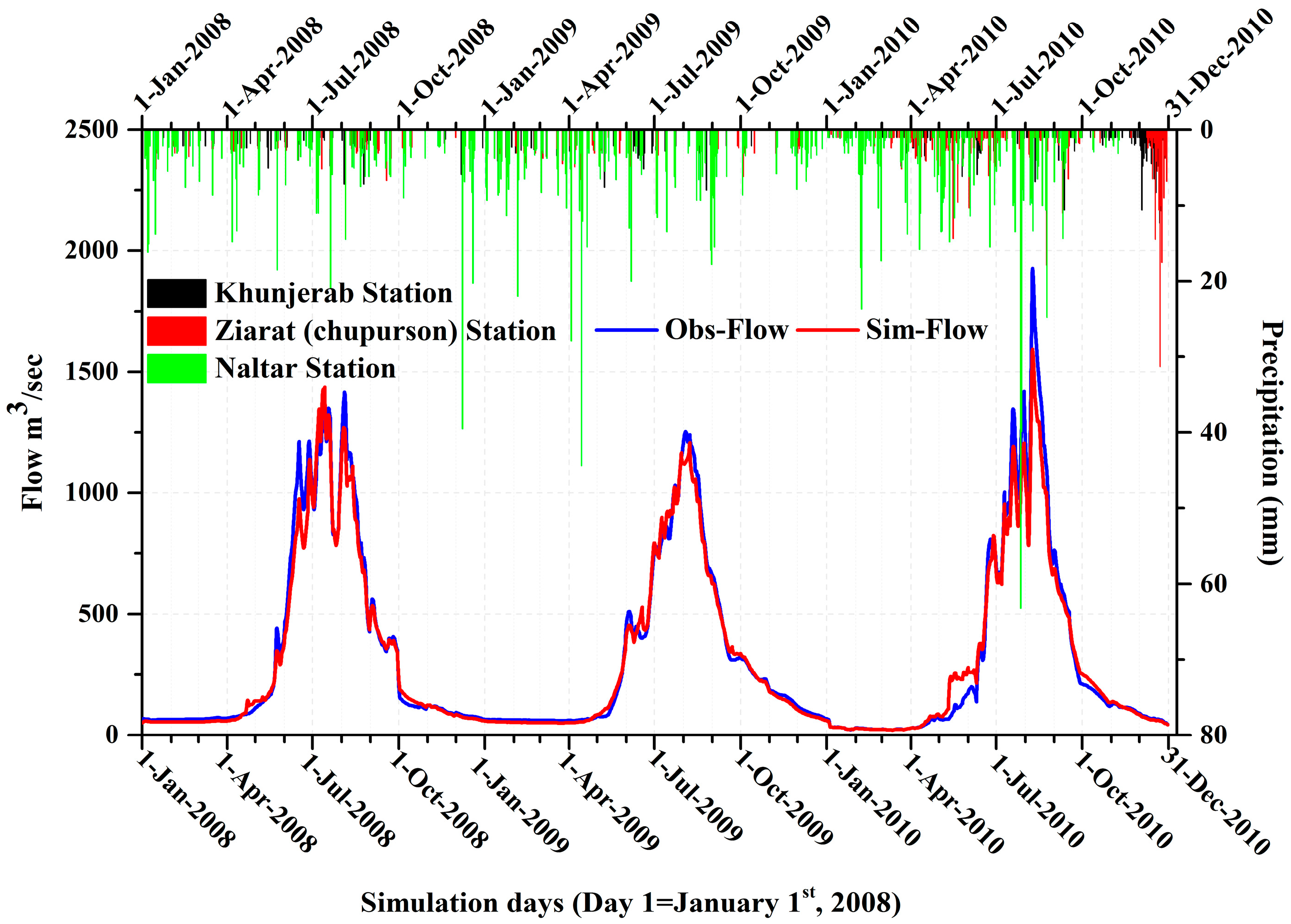
The statistical results for the calibration (1998–2004) and validation (2008–2010) periods of the Hunza River flows (Table 4, Figure 5a,b) indicate that the model produced satisfactory results for both the periods.

Daily stream flows were steadily underestimated by SWAT; these trends might be explained in terms of the temperature index with elevation bands approach, which is used for modelling snow and glacier melt in SWAT. Many different parameters affect snow extent and melting processes, including altitude, topography and terrain, aspect, slope and land-cover/use. However, such parameters are not well represented in the temperature index with elevation bands method [12]. This could possibly be a reason for not showing the insignificant impact of the catastrophic incidence of Attaabad Lake (initially, 24 km long and 130.032 m deep with surface area of 10,414 km²) was formed on Hunza River due a massive landslide that occurred on 4 January 2010, took 20 precious human lives and rendered another 392 families homeless, and blocked Hunza River for about five months (4 January–27 May 2010) [45] formation on downstream flow in Hunza.

The river was at its peak during winter (January–May 2010) when snow and glacier-melt contribution from the high-altitude catchments of the Hunza River sub basin was negligible, except the base flow (Figure 4). Ground water parameters also affect the timing of ground water supply to the stream flow. Low values of the base flow (ALPHA_BF) reduce the model efficiency to induce snow-melt recharge, which can increase the amount of runoff in the future (later in the year).

However, lower values of ALPHA_BF also decreased the snow and glacier melt runoff by decreasing the contribution of ground-water and increased the stream flow during the off season of the snow-melt period, when the stream flow was quickly shifting from a dominant regime of shallow sub-surface flow to one of the groundwater flows. Decreasing the GW_DELAY value moderately balanced the effect of limited base flow on the stream flow peak, but the model performance results improved during the base flow period, and on larger scale displayed reduced model performance during the runoff period (

Table 5. Simulated daily average water balance components and their values.

Component of Water Balance (mm)	Calibration (1998–2004)	Validation (2008–2010)
Yearly precipitation	388.6	325.4
Potential evapotranspiration (PET)	77.6	67.10
Actual evapotranspiration (AET)	43.7	44.5
Water yield (WYLD)	57.39	53.40
Surface runoff (Sur_Q)	176.92	145.83
Soil water (SW)	34.71	30.20
Lateral flow (Lat_Q)	125.87	122.67
Contribution of groundwater to stream flow (Gw_Q)	31.44	27.54

).

According to daily stream flow results, PBIAS values of 3.9 and 1.8 for the calibration and validation periods were recorded which showed that the model overestimated the stream flow during the validation period and produced a less accurate model simulation for the calibration period. The results showed RSR values of 0.45 for the calibration period and 0.59 for the validation period. The statistical evaluation of the simulated and observed daily stream flow data is summarized in Table 4. After applying the model evaluation recommended by the statistical techniques mentioned above, it was found that the model was quite efficient and that the results were reliable.

The model results for monthly flow are presented in Figure 6a,b, where they appeared to be quite reasonable. The simulation predicts that the peak flow values occurred in the months of January, May and September. The peak positions were generally well distributed and representative for both the calibration and validation periods. It is clear that given more reliable precipitation and temperature datasets from the meteorological observatories with good spatial coverage of the study area, more accurate results could have been obtained from the model. Low stream flow is predicted during the top events by the SWAT model, which was reported in many previous studies [46]. The descriptive statistics of the average monthly flows are summarized in

Table 6. Simulated daily average water balance components and their values.

Average Monthly Values (mm) for the Hunza River Basin
Month	Precipitation (mm)	Snow Fall (mm)	Surf Q (mm)	Lat Q (mm)	Water Yield (mm)	ET (mm)	PET (mm)
1	19.03	18.66	0.55	0.6	1.8	0.01	0.02
2	33.21	26.66	12.75	6.75	20.02	0.02	0.02
3	32.6	15.07	34.02	21.25	57.39	0.7	0.97
4	61.46	7.19	32.45	17.16	54.27	3.4	5.39
5	34.32	3.89	27.19	11.24	43.68	5.45	10.07
6	38.04	2.82	18.08	12.51	34.4	8.06	14.06
7	39.11	0.75	13.83	15.92	32.63	8.81	16.97
8	45.2	0.84	16.09	18.19	37.65	8.45	14.93
9	32.74	2.48	11.29	11.52	26.32	5.66	9.75
10	20.24	4.63	5.88	6.19	15.01	2.36	4.17
11	15.35	6.44	4.39	3.74	10.18	0.67	1.08
12	18.07	16.34	0.71	0.98	3.09	0.11	0.17

.

We analysed, quantified and handled different types of water management issues and hydrological processes induced by changes in temperature and precipitation in the study area. The SWAT model calculated the remaining water balance components of daily and monthly flows in Table 5. Studies [47] noted that surface runoff, precipitation/snow fall, lateral flow, base flow and evapotranspiration are important elements of the water balance. For each of these variables, prediction is not easy, except in the case of precipitation. The daily average values of different water balance variables in the basin during the calibration and validation periods, as calculated by the SWAT model, are given in Table 4 with their relative percentages to daily average rainfall. Of these variables, ET contributed the largest volume of water loss from the catchment area during flow. High evapotranspiration rates and relatively moderate temperatures implied the presence of heterogeneous vegetation cover types in the study area. The monthly average values of precipitation, ET, water yield (WYLD), snow fall, soil yield, lateral flow (Lat Q) and evaporation are given in Table 5.

We calculated the daily flow contribution to the Indus River for the purposes of future water management in the area. The estimated daily river flow from the Hunza River as per the SWAT model was based on the downstream runoff to the entire outlet of the watershed at Danyore. The simulated values were compared with recorded daily inflow values (Figure 5a,b) for the calibration and validation periods. Results obtained showed a strong correlation between the calibration and validation periods. Therefore, the calibrated model can be used to predict the volume inflow to the Indus River system, to inform stakeholders about future water storage and sustainable management of existing and upcoming water reservoirs, such as the Diamer-Basha Dam, downstream of the Indus River in Pakistan.

4.1. Future Climate Projections (2010–2100)

The SSRC is validated by verifying the agreement of the fractional wetted day’s area of simulation (FWA_S) with gauged average daily values of the fractional wetted days area (FWA_G) for each rain gauge station data has been taken by individual and combine. Similarly, second-order statistics also performed for daily single station observed precipitation (RG_i) and simulated yearly accumulated precipitation (RGcumi) are represented in

Table 7. Back-casting station wise comparison of second-order moments of daily precipitation (Mean and Standard Deviation) of all stations for 30 years of data.

Stations	Mean RG	St. Dev RG	Mean RSi	St. Dev RSi
Khunjerab	3.66	11.33	3.38	19.84
Ziarat	3.96	10.23	3.38	18.59
Naltar	3.96	10.76	3.38	22.55
Gilgit	4.13	10.55	3.24	17.14
Gupis	3.74	8.85	3.20	15.89
Skardu	3.22	10.76	3.47	13.49

. Generally, the model performs well in preserving the spatial irregularity of the data, and the average yearly simulated wetted area at the suitable scale of (FWAs = 0.49) with (FWA_G = 0.52 and p-value = 0.63). All the observed results are acceptable and suitable for data downscaling.

We also validate the downscaling of GCM with the control period from 1980 to 2010 with a different precipitation gauge station of the study area. Firstly, we corrected and validated Bias_GAO by comparing a sample fraction of wet days in the simulated series R_SA, p_os against its R_GA series. In the next step of data processing, we compared second-order statistics of the daily-based calculated rainfall area (R_SA = R_GCM.Bias_GAO) with those of the random gauge average (R_GA). The wet day’s fraction (p_o) is well defined and the yearly simulated average value is 37.2% against the wet day’s fraction (37.3%) with p-value (0.47), and similarly good results indicate seasonal values. From the results, it is clear that the model also suitably depicts daily wet–dry spells arrangement. After that, we investigate the relationship between daily average simulated precipitation (R_SA) = 3.45 mm⁻¹ with standard deviation (6.89 mm⁻¹) and the average daily observed station values R_GA = 3.47 mm⁻¹ with standard deviation (6.56 mm⁻¹). A good relationship agreement is found with p-values (0.59 and 0.04) for mean and standard deviation respectively, and a similar good fitting result is also observed (mean values) for each season, and the same type of results are also observed by [33] for Italy.

High-resolution future climate projections acquired by CCSM4, EC-EARTH and ECHAM6 downscaled under the three Representative Concentration Pathways scenarios (RCP2.6, RCP4.5 and RCP8.5) were used to calculate future climate (temperature and precipitation). Monthly climate change for the two periods (2030–2059 and 2070–2099) against the control period (1980–2010) for temperature and precipitation is summarized in

Table 8. Monthly temperature variation (°C) against control period for our future reference years.

2030–2059	GCMs	January	February	March	April	May	June	July	August	September	October	November	December	Annually
RCP2.6	EC-EARTH	1.32	1.02	0.5	1.4	1.32	1.3	1.46	1.39	0.82	1.27	2.59	2.3	1.39
	CCSM4	1.39	0.25	−0.33	−0.22	0.45	0.79	1.49	1.73	21.76	2.89	2.75	2.19	2.93
	ECHAM6	1.52	0.61	1.59	1.31	0.74	1.28	2.36	1.14	1.56	1.52	2.39	1.31	1.44
RCP4.5	EC-EARTH	1.32	1.02	0.5	1.4	1.32	21.3	1.46	1.39	0.82	1.27	2.59	2.3	3.06
	CCSM4	1.39	0.25	−0.13	−0.22	0.45	0.79	1.49	1.73	2.76	2.89	2.75	2.19	1.36
	ECHAM6	1.52	0.61	1.59	1.31	0.74	1.28	2.36	1.14	1.56	1.52	2.39	1.31	1.44
RCP8.5	EC-EARTH	1.52	1.65	1.75	2.28	1.89	1.73	0.97	0.89	2.4	2.46	2.04	1.57	1.76
	CCSM4	2.35	1.31	0.76	0.98	2.66	1.89	2.09	2.35	2.83	3.65	3.89	2.34	2.26
	ECHAM6	1.05	0.97	1.28	1.53	1.14	1.33	2.28	1.85	3.2	2.57	2.09	1.45	1.73
2070–2099	GCMs	January	February	March	April	May	June	July	August	September	October	November	December	Annually
RCP2.6	EC-EARTH	1.54	0.67	1.04	−0.46	1.98	0.75	0.65	1.13	0.67	0.88	−0.3	2.09	0.89
	CCSM4	0.45	0.63	0.3	0.32	−0.18	−0.51	0.74	1.27	2.63	2.2	2.09	0.95	0.91
	ECHAM6	−0.45	0.75	1.36	1.23	0.76	0.37	1.24	0.89	0.66	1.76	0.72	0.18	0.79
RCP4.5	EC-EARTH	3.75	3.16	2.44	2.78	3.01	2.67	3.24	3.54	3.45	3.59	2.67	2.09	3.03
	CCSM4	2.65	2.24	1.03	0.83	1.1	1.05	2.65	2.52	3.84	3.64	2.09	2.35	2.17
	ECHAM6	3.5	1.97	3.05	2.07	1.45	2.34	3.23	2.38	3.26	2.55	2.76	2.96	2.63
RCP8.5	EC-EARTH	4.06	3.96	5.78	5.97	5.44	4.65	5.02	5.74	5.67	6.66	6.25	5.57	5.40
	CCSM4	4.78	4.39	4.06	4.16	4.91	3.29	5.47	6.02	6.61	9.98	6.43	5.81	5.49
	ECHAM6	5.76	4.83	5.29	5.09	4.65	6.08	6.76	5.46	5.33	6.45	6.46	6.34	5.71

and

Table 9. Monthly precipitation variation (%) against the control period for our future reference years.

2030–2059	GCMs	January	February	March	April	May	June	July	August	September	October	November	December	Annually
RCP2.6	EC-EARTH	13.75	10.65	23.7	−10.9	10.67	24.04	6.59	16.69	25.89	−15.43	5.88	−19.5	7.67
	CCSM4	−26.9	15.03	−32.9	24.95	−5.83	−8.43	2.54	38.14	−21.07	−67.3	75.37	−14.0	−1.70
	ECHAM6	13.0	−34.5	25.8	−12.8	38.8	0.4	−6.2	25.0	18.0	−48.4	−23.2	22.0	1.49
RCP4.5	EC-EARTH	10.8	46.5	4.9	43.2	−13	−7.4	16.5	3.1	−2.2	50.5	−27.6	−4.4	10.08
	CCSM4	66.9	10.54	−7.7	25.3	−20.43	38.9	−10.99	−43.8	−27.2	−49.5	−49.6	−22.2	−7.48
	ECHAM6	10.56	20	−15.3	3.87	35.5	−41.6	−20.7	18	12.2	−12.4	−6.2	35.4	3.28
RCP8.5	EC-EARTH	19.0	9.2	−16.4	49.03	7.6	12.7	77.2	20.2	11.3	34.5	−40.8	44.2	18.98
	CCSM4	4.97	14.8	−25.5	5.5	−3.18	49.3	−19.34	−20.93	−23.3	−29.56	−34.54	0.1	−6.81
	ECHAM6	−17.6	−13.4	−16.9	−17.0	23	−29.3	−8.5	13.6	−9.7	20.13	−27.4	29	−4.51
2070–2099	GCMs	January	February	March	April	May	June	July	August	September	October	November	December	Annually
RCP2.6	EC-EARTH	12.0	22.43	−8.9	21.0	−45.5	47.3	−2.7	11.5	1.03	22	−31.8	−14.2	2.85
	CCSM4	38.43	2.67	−18.7	57.6	12.1	−20.23	2.3	2.7	−12.45	30.76	−34.5	15.4	6.34
	ECHAM6	11.01	−24.1	18.6	−14.6	12.0	−18.4	7.65	6.33	3.3	107	−7.4	67.55	14.08
RCP4.5	EC-EARTH	−23.3	32.1	−18.0	13.6	17.4	39.65	23.02	−10.8	−17.0	35.2	−34.7	86.4	11.96
	CCSM4	10.1	16.6	24.4	24.2	21.9	24	25.4	27.7	21.3	17.9	16.5	12.1	20.18
	ECHAM6	−32.5	−0.5	23.45	25.43	57.1	−11.4	2.04	9.56	−7.7	−6.7	−0.4	5.2	5.30
RCP8.5	EC-EARTH	52.8	23.7	72.0	42.0	8.0	38.9	37.1	−27.9	−11.5	43	−1.4	95.2	30.99
	CCSM4	21.8	−39.7	−19	27.0	55.8	102.8	−30.9	17.4	−6.2	−6.1	−27.3	8.5	8.68
	ECHAM6	23.55	−34.3	−3.5	−17.3	27.4	−1.99	−13.6	−1.45	65.5	56.4	−85.7	22.8	3.15

. Temperature was of serious concern, as all the model scenarios indicated an increasing trend of 0.89, 3.03 and 5.40 °C towards the end of this century (2100) under the respective RCPs scenarios, except in a few cases where monthly predicted future temperature simulation increased towards midcentury as compared to the referenced data period (1980–2010), ranging between 1.39 (EC-EARTH under RCP2.6) and 2.26 °C (CCSM4 under RCP8.5) shown in Table 8. Under the scenario RCP2.6 long-term projection, temperature was lower at the end of century as compared to the midcentury, but still temperature values were higher than the current value (lower temperature increase was 0.79 °C as indicated by the ECHMA6 at the end of this century, with reference to the control period (1980–2010) and −0.65 for respective RCP2.6 (2030–2059) variation) whereas, the end of the century temperature increase was in the range of 2.17 °C to 3.03 °C (RCP4.5) and 5.40 °C to 5.71 °C (RCP8.5) with reference to current temperature value.

Kazmi et al. [48] and Islam et al. [49] projected a future temperature increase in the UIB region under different scenarios (A2 and A1B) using PRECIS RCM data, while [11]., also using PRECIS RCM data, projected an increase in annual mean temperature of 4.88 °C by the end of this century in the upper Indus Basin. Rajbhandari et al. [50] also found the same results of increasing projected temperatures in the Indus Basin using PRECIS RCM data. The above cited studies suggest that there has been an overall projected temperature gradual increase in the UIB, but with little difference in the defined seasonal trends.

Generally, projected precipitation had increased, but results of the model scenarios were totally different. The first RCP4.5 (2030–2059) with the CCSM4 model showed a minor annual decreasing trend but towards the end of this century, the precipitation trend was increasing with a 31% variation in all scenarios.

Midcentury (2030–2059) annual precipitation change as compare to Naltar (125 mm·year⁻¹ during 1980–2010) annual precipitation change is varied from 1.49% to 7.67% with ECHAM6 and EC-EARTH models, respectively under the RCP2.6 scenario, and 3.28% to 19.58% under the RCP4.5 scenario with CCSM4 and ECHAM6 models respectively, and from −7.48% to 10.08% under the scenario of RCP8.5 with ECHAM6 and EC-EARTH models respectively (Table 9), showing a variation range liable on the model inputs, scenario and season. During the projected period (2070–2099), projected precipitation had continuously increased by 14.08%, 20.18% and 30.99% for the RCP2.6, RCP4.5 and RCP8.5 with the climate models ECHAM6, CCSM4 and EC-EARTH respectively.

The projected precipitation increase in the UIB region is reported by [15] to be 25% compared to baseline by 2046–2065 based on five GCMs (for A1B International Journal of Water Resources Development 205 scenarios), while [17] projected an increase of up to 21% using the PRECIS high-resolution regional climate model (RCM). Rajbhandari et al. [50] also projected an increase in precipitation over the UIB for the A1B scenario by the end of this century. Similarly, Forsythe et al. [51] also projected an increase in precipitation in the upper Indus Basin (maximum seasonal mean 27%, annual mean change 18%) using a stochastic rainfall model, with increased intensity in the wettest months (February, March and April).

The values of future climate projections primarily depend on the GCMs used as a driver. All the cited above studies predict an overall increase in precipitation, while details and methodology used differ.

4.2. Future Hydrological Flows (2010–2100)

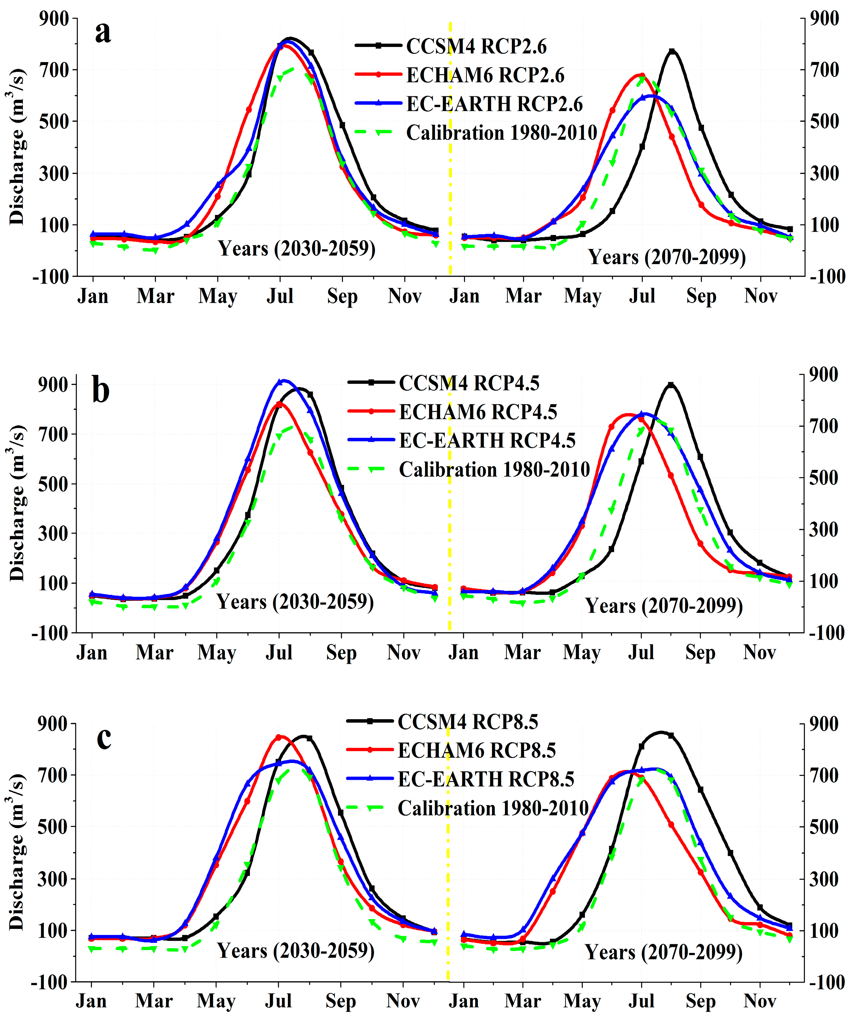
Monthly discharge under different climatic scenarios with decadal reference data (Figure 7) showed a positive projection for future annual discharge variations during the period 2030–2059, with an increase flow of 23.77%–28.57%, 27.81%–43.70% and 10.63%–22.27% for RCP2.6, RCP4.5 and RCP8.5, respectively. According to ECHAM6, mean annual discharge E(Q) increased by 1154 mm·year⁻¹ as compared to CP under the scenario RCP2.6; 1277 mm·year⁻¹ under RCP4.5 (EC-EARTH); and 1156 mm·year⁻¹ under RCP8.5 (ECHAM6). The discharge situation was almost similar towards the end of this century for the scenarios RCP2.6 and RCP8.5, but RCP4.5 indicated a slight increase (15.83%–32.12%). RCP2.6 showed 7.57%–31.12% for all models. Under the climatic scenario RCP2.6, E(Q) indicated a decreasing trend of 11.56% (913 mm·year⁻¹), and E(Q) increased under climatic scenario RCP4.5 reaching 1107 mm·year⁻¹ and 1283 mm·year⁻¹ for scenario RCP8.5, which was less than the mid-century mean annual flow, but still higher than the Control Period (CP).

A few statistical indicators i.e., Q37, Q91, Q182, and Q274 were also estimated but not displayed under different climatic scenarios averaged on the reference decades, to compare individually in the CP. Yearly decadal average values of the highest and lowest flows anticipated in the Hunza river basin for gradually longer periods d, Q_M,d, and Q_m,d, for values of d = 37, 91, 182, and 274 days were also computed.

Selected river flow lemmas in exercise remained higher than in the CP situation during the 2030–2059 period, and showed decreasing values by EC-EARTH under all states during 2070–2099. Results for the future climatic projections showed that the projected hydrological cycle displayed different conditions for midcentury, depending upon which GCM model was accepted to feed the hydrological model. The EC-EARTH hydrological model showed a decreasing trend in winter and a substantially increasing trend during spring. Similarly, ECHAM6 exhibited a minor decreasing trend during August–December (−5% to −23%) and an increasing trend in the remaining months, especially in spring (February–April). The CCSM4 model provided totally reverse results for discharge, with a −25% decrease during spring but a slightly increasing trend for all other months.

In the second future reference years, the overall discharge shape remained the same for autumn and winter. In spring hydrological projection models (ECHAM6 and EC-EARTH) are provided the highest increase in discharge due to early melting of snow. These are resulted from the increasing of temperature which is followed by winter precipitation (snowfall) with a discharge volume of 100% in April ECHAM6 and EC-EARTH under the RCP8.5 scenario. The discharge was still high in the spring at the end of this century (2100). On the contrary, in July and August, flow discharge volumes decreased. In the RCP2.6 scenario, river discharge was less than in the CP, which was perhaps because of the decreasing lower elevation ice mass coupled with the increasing temperature yield. The precipitation regimes had a high impact on discharge variability in the region.

Similar results were found by [11], who analyzed the projected impact of climate change in the Hunza, Gilgit and Astore sub-basins using the PRECIS regional climate model with the SRES A2 scenario. Similarly [15,52,53] studied the impact of climate change on the upstream area of the Indus Basin under the different climatic scenarios in different numbers of GCMs which represent variations in future climate ranging from dry and cold to wet and warm. Most of the climate-model data suggested that annual runoff will increase by 7.57%–32.12% towards the end of century (2100), resulting in an increase in temperature (1.39 °C to 6.58 °C) and precipitation (31%). However, the projected future hydrology depends on the accelerated melt and projected precipitation in the UIB, which have a large uncertainty and large variation between average seasonal and annual projections among the GCMs. From the above given results, it is clear that the greatest source of uncertainty regarding the future climate change on streamflow is dependent on the structure of GCM (means choice of GCM). Moreover, the concept of the hydrological models brings another level of uncertainty.

5. Conclusions

The potential impact of climate change on stream flow in the Hunza River, downstream of the Hunza River sub-basin watershed, was analyzed using three GCMs by the IPCC fifth report on climate scenarios with the SWAT hydrological model. The SWAT model was successfully applied on hydrological date from the Hunza river basin at the Danyore gauge station while using an advance SUFI-2 calibration, validation, sensitivity and uncertainty analysis algorithm.

From the results and evaluation criteria, the SWAT model performed best for both the calibration and validation periods. Results showed a high degree of efficiency of the model for the snowy and glaciated sub-basins of the Hunza River.

The proposed downscaling methodology for precipitation from a GCM under a control period can be well represented using a random cascade statistical approach. The method given by BIAS_GAO plus SSRC seems capable of being repeated realistically well for the single station precipitation gauge data of the catchment. Future climate variability in terms of temperature and precipitation showed that the climate in the study area will become warmer and wetter under the majority of the scenarios predicted, except for CCSM4 with RCP4.5 scenarios, where a slightly decreasing annual precipitation trend was predicted towards the middle of this century, followed by a 31% increase in all scenarios by end of the century. Like precipitation, temperature will also increase towards the end of this century by 1.39 °C to 5.71 °C (with different climatic scenarios and models) with respect to present day temperature values. The above future climatic change conditions are converted into a possible range of stream flows using the SWAT model. This model indicates that flow change towards 2060 will predict to be increased by 10.63%–43.70% for different RCPs. The similar situation is also expected at the end of this century for the scenario RCP8.5, nevertheless RCP4.5 indicates a slight increase (9.38%–32.12%) and only RCP2.6 shows a decrease (11.56%) for all future climate models. Seasonally, stream flow changes are predicted to be in range of 19%–27% for all seasons, based on the results of this simulation.

In the light of above results and discussion, we have concluded here that the Hunza watershed runoff volume will experience a slight decrease at the end of the century as compared to mid-century, nevertheless, it is higher than current flow. Although the future flow projections shown here may not be accurate due to uncertainties in climate change scenarios and GCMs outputs, they are still suitable for calibration and validation in the snowy and glaciated areas. The results of this analysis should therefore be considered for and incorporated into water resources management plans for future water storage in the Diamer-Basha Dam and other upcoming reservoirs in the Indus River system. This model can also be used for future land-use and land-cover impact assessments on water resources. It is also suggested to use more uncertainty techniques in model calibration, validation, sensitivity and uncertainty analyses.

References

1. Immerzeel, W. Spatial Modeling of Mountainous Basins: An Integrated Analysis of the Hydrological Cycle, Climate Change and Agriculture; Netherlands Geographical Studies; Utrecht University: Utrecht, The Netherlands, 2008; Volume 369. [Google Scholar]
2. Tahir, A.; Chevallier, P.; Arnaud, Y.; Ahmad, B. Snow cover dynamics and hydrological regime of the Hunza river basin, Karakoram range, Northern Pakistan. Hydrol. Earth Syst. Sci. 2011, 15, 2259–2274. [Google Scholar] [CrossRef] [Green Version]
3. Debele, B.; Srinivasan, R.; Gosain, A. Comparison of process-based and temperature-index snowmelt modeling in SWAT. Water Resour. Manag. 2010, 24, 1065–1088. [Google Scholar] [CrossRef]
4. Young, G.; Hewitt, K. Hydrology research in the Upper Indus Basin, Karakoram Himalaya, Pakistan. Hydrol. Mt. Areas. IAHS Publ. 1990, 190, 139–152. [Google Scholar]
5. Hewitt, K.; Wake, C.; Young, G.; David, C. Hydrological investigations at Biafo glacier, Karakorum Range, Himalaya; an important source of water for the Indus river. Ann. Glaciol. 1989, 13, 103–108. [Google Scholar]
6. Bookhagen, B.; Burbank, D.W. Toward a complete Himalayan hydrological budget: Spatiotemporal distribution of snowmelt and rainfall and their impact on river discharge. J. Geophys. Res. Earth Surf. 2010, 115, F03019. [Google Scholar] [CrossRef]
7. United Nations Development Programme (UNDP). Community Based Survey for Assessment of Glacier Lake Outburst Flood Hazards (GLOFs) in Hunza River Basin; UNDP Report; UNDP: Islamabad, Pakistan, 2008. [Google Scholar]
8. Zhang, X.; Srinivasan, R.; Hao, F. Predicting hydrologic response to climate change in the Luohe river basin using the SWAT model. Trans. ASABE 2007, 50, 901–910. [Google Scholar] [CrossRef]
9. Singh, A.; Gosain, A. Climate-change impact assessment using GIS-based hydrological modelling. Water Int. 2011, 36, 386–397. [Google Scholar] [CrossRef]
10. Sood, A.; Muthuwatta, L.; McCartney, M. A SWAT evaluation of the effect of climate change on the hydrology of the Volta river basin. Water Int. 2013, 38, 297–311. [Google Scholar] [CrossRef]
11. Akhtar, M.; Ahmad, N.; Booij, M. The impact of climate change on the water resources of Hindukush–Karakorum–Himalaya region under different glacier coverage scenarios. J. Hydrol. 2008, 355, 148–163. [Google Scholar] [CrossRef]
12. Pradhanang, S.M.; Anandhi, A.; Mukundan, R.; Zion, M.S.; Pierson, D.C.; Schneiderman, E.M.; Matonse, A.; Frei, A. Application of SWAT model to assess snowpack development and streamflow in the Cannonsville watershed, New York, USA. Hydrol. Process. 2011, 25, 3268–3277. [Google Scholar] [CrossRef]
13. Khan, A.; Ghoraba, S.; Arnold, J.G.; Di Luzio, M. Hydrological modeling of upper Indus basin and assessment of deltaic ecology. Int. J. Mod. Eng. Res. (IJMER) 2014, 4, 73–85. [Google Scholar]
14. Shrestha, M.; Koike, T.; Hirabayashi, Y.; Xue, Y.; Wang, L.; Rasul, G.; Ahmad, B. Integrated simulation of snow and glacier melt in water and energy balance-based, distributed hydrological modeling framework at Hunza river basin of Pakistan Karakoram region. J. Geophys. Res. Atmos. 2015, 120, 4889–4919. [Google Scholar] [CrossRef]
15. Immerzeel, W.W.; Van Beek, L.P.; Bierkens, M.F. Climate change will affect the Asian water towers. Science 2010, 328, 1382–1385. [Google Scholar] [CrossRef] [PubMed]
16. Konz, M.; Uhlenbrook, S.; Braun, L.; Shrestha, A.; Demuth, S. Implementation of a process-based catchment model in a poorly gauged, highly glacierized Himalayan headwater. Hydrol. Earth Syst. Sci. Discuss. 2007, 11, 1323–1339. [Google Scholar] [CrossRef] [Green Version]
17. Akhtar, M.; Ahmad, N.; Booij, M. Use of regional climate model simulations as input for hydrological models for the Hindukush-Karakorum-Himalaya region. Hydrol. Earth Syst. Sci. 2009, 13, 1075–1089. [Google Scholar] [CrossRef]
18. Neitsch, S.L.; Arnold, J.G.; Kiniry, J.R.; Williams, J.R. Soil and Water Assessment Tool Theoretical Documentation Version 2009; Texas Water Resources Institute: College Station, TX, USA, 2011. [Google Scholar]
19. Wake, C.P. Glaciochemical investigations as a tool for determining the spatial and seasonal variation of snow accumulation in the central Karakoram, Northern Pakistan. Ann. Glaciol. 1989, 13, 279–284. [Google Scholar]
20. Tachikawa, T.; Kaku, M.; Iwasaki, A.; Gesch, D.; Oimoen, M.; Zhang, Z.; Danielson, J.; Krieger, T.; Curtis, B.; Haase, J. ASTER Global Digital Elevation Model Version 2—Summary of Validation Results; NASA: Washington, DC, USA, 2011.
21. Nachtergaele, F.; van Velthuizen, H.; Verelst, L.; Batjes, N.; Dijkshoorn, K.; van Engelen, V.; Fischer, G.; Jones, A.; Montanarella, L.; Petri, M. Harmonized World Soil Database; Food and Agriculture Organization of the United Nations: Rome, Italy, 2008. [Google Scholar]
22. Arnold, J.G.; Srinivasan, R.; Muttiah, R.S.; Williams, J.R. Large area hydrologic modeling and assessment part I: Model development 1. Jawra J. Am. Water Resour. Assoc. 1998, 34, 73–89. [Google Scholar] [CrossRef]
23. Abbaspour, K.; Vejdani, M.; Haghighat, S. SWAT-CUP calibration and uncertainty programs for SWAT. In Proceedings of the MODSIM 2007 International Congress on Modelling and Simulation, Christchurch, New Zealand, 10–13 December 2007; Oxley, L., Kulasiri, D., Eds.; Modelling and Simulation Society of Australia and New Zealand: Christchurch, New Zealand, 2007; pp. 74–80. [Google Scholar]
24. Winchell, M.; Srinivasan, R.; Di Luzio, M.; Arnold, J. Arc SWAT Interface for SWAT2005 User’s Guide; Texas Agricultural Experiment Station and United States Department of Agriculture: Temple, TX, USA, 2007.
25. Gitau, M.W.; Chaubey, I. Regionalization of SWAT model parameters for use in ungauged watersheds. Water 2010, 2, 849–871. [Google Scholar] [CrossRef]
26. Abbaspour, K.C. SWAT-CUP4: SWAT Calibration and Uncertainty Programs—A User Manual; Swiss Federal Institute of Aquatic Science and Technology, Eawag: Dübendorf, Switzerland, 2011. [Google Scholar]
27. Abbaspour, K.C.; Faramarzi, M.; Ghasemi, S.S.; Yang, H. Assessing the impact of climate change on water resources in Iran. Water Resour. Res. 2009, 45. [Google Scholar] [CrossRef]
28. Nash, J.E.; Sutcliffe, J.V. River flow forecasting through conceptual models part I—A discussion of principles. J. Hydrol. 1970, 10, 282–290. [Google Scholar] [CrossRef]
29. Krause, P.; Boyle, D.; Bäse, F. Comparison of different efficiency criteria for hydrological model assessment. Adv. Geosci. 2005, 5, 89–97. [Google Scholar] [CrossRef]
30. Soncini, A.; Bocchiola, D.; Confortola, G.; Bianchi, A.; Rosso, R.; Mayer, C.; Lambrecht, A.; Palazzi, E.; Smiraglia, C.; Diolaiuti, G. Future hydrological regimes in the Upper Indus basin: A case study from a high-altitude glacierized catchment. J. Hydrometeorol. 2015, 16, 306–326. [Google Scholar] [CrossRef]
31. Qin, D.; Plattner, G.; Tignor, M.; Allen, S.; Boschung, J.; Nauels, A.; Xia, Y.; Bex, V.; Midgley, P. Summary for Policymakers. Climate Change 2013: The Physical Science Basis. Contribution of Working Group I to the Fifth Assessment Report of the Intergovernmental Panel on Climate Change; Cambridge University Press: Cambridge, UK; New York, NY, USA, 2013. [Google Scholar]
32. Van Vuuren, D.P.; Edmonds, J.; Kainuma, M.; Riahi, K.; Thomson, A.; Hibbard, K.; Hurtt, G.C.; Kram, T.; Krey, V.; Lamarque, J.-F. The representative concentration pathways: An overview. Clim. Chang. 2011, 109, 5–31. [Google Scholar] [CrossRef]
33. Groppelli, B.; Bocchiola, D.; Rosso, R. Spatial downscaling of precipitation from gcms for climate change projections using random cascades: A case study in Italy. Water Resour. Res. 2011, 47, 201–209. [Google Scholar] [CrossRef]
34. Groppelli, B.; Soncini, A.; Bocchiola, D.; Rosso, R. Evaluation of future hydrological cycle under climate change scenarios in a mesoscale alpine watershed of Italy. Nat. Hazards Earth Syst. Sci. 2011, 11, 1769–1785. [Google Scholar] [CrossRef] [Green Version]
35. Ouyang, F.; Zhu, Y.; Fu, G.; Lü, H.; Zhang, A.; Yu, Z.; Chen, X. Impacts of climate change under CMIP5 RCP scenarios on streamflow in the Huangnizhuang catchment. Stoch. Environ. Res. Risk Assess. 2015, 29, 1781–1795. [Google Scholar] [CrossRef]
36. Ahl, R.S.; Woods, S.W.; Zuuring, H.R. Hydrologic calibration and validation of SWAT in a snow-dominated rocky mountain watershed, Montana, USA 1. JAWRA J. Am. Water Resour. Assoc. 2008, 44, 1411–1430. [Google Scholar] [CrossRef]
37. Rahman, K.; Maringanti, C.; Beniston, M.; Widmer, F.; Abbaspour, K.; Lehmann, A. Streamflow modeling in a highly managed mountainous glacier watershed using SWAT: The upper Rhone river watershed case in Switzerland. Water Resour. Manag. 2013, 27, 323–339. [Google Scholar] [CrossRef]
38. Xue, C.; Chen, B.; Wu, H. Parameter uncertainty analysis of surface flow and sediment yield in the Huolin basin, China. J. Hydrol. Eng. 2013, 19, 1224–1236. [Google Scholar] [CrossRef]
39. Lemonds, P.J.; McCray, J.E. Modeling hydrology in a small rocky mountain watershed serving large urban populations. J. Am. Water Resour. Assoc. (JAWRA) 2007, 43, 875–887. [Google Scholar] [CrossRef]
40. Noor, H.; Vafakhah, M.; Taheriyoun, M.; Moghadasi, M. Hydrology modelling in Taleghan mountainous watershed using SWAT. J. Water Land Dev. 2014, 20, 11–18. [Google Scholar] [CrossRef]
41. Kim, N.W.; Lee, J. Temporally weighted average curve number method for daily runoff simulation. Hydrol. Process. 2008, 22, 4936–4948. [Google Scholar] [CrossRef]
42. Choi, J.Y.; Engel, B.A.; Chung, H.W. Daily streamflow modelling and assessment based on the curve-number technique. Hydrol. Process. 2002, 16, 3131–3150. [Google Scholar] [CrossRef]
43. Fontaine, T.; Cruickshank, T.; Arnold, J.; Hotchkiss, R. Development of a snowfall–snowmelt routine for mountainous terrain for the soil water assessment tool (SWAT). J. Hydrol. 2002, 262, 209–223. [Google Scholar] [CrossRef]
44. Singh, P.; Bengtsson, L. Hydrological sensitivity of a large Himalayan basin to climate change. Hydrol. Process. 2004, 18, 2363–2385. [Google Scholar] [CrossRef]
45. WWF-Pakistan. Hydrological Assessment and Bathymetric Mapping of Attaabad Lake, Hunza; World Wide Fund for Nature: Islamabad, Pakistan, 2011. [Google Scholar]
46. Fadil, A.; Rhinane, H.; Kaoukaya, A.; Kharchaf, Y.; Bachir, O.A. Hydrologic modeling of the Bouregreg watershed (Morocco) using GIS and SWAT model. J. Geogr. Inf. Syst. 2011, 3, 279–289. [Google Scholar] [CrossRef]
47. Sathian, K.; Syamala, P. Application of GIS integrated SWAT model for basin level water balance. Indian J. Soil Conserv. 2009, 37, 100–105. [Google Scholar]
48. Kazmi, D.H.; Li, J.; Rasul, G.; Tong, J.; Ali, G.; Cheema, S.B.; Liu, L.; Gemmer, M.; Fischer, T. Statistical downscaling and future scenario generation of temperatures for Pakistan region. Theor. Appl. Climatol. 2015, 120, 341–350. [Google Scholar] [CrossRef]
49. Islam, S.; Rehman, N.; Sheikh, M.; Khan, A. Assessment of Future Changes in Temperature Related Extreme Indices over Pakistan Using Regional Climate Model Precis; Research Report GCISC-RR-05; Global Change Impact Study Centre: Islamabad, Pakistan, 2009. [Google Scholar]
50. Rajbhandari, R.; Shrestha, A.; Kulkarni, A.; Patwardhan, S.; Bajracharya, S. Projected changes in climate over the Indus river basin using a high resolution regional climate model (PRECIS). Clim. Dyn. 2015, 44, 339–357. [Google Scholar] [CrossRef]
51. Forsythe, N.; Fowler, H.; Blenkinsop, S.; Burton, A.; Kilsby, C.; Archer, D.; Harpham, C.; Hashmi, M. Application of a stochastic weather generator to assess climate change impacts in a semi-arid climate: The Upper Indus basin. J. Hydrol. 2014, 517, 1019–1034. [Google Scholar] [CrossRef] [Green Version]
52. Laghari, A.; Vanham, D.; Rauch, W. The Indus basin in the framework of current and future water resources management. Hydrol. Earth Syst. Sci. 2012, 16, 1063–1083. [Google Scholar] [CrossRef]
53. Lutz, A.; Immerzeel, W.; Shrestha, A.; Bierkens, M. Consistent increase in high asia’s runoff due to increasing glacier melt and precipitation. Nat. Clim. Chang. 2014, 4, 587–592. [Google Scholar] [CrossRef]
Figure 1. Map of the study area.
Water 09 00017 g001
Figure 2. Elevation bands and Hypsometric curve of the study area.
Water 09 00017 g002
Figure 3. Observed and simulated daily runoff for the calibration period (1998–2004).
Water 09 00017 g003
Figure 4. Observed and simulated daily outflow for the validation period (2008–2010).
Water 09 00017 g004
Figure 5. Comparison of observed and simulated daily outflow calibration (a) and validation (b) periods of the Danyore Gauge station.
Water 09 00017 g005
Figure 6. Monthly calibration (a) and validation (b) for 1998–2004 and 2008–2010.
Water 09 00017 g006
Figure 7. Monthly projected discharge, average for our future reference years (2030–2059 and 2070–2099) for the Hunza River at the Danyore gauge station; (a) RCP2.6; (b) RCP4.5; and (c) RCP8.5.
Water 09 00017 g007