Research on the Influencing Factors of Comprehensive Water Consumption by Impulse Response Function Analysis

Abstract

Jiangsu is a major province located in the east of China, consuming a large amount of water resources. It is considered that improving the comprehensive water use efficiency has an important significance to achieve sustainable development of the economy in Jiangsu. Through extensive literature research and investigation of Jiangsu Province, this paper establishes comprehensive water use efficiency index system using water consumption per ten thousand dollar gross domestic product (WC/$10⁴ GDP) as the research target. In the index system, resource factors such as surface water resources (SW), groundwater resources (GW), precipitation (PT), water resources per capita (PW), water consumption per capita (PC) and irrigation area per capita (PI) cannot be artificially altered. Furthermore, the variation amplitude of resource factors is very small. It shows that the linear regression model is not suitable to analyze the resource factors by changing the independent variables. In view of this situation, this paper introduces impulse response function on the basis of vector autoregressive model (VAR) to investigate the intrinsic link between resource factors and WC/$10⁴ GDP in Jiangsu Province. The results show that resource factors have a great impact on WC/$10⁴ GDP in Jiangsu, and the per capita water resources (PW) has the most significant impact.

1. Introduction

China’s per capita share of fresh water resources is about 2100 m³, just 28% of the World’s average. Furthermore, two thirds of China’s cities are short of water, and one fourth of these cities are in serious situation. The negative influence of water shortage on China’s economic growth reaches 1.0%–2.0% currently, higher than the impact of rising energy prices. Thus, the shortage of water resources has become one of the significant bottlenecks restricting China’s economic and social development. In addition, the water utilization mode is still extensive with low efficiency in China nowadays. For example, on World’s average, 711 m³ water resources should be consumed to create ten thousand dollar GDP, but in China, this figure is 1197 m³ (about 1.7 times World’s average). Moreover, the China’s water consumption distribution is unbalance from the geographical perspective. Water consumption per ten thousand dollar GDP is 145 m³ in east of China, and the figures are 294 and 429 m³ in middle and west, respectively [1].

In sum, the water use situation in China can be concluded as follows: the per capita share is small, the water use efficiency is relative low, and the regional difference is obvious. As such, in order to adapt to the rapidly expanding economy and to enhance the water use efficiency, the government of China plans to take some measures to enhance the management of water quota. Under this background, the government of China put forward higher request for the water use efficiency. For this target, the government of China needs to screen out the influencing factors of comprehensive water use efficiency, and we need to investigate the factors’ impact on water use efficiency. Jiangsu Province is chosen as a case study in this article. Jiangsu is a huge province with large population and developed economy. Its total annual water consumption accounts for about 9% of the whole country’s water use amount. These years in Jiangsu, water consumption per ten thousand dollar GDP appears to be stable, but water ecological environment protection pressure is still large. Owing to the significance of Jiangsu Province’s water use situation in China, the local government in Jiangsu put forward the “Comprehensive planning of water resources in Jiangsu Province”. In the plan, by 2020, the provincial total water consumption must be limited to no more than 59 billion m³, and water consumption per ten thousand dollar GDP must be cut by 51% to 90 m³ from 180 m³ in 2010. To achieve this goal, we need to fully understand the change characteristics of water consumption and the influencing factors on comprehensive water use efficiency in Jiangsu. Thus, we should conduct the factor identification to figure out the effect of various factors on the change of the comprehensive water use efficiency, so that the government could find further direction and countermeasure to reduce water consumption in Jiangsu.

In recent years, many scholars have conducted in-depth analysis and research on the change mechanism of water use efficiency, focusing on four aspects. One is the research on the driving force of the main factors affecting the water use efficiency. Dawadi et al. [2] have paid close attention to the influence of growing population and changeable climate on the water resources in the semi-arid region. The research shows that the rapid growth of the population and climate change is a key factor affecting the sustainable utilization of water resources. Pereira et al. [3] considered that the water use performance descriptors may be useful in defining the saving of water, so that the overall productivity of water use can be improved. Then, they thought the indicators about water use efficiency must consider the water reuse to identify and provide clear differences between non-beneficial and beneficial water-use. It is recommended that a set of terms be widely adopted that will provide wide spread common understanding of the issues that must be faced by efficient water use, such as rainfall factors, irrigation management, technical means, agronomic cultivation, and adaptability to environmental changes. Cao et al. [4] applied the Moran’s I analysis to study the water productivity indices of China explaining the clustering degree of the indices in global and local area. After analysis and calculation of 459 irrigated areas’ water productivity indices of China in Cao’s paper, it is shown that almost all of the provincial water productivity increased from 1998 to 2010 in time and space. According to the summary of the literature, commonly used evaluation indicators of water use efficiency are: irrigation water use efficiency and water productivity [5], virtual water content and water footprint [6,7], and water profit [8]. Second aspect is the research on the evaluation methods of water use efficiency. Wang et al. [1] tracked the trajectory of agricultural water use variation in Heihe River Basin of China based on Data Envelopment Analysis, then they used Tobit model to investigate the influence of driving factors on the water use efficiency. In Wang’s paper, the water use efficiency directly affected the water consumption of agricultural production, and it is very important for the protection of water in local and regional areas. A variable fuzzy assessment model was established in Wang’s paper to assess the water use efficiency in Beitun district of China [9]. Five indices were selected as evaluation factors, canal water utilization coefficient, field water utilization coefficient, crop water productivity, effective irrigation rate in farmland, and water-saving irrigation area ratio. Li et al. [10] figured out an effective irrigation water allocation mode under uncertain conditions. Mariana et al. [11] applied rapid identification process in the evaluation and diagnosis of 22 medium-sized communities’ irrigation scheme in the Sahara, and the results show that the backward irrigation management and maintenance is a major cause of the decline in the efficiency of water. The third aspect is the research on agricultural water saving irrigation measures. Water-saving irrigation and drainage system and supervising system was integrated to compute the water use amount, crop yield and pollution load in Gaoyou irrigation area of South China [12]. The calculated irrigation water productivity was 45.3% and total water productivity was 31.6% in 2008, higher than that of the non-control system. Therefore, the practice of water-saving irrigation is helpful to reduce the potential of discharge, and thus control the drainage to reduce the irrigation demand. Fan et al. [13] conducted the evaluation and comparison of water use efficiency of spring wheat, corn, onion, pepper, sunflower, cotton, melons and fennel in his paper. It is considered that in the behavior of irrigation and water saving, the economic benefits generated by the water saving measures should link to the cost of water saving measures. The water consumption, irrigation demand, water use efficiency of three rice producing areas in China were studied by using the validated rice growth model, and the characteristics of the four parameters were studied by Wang et al. [14]. The research results show that the increase of carbon dioxide concentration is to promote the efficiency of water use in favor of reducing water consumption and increasing rice yield. Ma et al. [15] proposed to implement water-saving irrigation to avoid the groundwater resources to run out in water crisis areas, so they selected three representative sites in North China Plain to demonstrate the performance of water-saving irrigation. For the research, the SWAP model was established under the different conditions of these three sites. The cropping system in sites is winter wheat–summer maize double cropping, and various hydrological years were set, so that we can see the distinctions about the groundwater recharge. The paper points out the advantages of spatial research methods: the data are sufficient, the simulation is accurate and the scope is wide. Disadvantages include: the simulation period is short and the parameters of different time series length change significantly. Hutton [16] proposed the partial root dry irrigation method to promote water use efficiency and crop yields quality. The fourth aspect is the research on water footprint. Water footprint combined with the study of virtual water flow can better explain the relationship between grain yield and water consumption, which is of great significance to alleviate the shortage of water resources [17]. At the same time, the implementation of total-cost pricing mechanism can effectively enhance the irrigation water use efficiency. In Sun’s study [18], there was a review of water footprint assessment methods, which is a basis of the research of Hetao Irrigation District in China evaluating the water use efficiency and economic benefits. This study provided a new perspective of water use evaluation by water footprint, improving the comprehensive assessment of water use efficiency in irrigation. An improved calculation method was proposed to quantify the water footprint of crops by point scale [19]. On this basis, the results showed that a decreasing trend of integrated crop production water footprint was presented because of the comprehensive influences of interannual climate variability, agricultural input fluctuation and other factors. By the soil and water assessment tool (SWAT), the Zarrineh River was chosen as a case in Ahmadzadeh’s work to simulate the actual irrigation management variables under different irrigation systems [20]. For the sake of improving the simulation accuracy of the system, the SWAT has been modified in Ahmadzadeh’s work to carry out a comprehensive calibration based on a large amount data on hydrology and agriculture. According to the output of the twenty climate scenarios from the governmental data distribution center panel, Tao et al. [21] used the changes of average monthly climate variables as the representative station’s median to simulate the baseline and future climate scenarios of maize production by CERES-Maize model. The results showed that the amplitude of climate change was the major factor of crop production and water use.

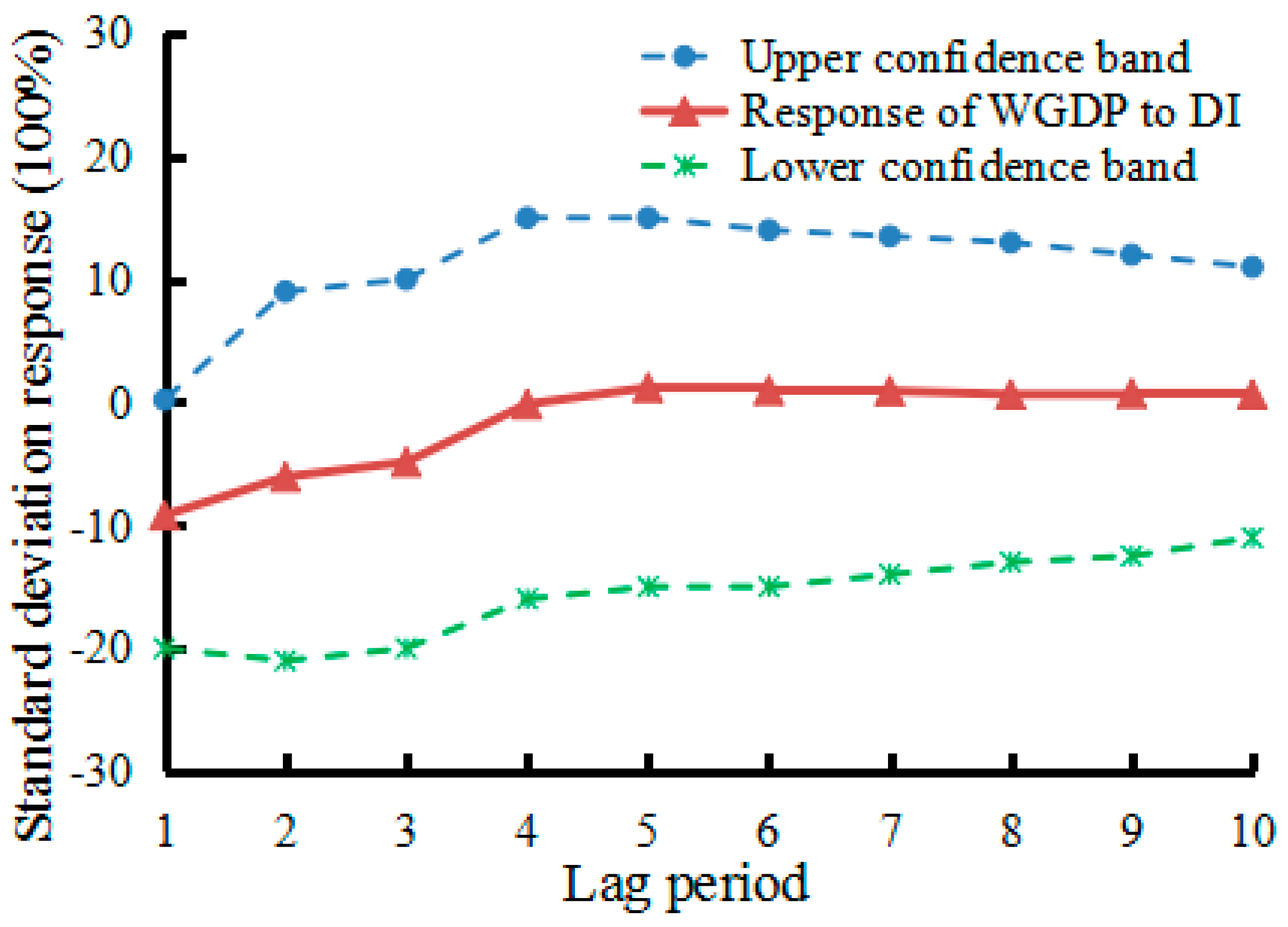
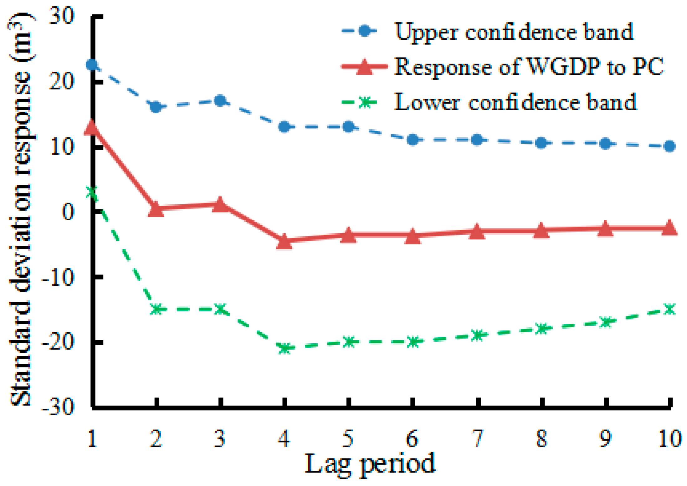
Based on the above literature illumination, the Jiangsu Province of China will be considered as the case study in this paper, and water consumption per ten thousand dollar GDP (WC/$10⁴ GDP) indicates the comprehensive water use efficiency. Then the influencing factors of WC/$10⁴ GDP in Jiangsu Province will be identified under the consideration of Jiangsu industrial development level and the different patterns and characteristics of agricultural, industrial and domestic water consumption. At last, we analyze the relationships between influencing factors and WC/$10⁴ GDP for supporting government decision making. Because some influencing factors such as surface water resources (SW), groundwater resources (GW), precipitation (PT), per capita water resources (PW), per capita water consumption (PC), annual average temperature (AT), drought index (DI), per capita irrigation area (PI) and per capita arable land (PA) cannot be artificially altered, the dynamic system of these natural influencing factors need some input signals to produce the obvious fluctuation (output) to explore the subtle changes. As such, the impulse response is employed in this paper to describe the reaction of the real world system as a function of the independent variables of resource factors that parameterizes the dynamic behavior. Then the VAR model is used to generalize the univariate autoregressive model (AR model) by introducing all the resource factors to investigate their effectiveness.

2. Materials and Methods

Resource factors of WC/$10⁴ GDP in Jiangsu Province indicate the natural endowment, climate change and water resource status always keep steady in the time dimension. Thus, the resource factors can be affected by human activity, but it cannot be artificially manipulated, and that is why we cannot use the multiple regression model to analyze the resource factors. In this paper, we figure out a method of the impulse response function based on vector autoregressive model (VAR) to analyze resource factors. By the method, WC/$10⁴ GDP in Jiangsu Province and its resource factors are put into VAR, then the VAR will give each endogenous variable a unit of standard deviation. As such, we can judge the effect of resource factors through impulse response function.

2.1. Vector Autoregressive Model (VAR)

Vector auto regression model is built based on the data’s statistical properties without the consideration of relationships between phenomena and economic theory basis. VAR is often used for the prediction of multivariable time series system and the dynamic influence of the random disturbance on the variable system. VAR is the generalization of the single variable auto regression model considering that every endogenous variable is the lag value of all the variables in the system [22]. As such, the mathematical expression of VAR model is shown in the following:

$$Y_t={\mathsf{\phi }}_1{Y}_{t-1}+\cdots +{\mathsf{\phi }}_p{Y}_{t-p}+H{X}_t+{\mathsf{\epsilon }}_{t}t=1,2,\cdots ,T$$

(1)

In the expression, Y_t is k-dimensional column vector of endogenous variable; X_t is d-dimensional column vector of exogenous variable; p is the order of the lag; and T is the number of samples. k × k dimensional matrix ${\mathsf{\phi }}_1,\cdots ,{\mathsf{\phi }}_p$ and k × d dimensional matrix H is the coefficient matrix to be estimated. ε_t is k-dimensional perturbed column vector, and Equation (1) can be expanded:

$$\left[\begin{array}{c}{y}_{1t}\\ y_{2t}\\ ⋮\\ y_{kt}\end{array}\right]={\mathsf{\phi }}_1\left[\begin{array}{c}{y}_{1t-1}\\ y_{2t-1}\\ ⋮\\ y_{kt-1}\end{array}\right]+\cdots +{\mathsf{\phi }}_p\left[\begin{array}{c}{y}_{1t-p}\\ y_{2t-p}\\ ⋮\\ y_{kt-p}\end{array}\right]+H\left[\begin{array}{c}{x}_{1t}\\ x_{2t}\\ ⋮\\ x_{dt}\end{array}\right]+\left[\begin{array}{c}{\mathsf{\epsilon }}_{1t}\\ {\mathsf{\epsilon }}_{2t}\\ ⋮\\ {\mathsf{\epsilon }}_{kt}\end{array}\right]$$

(2)

Equation (2) is called the non-restricted vector autoregressive model. Simplified form of impact vector ε_t is white noise vector. For the sake of convenience, the VAR model considered is a non-restricted vector autoregressive model without constant term, shown in the following:

$$Y_t={\mathsf{\phi }}_1{Y}_{t-1}+\cdots +{\mathsf{\phi }}_p{Y}_{t-p}+{\mathsf{\epsilon }}_t$$

(3)

2.2. Time Series Stability Test

The stability of time series is a prerequisite for the establishment of VAR model. When the stability condition is not satisfied [23], it is easy to produce the result of false regression. Hence, the stability of each sequence in the model must be tested first when the VAR model fitting is conducted for the WC/$10⁴ GDP and its factors. Only when the sequence is stable, can we use the VAR model to fit the dynamic regression relation between the sequences. At present, there are many methods to test the stability of unit root, such as DF test, ADF test, PP test and so on. The ADF test is used in this paper, the basic theory can be explained as follows:

For any one VAR (P) process, the expression equation is

$$X_t={\mathsf{\phi }}_1{X}_{t-1}+\cdots +{\mathsf{\phi }}_p{X}_{t-p}+{\mathsf{\epsilon }}_t$$

(4)

The characteristic equation of VAR is ${\mathsf{\lambda }}^p-{\mathsf{\phi }}_1{\mathsf{\lambda }}^{p-1}-\cdots -{\mathsf{\phi }}_p=0$, When all the characteristic roots of the characteristic equation are in the unit circle, namely $\left|{\mathsf{\lambda }}_i\right|$ < 1, i = 1, 2, ..., p, we think the sequence $\{X_t\}$ is stable. Else, if ${\mathsf{\lambda }}_1=1$, we consider the sequence $\{X_t\}$ is unstable, so the sum of the auto-regression coefficients of the equation is just 1, namely:

$${\mathsf{\lambda }}^p-{\mathsf{\phi }}_1{\mathsf{\lambda }}^{p-1}-\cdots -{\mathsf{\phi }}_p=0\stackrel{\mathsf{\lambda }=1}{\Rightarrow }1-{\mathsf{\phi }}_1-\cdots -{\mathsf{\phi }}_p=0\Rightarrow {\mathsf{\phi }}_1+{\mathsf{\phi }}_2+\cdots {\mathsf{\phi }}_p=1$$

(5)

That is to say, the stability of the sequence can be judged by that whether the sum of the coefficients of the equation is 1.

Equivalent transformation of Equation (5) is shown in the following:

$$\begin{array}{lll}{X}_t-X_{t-1}& =& {\mathsf{\phi }}_1{X}_{t-1}+\cdots {\mathsf{\phi }}_p{X}_{t-p}-X_{t-1}+{\mathsf{\epsilon }}_t\\ & =& \begin{array}{c}({\mathsf{\phi }}_2+\cdots {\mathsf{\phi }}_p)\end{array}{X}_{t-1}+{\mathsf{\phi }}_1{X}_{t-1}-X_{t-1}-({\mathsf{\phi }}_2+\cdots {\mathsf{\phi }}_p)X_{t-1}\\ & & +{\mathsf{\phi }}_2{X}_{t-2}+({\mathsf{\phi }}_3+\cdots {\mathsf{\phi }}_p)X_{t-2}-({\mathsf{\phi }}_3+\cdots {\mathsf{\phi }}_p)X_{t-2}\\ & & +{\mathsf{\phi }}_3{X}_{t-3}+({\mathsf{\phi }}_4+\cdots {\mathsf{\phi }}_p)X_{t-3}-({\mathsf{\phi }}_4+\cdots {\mathsf{\phi }}_p)X_{t-3}\\ & & +\cdots -{\mathsf{\phi }}_p{X}_{t-p+1}+{\mathsf{\phi }}_p{X}_{t-p}+{\mathsf{\epsilon }}_t\end{array}$$

(6)

In addition, Equation (6) is:

$$\nabla X_t=({\mathsf{\phi }}_1+\cdots +{\mathsf{\phi }}_p-1)X_{t-1}-({\mathsf{\phi }}_2+\cdots +{\mathsf{\phi }}_p)\nabla X_{t-1}-\cdots -{\mathsf{\phi }}_p\nabla X_{t-p+1}+{\mathsf{\epsilon }}_t$$

(7)

If ${\mathsf{\phi }}_1+{\mathsf{\phi }}_2+\cdots {\mathsf{\phi }}_p-1=\mathsf{\rho }$, and $-({\mathsf{\phi }}_{j+1}+\cdots +{\mathsf{\phi }}_p)={\mathsf{\beta }}_j,j=1,2,\cdots p-1,$ then Equation (7) can be simplified as:

$$\nabla X_t=\mathsf{\rho }{X}_{t-1}+{\mathsf{\beta }}_1\nabla X_{t-1}+\cdots +{\mathsf{\beta }}_{p-1}\nabla X_{t-p+1}+{\mathsf{\epsilon }}_t$$

(8)

If the sequence of $\{X_t\}$ is stable, then ${\mathsf{\phi }}_1+{\mathsf{\phi }}_2+\cdots {\mathsf{\phi }}_p$ < 1, namely, ρ < 0; if $\{X_t\}$ is unstable, there is at least one unit root to make ${\mathsf{\phi }}_1+{\mathsf{\phi }}_2+\cdots {\mathsf{\phi }}_p=1$, namely, ρ = 0. Therefore, the hypothesis of unit root test in the VAR (p) process can be expressed as:

$$H_0:\mathsf{\rho }=0\leftrightarrow H_1:\mathsf{\rho }<0$$

(9)

Then, we construct ADF test statistical quantity:

$$ADF=\frac{\stackrel{\wedge }{\mathsf{\rho }}}{S(\stackrel{\wedge }{\mathsf{\rho }})}$$

(10)

In Equation (10), $S(\stackrel{\wedge }{\mathsf{\rho }})$ is the sample standard deviation of parameter p.

2.3. Determination of the Lag Order

The lag order of the VAR model has great influence on the model’s stability, if lag order is too large, there will be too many parameters the need to be estimated, reducing the degree of freedom and the accuracy of the model. Furthermore, it is not conducive to the model estimation. Therefore, the appropriate lag orders must be determined according to a certain criterion in the process of building the VAR model.

EViews (Econometric Views) software is a statistical package for Windows, used mainly for time-series oriented econometric analysis. Version 1.0 of EViews was released in March 1994, and the software and programming language was originally developed by Robert Hall in 1965 [24]. EViews can be used for general statistical analysis, such as cross-section and panel data analysis and time series estimation and forecasting. EViews combines spreadsheet and relational database technology with the traditional tasks found in statistical software, and uses a Windows GUI. In sum, EViews is a professional tool in the field of statistics, and VAR model is a mature function in it. As such, this paper uses EViews software to build VAR model, in which the VAR module provides several guidelines for the selection of the number of lags.

2.3.1. LR Test Criteria

LR likelihood ratio test is divided into two types: unconstrained model and constrained model. The unconstrained model is the model without any restriction, and the constrained model is the model under the null hypothesis. Two times difference of the maximum likelihood function between the two models is the likelihood ratio (LR) statistical quantity, calculated mode is:

$$LR=2(\stackrel{\wedge }{l_u}-\stackrel{\wedge }{l_r}),{\mathsf{\chi }}^2(k)$$

(11)

where $\stackrel{\wedge }{l_u}$ and $\stackrel{\wedge }{l_r}$ are the maximum value of the likelihood function under the condition of unconstrained and constrained, respectively. A likelihood ratio based method is constructed to obey the chi square distribution statistics, k is the degree of freedom of the chi square distribution, and the number of freedom is equal to the number of the constraint conditions. The test criterion is used to test the validity of the parameter constraints, if the parameter constraints are valid and sufficient, then the constraint should not cause a large decrease in the maximum of the likelihood function. It is proven that the greater the value of the LR, the more insufficient the model constraints.

2.3.2. FPE Test Criteria

The basic idea of FPE test criteria is to use the model one-step prediction error variance to determine whether the autoregressive model is applicable. The smaller the variance of one-step prediction error is, the better the model fitting is. Definition of FPE test criteria:

$$FP{E}_p=\stackrel{\wedge }{{\mathsf{\sigma }}^2}\frac{(n+p)}{(n-p)}$$

(12)

In Equation (12), the coefficient of $\frac{(n+p)}{(n-p)}$ will increase with the increase of p. Along with the increase of the order, residual variance of VAR model $\stackrel{\wedge }{{\mathsf{\sigma }}^2}$ decreases with the increase of p, then if p > p₀, $\stackrel{\wedge }{{\mathsf{\sigma }}^2}$ will not be reduced again, at this time, $\frac{(n+p)}{(n-p)}$ will takes the lead in equation. Ultimately, the p that takes the minimum value of the FPE_p can be determined as the optimal order of the model. The lower lag order number easily makes the model structure shift, and the higher lag order number easily causes the increase of variance, while the FPE criterion can effectively avoid these two kinds of risks, and achieve a kind of balance.

2.3.3. Information Criterion

In the analysis process of VAR model, in order to describe the dynamic characteristics of the structure more completely, the lag period of the model is generally made long enough. However, the lag cannot be too long because the long lag phase will cause the reduction of degrees of freedom. Hence, in practical analysis, it is usually determined according to AIC and SC and HQ information criterion. This can be calculated as follows:

$$\{\begin{array}{l}AIC=-2l/n+2k/n,\hfill \\ SC=-2l/n+k\log n/n,\hfill \\ HQ=-2l/n+2k\log \left(\log \right(n\left)\right)/n,\hfill \end{array}$$

(13)

In Equation (13), $k=m(rd+pm)$ is the number of estimated parameters; n is the number of observations; and $l=-\frac{nm}{2}(1+\log 2\mathsf{\pi })-\frac{n}{2}\log \left[\det ({\displaystyle {\sum }_t\stackrel{\wedge }{{\mathsf{\epsilon }}_t}}\stackrel{\wedge }{{\mathsf{\epsilon }}_t}\prime /n)\right]$.

2.4. Impulse Response Function

In the course of this study, the resource factors do not change with the subjective will of the people due to their characteristics. Thus, in the course of the study, we cannot change the independent variable to analyze its influence effect; instead, we should analyze the model’s dynamic effects when an error to change, or the model is subjected to some kind of impact. Furthermore, this analysis method based on the VAR model is called impulse response function.

For the VAR model, a very important aspect is the dynamic characteristics of the system. When endogenous variable i is given a shock, the impact of shock will not affect the variable i itself. Furthermore, due to the dynamic characteristics of the VAR model, other endogenous variables will be affected by the impact. The impulse response function attempts to describe the trajectory of the impact, and shows how the volatility can affect other variables through the model.

Through the dual variable VAR (Equation (2)) model, the basic theory of the impulse response function is expressed in the following.

$$\{\begin{array}{c}{x}_t=a_1{x}_{t-1}+a_2{x}_{t-2}+b_1{z}_{t-1}+b_2{z}_{t-2}+{\mathsf{\epsilon }}_{1t}\\ z_t=c_1{x}_{t-1}+c_2{x}_{t-2}+d_1{z}_{t-1}+d_2{z}_{t-2}+{\mathsf{\epsilon }}_{2t}\end{array},t=1,2,\dots ,T.$$

(14)

In the above, $a_i,b_i,c_i,d_i$ are parameters, and ${\mathsf{\epsilon }}_t=({\mathsf{\epsilon }}_{1t},{\mathsf{\epsilon }}_{2t})\prime$ is disturbance term. Assuming the disturbance term is white noise vector, its properties are shown as follows:

$$\{\begin{array}{l}E({\mathsf{\epsilon }}_t)=0,\forall t\hfill \\ \mathrm{var}({\mathsf{\epsilon }}_t)=E({\mathsf{\epsilon }}_t{\mathsf{\epsilon }}_t\prime )={\displaystyle \sum },\forall t\hfill \\ E({\mathsf{\epsilon }}_t{\mathsf{\epsilon }}_s\prime )=0,\forall t\ne s\hfill \end{array}$$

(15)

Assuming the system starts from the zeroth phase, so $x_{-1}=x_{-2}=z_{-1}=z_{-2}=0$, and disturbance term ${\mathsf{\epsilon }}_{10}=1,{\mathsf{\epsilon }}_{20}=0$, others are zeros, namely, ${\mathsf{\epsilon }}_{1t}={\mathsf{\epsilon }}_{2t}=0(t=1,2,\dots )$; this process is referred to as the zeroth phase of the X to pulse.

When t = 0: $x_0=1,z_0=0$.

Substituting the results into Equation (14), then while t = 1: $x_1=a_1,z_1=c_1$.

Substituting the results into Equation (14) again, while t = 2:

$$x_2=a_1^2+a_2+b_1{c}_1,z_2=c_1{a}_1+c_2+d_1{c}_1$$

(16)

After continuous substitution, we could get $x_0,x_1,x_2,x_3,x_4$; this process is called the response function of x caused by the impulse of X. In addition, we could get $z_0,z_1,z_2,z_3,z_4$, which is called the z response function caused by the X impulse.

3. Calculation and Results

3.1. Resource Factors Screening

In this paper, the original data are composed of statistical data in Jiangsu Province from 1997 to 2012. Related data are from statistical yearbook of Jiangsu Province, water resources bulletin in Jiangsu Province, China’s Meteorological Administration and China’s Statistical Yearbook. The influencing factors of WC/$10⁴ GDP are shown in

Table 1. Influencing factors’ structure table of WC/$10⁴ GDP.

Dependent Variable	Main Types	Influencing Factors
WC/$104 GDP	Population factors	Urbanization (UZ), Population(TP);
	Resources factors	Surface water resources (SW), groundwater resources (GW), precipitation (PT), per capita water resources (PW), water consumption per capita (PC), annual average temperature (AT), drought index (DI), per capita irrigation area (PI), and per capita arable land (PA);
	Economic factors	Primary industry output value accounted for the proportion of GDP (PG), the tertiary industry accounted for the GDP (TG), industrial output value accounted for the proportion of GDP (IG), food crop area accounted for the proportion of the total sown area of agriculture (FA), high consumption of water industry output value accounted for the proportion of total industrial output value of (HA);
	Technology factors	The standard rate of industrial wastewater discharge (ID), water-saving irrigation area (SI), the expenditure of large and medium-sized industrial enterprises R&D funds accounted for the proportion of main business income (MA), high-tech output value accounted for the proportion of total production value (HI);
	Management factors	Water price (TF), the proportion of expenditure on education expenditure (EF), science and technology expenditures accounted for the proportion of financial expenditure (SF).

according to expert seminar. Then, the data of resource factors of WC/$10⁴ GDP are shown in

Table 2. Data aggregation (resource factors) of WC/$10⁴ GDP influencing factors in Jiangsu from 1997 to 2012.

Years	SW (108 m3)	GW (108 m3)	PT (mm)	PW (m3)	PC (m3)	AT (°C)	DI (100%)	PI (ha)	PA (ha)
1997	159.69	122.05	854.0	360.18	723.00	10.4	3.57	0.81	622.3
1998	379.33	156.38	1186.9	698.99	585.00	10.5	1.68	0.81	619.4
1999	316.84	118.79	1016.8	573.95	610.00	10.5	4.82	0.81	701.7
2000	319.26	143.31	1080.7	585.55	600.00	9.8	4.12	0.80	690.8
2001	181.41	115.31	870.0	357.86	634.00	9.7	4.09	0.79	687.8
2002	185.72	100.59	922.2	361.92	649.00	10.6	4.55	0.79	683.5
2003	499.81	138.28	1255.8	830.08	585.00	10.5	4.79	0.77	678.7
2004	132.43	90.97	784.3	271.20	707.00	10.8	2.60	0.77	672.8
2005	366.38	122.23	1084.0	615.37	697.00	9.8	2.88	0.75	667.1
2006	314.70	110.73	1021.2	528.24	727.00	10.1	3.48	0.75	661.1
2007	395.71	123.27	1089.0	641.84	736.00	11	2.96	0.74	616.8
2008	280.86	111.34	994.3	486.96	730.00	10.9	2.80	0.74	613.7
2009	306.05	110.80	1031.7	512.54	713.00	10.5	3.62	0.73	610.0
2010	291.20	108.90	989.5	487.33	704.00	9.4	2.35	0.73	605.4
2011	399.00	115.10	1012.1	623.39	705.00	10.1	3.27	0.73	603.1
2012	279.10	110.20	953.9	471.34	698.00	10.3	2.84	0.74	601.5

.

3.2. Establishment of Vector Autoregressive Model (VAR)

3.2.1. Selection of Indicators by Correlation Analysis

There exist correlations between the resource factors affecting the WC/$10⁴ GDP in Jiangsu Province. In the process of establishing a vector autoregressive model for the resource factors and the WC/$10⁴ GDP, the number of influencing resource indicators is 9, so the correlation analysis is adopted to delete the number of indicators. In this paper, the correlation analysis is conducted by SPSS software [25]. Software processing results are shown in

Table 3. Output results of correlation coefficient.

Coefficient	SW	GW	PT	PW	PC	AT	DI	PI	PA
SW	1	0.609 *	0.933 **	0.981 **	−0.276	−0.004	0.016	−0.281	−0.144
GW	0.609 *	1	0.762 **	0.734 **	−0.635 **	−0.101	−0.029	0.427	0.042
PT	0.933 **	0.762 **	1	0.968 **	−0.458	0.011	0.03	−0.061	−0.033
PW	0.981 **	0.734 **	0.968 **	1	−0.406	0.008	0.045	−0.104	−0.066
PC	−0.276	−0.635 **	−0.458	−0.406	1	0.149	−0.401	−0.676 **	−0.577 *
AT	−0.004	−0.101	0.011	0.008	0.149	1	−0.001	0.049	−0.112
DI	0.016	−0.029	0.03	0.045	−0.401	−0.001	1	0.352	0.671 **
PI	−0.281	0.427	−0.061	−0.104	−0.676 **	0.049	0.352	1	0.598 *
PA	−0.144	0.042	−0.033	−0.066	−0.577 *	−0.112	0.671 **	0.598 *	1

Notes: * Significant correlation at 0.05 level (bilateral); ** Significant correlation at 0.01 level (bilateral).

.

According to Table 3, SW (surface water) has strong correlation with GW (groundwater), PT (precipitation), and PW (per capita water resources) at 0.05 and 0.01 level (bilateral). After analysis, it is not difficult to find that these four indicators reflect the direct or indirect characterization of the water resources endowment. Surface water (SW) and groundwater (GW) and precipitation (PT) are resource indicators reflecting the water resource distribution among regions of China from the point of view of nature, but these three indicators cannot represent the impact of human activities on natural resources. On the contrary, per capita water resources (PW) can link natural factors with social economic factors, because the calculation method of PW is water resources amount divided by population. Thus, PW involves water resources and population, and the relationship between nature and society are integrated to reflect the influence of human activities on the distribution of water resources. After comprehensive consideration of the four indicators SW, GW, PT, and PW, we choose per capita water resources (PW) to reflect the comprehensive influence of water resources and population removing SW, GW, PT.

Then, the correlation coefficient of PC and PI is −0.676, and the correlation coefficient of PC and PA is −0.577, and they are significantly correlated at 0.01 and 0.05 level (bilateral). The correlation coefficient of PA and DI is 0.671, and they are significantly correlated at the 0.01 level (bilateral). Because of their different definitions, these indicators are all retained.

The correlation coefficient of PI and PA is 0.598, and they are significantly correlated at 0.05 level (bilateral). On the other hand, irrigated area belongs to the cultivated land area; hence, for better characterization of population and land resources, PA index is chosen for analysis, removing PI.

To sum up, five indicators of PW, AT, DI, PC, and PA are finally selected to characterize the resource influencing factors of WC/$10⁴ GDP in Jiangsu Province.

3.2.2. Time Series Stability Test

The stationarity of time series is the premise of establishing the vector auto regressive model, and the EViews software is applied in this article to test the stability of time series.

This paper selects Augmented Dickey–Fuller (ADF) method to test the stability of time series. Output result of Augmented Dickey–Fuller unit root test on annual average temperature (AT) is in

Table 4. Augmented Dickey–Fuller Unit Root Test on AT.

Augmented Dickey–Fuller	Test	Statistic	t-Statistic	Prob. *
			−3.915755	0.0128
Test critical values	1.0%	level	−4.057910
	5.0%	level	−3.119910
	10%	level	−2.701103

Notes: * Probability: a number between 0 and 1 measuring the likelihood that an event will occur.

.

Under the original hypothesis, $H_0:\mathsf{\rho }=0\leftrightarrow H_1:\mathsf{\rho }<0$, the unit root t test statistic value is −3.916. Then, the critical values of the unit root test are −4.058, −3.120, and −2.701, respectively, at 1%, 5%, and 10% significant levels. Obviously, the value of the t test statistic is less than the critical values at 10% and 5% significant levels, and the Probability value is less than 0.05, hence AT (average temperature) in the time series is stable.

Respectively conducting the unit root test of the remaining four indicators and WC/$10⁴ GDP in Jiangsu Province, the results show that PW, DI, PC, and WC/$10⁴ GDP in Jiangsu are stable in time series. PA is not stable in time series. Thus, we tackle the PA index by first order difference to characterize the fluctuation change of PA, expressed as DPA index. Through the unit root test, DPA is stable. As such, the EViews output is shown in

Table 5. VAR stability condition check.

Variables	Unit	Root	Modulus (Positive Value)
DPA	ha	0.900119	0.900119
DI	100%	0.599834	0.599834
AT	°C	−0.513577 − 0.076426i	0.519232
PC	m3	−0.513577 + 0.076426i	0.519232
WGDP	m3/104 dollar	0.260554 − 0.390520i	0.469467
PW	m3	0.260554 + 0.390520i	0.469467

.

In statistics, a unit root test tests whether a time series variable is non-stationary and possesses a unit root, if there is a unit root in the test sequence, the variable is a non-stationary time series. A commonly used test that is valid in large samples is the augmented Dickey–Fuller test. If the root’s modulus is less than 1.0 after augmented Dickey–Fuller test, it means the time series variable is stationary. The augmented Dickey–Fuller test is applied in this paper, and the variables of DPA, DI, AT, PC, WGDP, and PW are stationary because all the roots’ modulus are less than 1.0 (Table 5).

3.2.3. Determination of the Lag Order

In this paper, we use the non-constrained VAR model, i.e. the parameters are not null constraint, all of which are left in the equation. Considering there are too many variables in this paper, the estimated time lag interval is one order. Lag order judgment result is shown in

Table 6. Lag order judgment result.

Lag	LogL	LR	FPE	AIC	SC	HQ
0	−284.6522	NA	1.06 × 1012	44.71573	44.97647	44.66213
1	−199.8732	78.25756 *	1.25 × 109 *	37.21 *	39.03648	36.8361
2	1993.296	0	NA	NA	−291.2712 *	−295.3576 *

Notes: * indicates lag order selected by the criterion. LR: sequential modified LR test statistic (each test at 5% level); FPE: Final prediction error; AIC: Akaike information criterion; SC: Schwarz information criterion; HQ: Hannan–Quinn information criterion. NA: Not Applicable.

.

More than half of the lag orders are one-order, so the lag order of VAR model is one.

3.2.4. VAR Parameters Estimation

After the establishment of VAR model, we need to ensure the VAR parameters, including the results of the model parameter estimation, standard deviation of the estimated coefficient, and t test statistic values. Results of model output are shown in

Table 7. VAR model parameters estimated value output.

Parameters Value	AT	DI	DPA	PC	WGDP	PW
AT (−1)	0.046864	−0.265183	14.64371	−11.71337	−5.770008	32.28154
	(−0.34302)	(−0.37699)	(−8.07601)	(−20.2873)	(−12.7095)	(−89.6439)
	[0.13662]	[−0.70342]	[1.81324]	[−0.57737]	[−0.45399]	[0.36011]
DI (−1)	0.100744	−0.155794	−23.82463	2.279396	−12.39079	−33.63872
	(−0.19236)	(−0.21141)	(−4.5288)	(−11.3766)	(−7.12712)	(−50.2698)
	[0.52374]	[−0.73694]	[−5.26069]	[0.20036]	[−1.73854]	[−0.66916]
DPA (−1)	−0.008511	−0.000509	−0.020488	−0.320118	0.125379	1.483916
	(−0.00688)	(−0.00757)	(−0.16209)	(−0.40718)	(−0.25509)	(−1.79921)
	[−1.23623]	[−0.06728]	[−0.12640]	[−0.78618]	[0.49151]	[0.82476]
PC (−1)	0.004549	0.000254	−0.46946	0.523744	−0.228322	1.211876
	(−0.00731)	(−0.00804)	(−0.1722)	(−0.43257)	(−0.271)	(−1.91142)
	[0.62198]	[0.03158]	[−2.72625]	[1.21076]	[−0.84253]	[0.63402]
WGDP (−1)	0.001519	0.004311	−0.02566	−0.090203	0.89556	0.304307
	(−0.00225)	(−0.00248)	(−0.05303)	(−0.1332)	(−0.08345)	(−0.58858)
	[0.67451]	[1.74171]	[−0.48393]	[−0.67719]	[10.7320]	[0.51702]
PW (−1)	0.001422	−0.00109	−0.008391	0.126037	0.087052	−0.295979
	(−0.00146)	(−0.00161)	(−0.03445)	(−0.08653)	(−0.05421)	(−0.38237)
	[0.97170]	[−0.67791]	[−0.24358]	[1.45649]	[1.60578]	[−0.77406]
C	5.127786	5.7772	257.1599	401.1283	208.0335	−442.4652
	(−6.0279)	(−6.62493)	(−141.92)	(−356.511)	(−223.345)	(−1575.32)
	[0.85068]	[0.87204]	[1.81200]	[1.12515]	[0.93144]	[−0.28087]
R2	0.283881	0.707515	0.865725	0.780159	0.99085	0.414763
Adj. R2	−0.329936	0.456813	0.750632	0.591724	0.983008	−0.086869

.

In Table 7, the standard deviations of estimated coefficients are in parentheses, and t test statistic values are in square brackets. It can be seen that the goodness of fit of the equation of WC/$10⁴ GDP is “R² = 99.1%, adjusted R² = 98.3%”, which is brilliant. The overall fitting degree of the model is of practical significance, so that the impulse response function can be analyzed based on the VAR model.

3.2.5. Impulse Response Function

In this paper, we choose to generate a standard deviation disturbance for five resource factors. Furthermore, the variable of impulse response function is WC/$10⁴ GDP, the definition of impulse is “Generalized Impulses”, this impulse form can overcome the effect of the order of the variables on the results. The results of impulse response are shown in Figure 1, Figure 2, Figure 3, Figure 4 and Figure 5.

In signal processing, the impulse response, or impulse response function (IRF), of a dynamic system is its output when presented with a brief input signal, called an impulse. More generally, an impulse response is the reaction of any dynamic system in response to some external change. Thus, in Figure 1, Figure 2, Figure 3, Figure 4 and Figure 5, the impulse response describes the reaction of the system to the input (standard deviation) of AT, DI, DPA, PC, and PW. The positive square root of the variance is called the standard deviation, and its response can be called standard deviation response of WGDP to variables. Then, the confidence band is used in statistical analysis to represent the uncertainty in an estimate of a curve or function based on limited or noisy data. Confidence bands are used as part of the graphical presentation of results of a regression analysis in this paper.

4. Generalized Error Variance Decomposition

In econometrics and other applications of multivariate time series analysis, a variance decomposition or forecast error variance decomposition (FEVD) is used to aid in the interpretation of a vector autoregression (VAR) model once it has been fitted. The variance decomposition indicates the amount of information each variable contributes to the other variables in the autoregression. It determines how much of the forecast error variance of each of the variables can be explained by exogenous shocks to the other variables. After calculation, the variance decomposition of WGDP is shown in

Table 8. Variance decomposition of WGDP (%).

Period	S.E.	AT	DI	DPA	PC	PW	WGDP
1	20.72106	0.581717	20.23531	0.017695	24.8321	48.74403	5.589146
2	23.1208	6.363611	19.5115	1.005327	21.80245	43.22754	8.08957
3	26.1667	6.250065	17.57603	5.864287	17.02775	44.8133	8.468576
4	28.095	5.42728	15.2548	8.999818	18.88198	42.73912	8.696997
5	29.71585	5.077147	13.69095	11.30537	17.83286	43.37967	8.714001
6	30.87224	4.775345	12.73593	12.51514	17.87449	43.32448	8.77461
7	31.79908	4.540945	12.05792	13.45032	17.41168	43.73291	8.806224
8	32.51921	4.351742	11.5592	14.11376	17.25196	43.88726	8.836091
9	33.10929	4.210524	11.18735	14.64949	17.05155	44.0541	8.846984
10	33.58149	4.101602	10.90331	15.05326	16.9411	44.14698	8.853743

.

S.E. in Table 8 is sampling error. Since sampling is typically done to determine the characteristics of the whole variable, the difference between the sample and the variable’s total information is considered a sampling error.

Table 8 is the generalized error variance decomposition results of WGDP in VAR model, which shows that WGDP’s impulse impact on itself is small, and the five indicators contribute the major information to the variance of WGDP. According to the impulse impact level on WGDP, PW explains the most changes of WGDP, its influence on WGDP ranks first among five indicators. The percent WC/$10⁴ GDP variance due to PW ranges from 48.744% (t = 1) to 44.147% (t = 10). PC ranks second among five indicators, the percent WC/$10⁴ GDP variance due to PC ranges from 24.8321% (t = 1) to 16.9411% (t = 10). DI ranks third among five indicators, the percent WC/$10⁴ GDP variance due to DI ranges from 20.23531% (t = 1) to 10.90331% (t = 10). DPA ranks fourth among five indicators, the percent WC/$10⁴ GDP variance due to DPA ranges from 1.005327% (t = 2) to 15.05326% (t = 10). AT ranks last among five indicators, the percent WC/$10⁴ GDP variance due to AT ranges from 0.581717% (t = 1) to 4.101602% (t = 10). These results are summarized in Figure 6.

5. Discussion

5.1. Interpretation of Results

The solid lines in Figure 1, Figure 2, Figure 3, Figure 4 and Figure 5 express the impulse response of new standard deviation (i.e., new information) caused by AT, DI, DPA, PC and PW on WC/$10⁴ GDP. The dotted lines indicate the confidence band of the standard deviation of the corresponding impulse response image. Impulse response is written in

Table 9. Impulse response results of WC/$10⁴ GDP in Jiangsu Province.

Period	AT	DI	DPA	PC	PW
1	−1.580403	−9.180693	−6.126839	12.98747	−19.46988
2	−5.614299	−6.062402	−0.113568	0.424988	−3.811191
3	−2.962419	−4.852788	2.131412	1.127247	−7.896122
4	0.212443	−0.155034	3.813923	−4.543087	−0.319903
5	1.411991	1.20046	4.099284	−3.579244	−2.316912
6	0.825082	0.970507	3.514161	−3.740345	−1.106128
7	0.635313	0.928108	3.339708	−3.016643	−1.854677
8	0.320056	0.638911	2.950732	−2.850595	−1.39183
9	0.370391	0.7277	2.794542	−2.599934	−1.379167
10	0.312453	0.643254	2.514268	−2.40792	−1.139388

.

It can be seen from the above table that the WC/$10⁴ GDP in Jiangsu Province has certain responses to standard deviation of five factors. For the continuous time of response, it is found that the DPA, PC and PW have longer continuous time effect on WC/$10⁴ GDP. Then, influencing time of AT and DI on WC/$10⁴ GDP is short, the impacts of AT and DI almost disappeared in the 5th period. From the point of view of the strength of the response, the rank of response intensity is: PW > PC > DI > DPA > AT.

5.2. Implications for Similar Research

In this paper, based on the status quo of water resource utilization in Jiangsu Province, the comprehensive water efficiency of Jiangsu province was investigated using the WC/$10⁴ GDP as the water use efficiency index. Furthermore, the government of China planned to find the key factors influencing on water use efficiency, to promote the reasonable utilization of water resources in Jiangsu Province achieving the sustainable development of water resources. By influencing factors determination based on literature research and experts consultation, and data collecting from a variety of channels, the factors of water consumption and index data of Jiangsu Province in 1997–2012 were figured out as the preparation of water use efficiency research. According to the statistical characteristics of index data and the comparison of different mathematical models, this paper applied impulse response function analysis based on vector auto regression model to analyze the impact of resource factors. After case study, it is proved that this model has certain precision and reliability. In addition, it is better to find the main factors that affect the water consumption of GDP in Jiangsu Province. Preliminary analysis on the influencing factors by means of multiple linear regression equation and principal component analysis is quite effective proposed by Jia et al. [26]. However, the multiple linear regression analysis cannot cope with the resource factors because there is a lack of linear relationship. Then, the impulse response analysis based on the vector auto regression model is beneficial to analyze the resource factors, so these two methods can complement each other, which makes the research conclusion more scientific owing theoretical basis. In addition, the reasonable selection of method makes the factors analysis of Jiangsu Province’s water consumption more in line with the actual situation, providing a clear purpose of government regulation and a demonstration for the future water distribution. Taking into account the resource factors which reflect perennial climate characteristics, water reserves, etc. in Jiangsu, we applied correlation analysis to screen the factors first and introduced impulse response function to analyze the final index. It can correctly reflect the relationship between the resource factors and the efficiency of water resources, to identify the significant effect on water use efficiency index.

5.3. Future Research Directions

Due to the limited level of the authors, this paper only studies a part of resource factors of the water consumption to show the significance of mathematical model, and the comprehensiveness research of the assessment indicators is insufficient. The utilization efficiency of water resources is generally affected by factors from various aspects such as economics, policies, and endowment. Furthermore, in the process of index selection, considering the availability of data, some indicators were deleted because of serious lack of statistical data, so that maybe we have ignored a number of important indicators reducing the comprehensiveness of index system. Then the influencing factors of water consumption of Jiangsu Province have been investigated from the macro perspective, and the micro angle research needs to conduct in the future. It is clear that a gap exists between the theoretical exploration and practical application in this paper. That is, we need to further enhance our ability and level of scientific research to link theory with practice, so that the purpose of promoting the application of the conclusions of this paper can be achieved.

Based on expounding the water use efficiency evaluation, it is advised that the expert appraisal and audit to determine the water use efficiency’s driving factors must abide by the rules including comprehensiveness, objectivity, non-overlapping, and easy to obtain. The screening phase is divided into two stages in the following.

• Initial stage is to determine the total goal of evaluation by integrating multiple factors. Namely, the formation of complete index system is according to the logic relationship between the constituent elements of variables.
• Index screening stage is to consult the experts on the preliminary development of the indicators, and according to the feedback, the screening, modification and improvement of index system are conducted to determine the index system ultimately.

6. Conclusions

• Annual average temperature (AT) and drought index (DI) reflect the climatic conditions in Jiangsu Province. As shown in Table 9, the standard deviation response of WC/$10⁴ GDP to AT of 1st period is −1.580403 °C, showing that the AT has a small impact on WC/$10⁴ GDP in the beginning. Then, in the 2nd period, the standard deviation response reaches the peak of −5.61 °C, implying that AT gives a significant influence on WC/$10⁴ GDP. After the 2nd period, the influencing strength of AT decreases gradually, and the standard deviation response become very small after 5th period. For the situation of DI, the standard deviation response of WC/$10⁴ GDP reaches peak of −9.180693 (100%) in the 1st period, and the influencing strength of DI becomes very small after 5th period. To sum up, WC/$10⁴ GDP in Jiangsu Province is sensitive to climate change, once the climatic conditions change, the WC/$10⁴ GDP responds quickly. However, the length of time of impact of AT and DI is relatively short, so we just need to pay attention to their short-term effects. According to Table 8, the percent WC/$10⁴ GDP variance due to DI ranges from 20.23531% (t = 1) to 10.90331% (t = 10), and the percent WC/$10⁴ GDP variance due to AT ranges from 6.363611% (t = 2) to 4.101602% (t = 10). As such, the DI has more influence on WC/$10⁴ GDP, compared with AT, DI is more suitable to reflect the impact of climatic conditions on WC/$10⁴ GDP in Jiangsu Province.
• Per capita water resources index (PW) is based on the data of surface water resources and groundwater resources index, considering the population factor. Furthermore, PW is used to reflect the general situation of water resources in Jiangsu Province. Providing a standard deviation to WGDP by PW, WC/$10⁴ GDP of Jiangsu Province instantly has a significant response, and the variance reaches the peak of −19.47 m³ in 1st period. In addition, the response continues for a long time, illustrating that PW is a very important influencing factor on WC/$10⁴ GDP. Based on the impulse impact level, the influence of PW on WGDP ranks first among five indicators, shown in Table 8. The percent WC/$10⁴ GDP variance due to PW ranges from 48.744% (t = 1) to 44.147% (t = 10). In conclusion, the change of PW is a long-term impact on WC/$10⁴ GDP with a significant intensity, and we need to investigate the mechanism of its effect in the future research.
• It is shown that WC/$10⁴ GDP of Jiangsu Province has not produced obvious fluctuation when the per capita arable land area (DPA) and per capita water consumption (PC) change in Figure 3 and Figure 4. The standard deviation responses of WC/$10⁴ GDP to DPA and PC in the 1st period are −6.126839 and 12.98747 m³, respectively, meaning the initial impact of DPA and PC is obvious. In the 2nd period, the standard deviation responses of WC/$10⁴ GDP to DPA and PC sharply decrease, the figures are only −0.113568 and 0.424988 m³ respectively. However, the impact of DPA and PC on WC/$10⁴ GDP continues for a long time, the standard deviation responses of WC/$10⁴ GDP to DPA and PC change between 2.5 and 4.5 m³ after 4th period. This result shows that we should pay attention to the long-term influence of these two variables in the future. On the other hand, the percent WC/$10⁴ GDP variance due to PC ranges from 24.8321% (t = 1) to 16.9411% (t = 10). Furthermore, the percent WC/$10⁴ GDP variance due to DPA ranges from 1.005327% (t = 2) to 15.05326% (t = 10). That is to say, the impact of PC on WC/$10⁴ GDP is more stationary than DPA.

In summary, as the objective existence, resource factors have an influence that cannot be ignored on WC/$10⁴ GDP in Jiangsu Province. In recent years, sharp economic development in Jiangsu Province has been made the water consumption increase rapidly, and the resource factors have gradually formed the constraints on economic development. Thus, the suggestions for government management are:

• Strengthen the regulation and control of water consumption to ensure reasonable development and utilization of water resources in Jiangsu Province.
• Fully mobilize the subjective initiative of the public to enhance their awareness of saving water and to decrease the emissions of domestic sewage and industrial wastewater.

References

1. Wang, G.F.; Chen, J.C.; Wu, F.; Li, Z.H. An integrated analysis of agricultural water-use efficiency: A case study in the Heihe River Basin in Northwest China. Phys. Chem. Earth 2015, 89–90, 3–9. [Google Scholar] [CrossRef]
2. Dawadi, S.; Ahmad, S. Evaluating the impact of demand-side management on water resources under changing climatic conditions and increasing population. J. Environ. Manag. 2013, 114, 261–275. [Google Scholar] [CrossRef] [PubMed]
3. Pereira, L.S.; Cordery, I.; Iacovides, I. Improved indicators of water use performance and productivity for sustainable water conservation and saving. Agric. Water Manag. 2012, 108, 39–51. [Google Scholar] [CrossRef]
4. Cao, X.C.; Wang, Y.B.; Wu, P.; Zhao, X.N. Water productivity evaluation for grain crops in irrigated regions of China. Ecol. Indic. 2015, 55, 107–117. [Google Scholar] [CrossRef]
5. Scott, C.A.; Vicuna, S.; Blanco-Gutiérrez, I.; Meza, F.; Varela-Ortega, C. Irrigation efficiency and water-policy implications for river basin resilience. Hydrol. Earth Syst. Sci. Discuss. 2014, 18, 1339–1348. [Google Scholar] [CrossRef] [Green Version]
6. Cao, X.; Wu, P.; Wang, Y.; Zhao, X. Water footprint of grain product in irrigated farmland of China. Water Resour. Manag. 2014, 28, 2213–2227. [Google Scholar] [CrossRef]
7. Cao, X.; Wu, P.; Wang, Y.; Zhao, X. Assessing blue and green water utilization in wheat production of China from the perspectives of water footprint and total water use. Hydrol. Earth Syst. Sci. Discuss. 2014, 18, 3165–3178. [Google Scholar] [CrossRef] [Green Version]
8. Abd El-Wahed, M.H.; Ali, E.A. Effect of irrigation systems, amounts of irrigation water and mulching on corn yield, water use efficiency and net profit. Agric. Water Manag. 2013, 120, 64–71. [Google Scholar] [CrossRef]
9. Wang, M.; Shao, G.; Meng, J.; Chen, C. Variable fuzzy assessment of water use efficiency and benefits in irrigation district. Water Sci. Eng. 2015, 8, 205–210. [Google Scholar] [CrossRef]
10. Li, M.; Guo, P.; Singh, V.P. An efficient irrigation water allocation model under uncertainty. Agric. Syst. 2016, 144, 46–57. [Google Scholar] [CrossRef]
11. García-Bolanos, M.; Borgia, C.; Poblador, N.; Dia, M.; Seyid, O.M.V.; Mateos, L. Performance assessment of small irrigation schemes along the Mauritanian banks of the Senegal River. Agric. Water Manag. 2011, 98, 1141–1152. [Google Scholar] [CrossRef]
12. Peng, S.; Luo, Y.; Xu, J.; Shahbaz, K.; Jiao, X.; Wang, W. Integrated irrigation and drainage practices to enhance water productivity and reduce pollution in a rice production system. Irrig. Drain. 2012, 61, 285–293. [Google Scholar] [CrossRef]
13. Fan, Y.; Wang, C.; Nan, Z. Comparative evaluation of crop water use efficiency, economic analysis and net household profit simulation in arid Northwest China. Agric. Water Manag. 2014, 146, 335–345. [Google Scholar] [CrossRef]
14. Wang, W.; Yu, Z.; Zhang, W.; Shao, Q.; Zhang, Y.; Luo, Y.; Jiao, X.; Xu, J. Responses of rice yield, irrigation water requirement and water use efficiency to climate change in China: Historical simulation and future projections. Agric. Water Manag. 2014, 146, 249–261. [Google Scholar] [CrossRef]
15. Ma, Y.; Feng, S.; Song, X. Evaluation of optimal irrigation scheduling and groundwater recharge at representative sites in the North China Plain with SWAP model and field experiments. Comput. Electron. Agric. 2015, 116, 125–136. [Google Scholar] [CrossRef]
16. Huttona, R.J.; Loveys, B.R. A partial root zone drying irrigation strategy for citrus—Effects on water use efficiency and fruit characteristics. Agric. Water Manag. 2011, 98, 1485–1496. [Google Scholar] [CrossRef]
17. Liu, J.; Sun, S.; Wu, P.; Wang, Y.; Zhao, X. Evaluation of crop production, trade, and consumption from the perspective of water resources: A case study of the Hetao irrigation district, China, for 1960–2010. Sci. Total Environ. 2015, 505, 1174–1181. [Google Scholar] [CrossRef] [PubMed]
18. Sun, S.; Liu, J.; Wu, P.; Wang, Y.; Zhao, X.; Zhang, X. Comprehensive evaluation of water use in agricultural production: A case study in Hetao Irrigation District, China. J. Clean. Prod. 2016, 112, 4569–4575. [Google Scholar] [CrossRef]
19. Sun, S.; Wu, P.; Wang, Y.; Zhao, X.; Liu, J.; Zhang, X. The impacts of interannual climate variability and agricultural inputs on water footprint of crop production in an irrigation district of China. Sci. Total Environ. 2013, 444, 498–507. [Google Scholar] [CrossRef] [PubMed]
20. Ahmadzadeh, H.; Morid, S.; Delavar, M.; Srinivasan, R. Using the SWAT model to assess the impacts of changing irrigation from surface to pressurized systems on water productivity and water saving in the Zarrineh Rud catchment. Agric. Water Manag. 2015, 175, 15–28. [Google Scholar] [CrossRef]
21. Tao, F.; Zhang, Z. Impacts of climate change as a function of global mean temperature: Maize productivity and water use in China. Clim. Chang. 2011, 105, 409–432. [Google Scholar] [CrossRef]
22. Vua, V.H.; Liu, Z.H.; Thomas, M.; Li, W.; Hazel, B. Output-only identification of modal shape coupling in a flexible robot by vector autoregressive modeling. Mech. Mach. Theory 2016, 97, 141–154. [Google Scholar] [CrossRef]
23. Tang, L.; Lv, H.; Yang, F.; Yu, L. Complexity testing techniques for time series data: A comprehensive literature review. Chaos Solitons Fractals 2015, 81, 117–135. [Google Scholar] [CrossRef]
24. Doti James, L.; Esmael, A. Econometric Analysis with MicroTSP Student Software: An Applications Approach; Prentice Hall: Englewood Cliffs, NJ, USA, 1987. [Google Scholar]
25. Alan, B.; Duncan, C. Quantitative Data Analysis with IBM SPSS 17, 18 and 19: A Guide for Social Scientists; Routledge: New York, NY, USA, 2011. [Google Scholar]
26. Jia, R.F.; Fang, S.B.; Tu, W.R.; Sun, Z.L. Driven Factors Analysis of China’s Irrigation Water Use Efficiency by Stepwise Regression and Principal Component Analysis. Discret. Dyn. Nat. Soc. 2016, 2016, 8957530. [Google Scholar] [CrossRef]
Figure 1. Standard deviation response of WGDP to AT.
Water 09 00018 g001
Figure 2. Standard deviation response of WGDP to DI.
Water 09 00018 g002
Figure 3. Standard deviation response of WGDP to DPA.
Water 09 00018 g003
Figure 4. Standard deviation response of WGDP to PC.
Water 09 00018 g004
Figure 5. Standard deviation response of WGDP to PW.
Water 09 00018 g005
Figure 6. Variance decomposition of WGDP.
Water 09 00018 g006