Article

Statistical Analysis of the Spatial Distribution of Multi-Elements in an Island Arc Region: Complicating Factors and Transfer by Water Currents

National Institute of Advanced Industrial Science and Technology, Geological Survey of Japan, Central 7, 1-1-1 Higashi, Tsukuba, Ibaraki 305-8567, Japan
*
Author to whom correspondence should be addressed.
Water 2017, 9(1), 37; https://doi.org/10.3390/w9010037
Submission received: 13 October 2016 / Revised: 23 December 2016 / Accepted: 5 January 2017 / Published: 10 January 2017
(This article belongs to the Special Issue Sediment Transport in Coastal Waters)

Abstract

:
The compositions and transfer processes affecting coastal sea sediments from the Seto Inland Sea and the Pacific Ocean are examined through the construction of comprehensive terrestrial and marine geochemical maps for western Japan. Two-way analysis of variance (ANOVA) suggests that the elemental concentrations of marine sediments vary with particle size, and that this has a greater effect than the regional provenance of the terrestrial material. Cluster analysis is employed to reveal similarities and differences in the geochemistry of coastal sea and stream sediments. This analysis suggests that the geochemical features of fine sands and silts in the marine environment reflect those of stream sediments in the adjacent terrestrial areas. However, gravels and coarse sands do not show this direct relationship, which is likely a result of mineral segregation by strong tidal currents and the denudation of old basement rocks. Finally, the transport processes for the fine-grained sediments are discussed, using the spatial distribution patterns of outliers for those elements enriched in silt and clay. Silty and clayey sediments are found to be transported and dispersed widely by a periodic current in the inner sea, and are selectively deposited at the boundary of different water masses in the outer sea.

1. Introduction

The Geological Survey of Japan, part of the National Institute of Advanced Industrial Science and Technology (AIST), provides nationwide geochemical maps of elements within stream and marine sediments [1]. These geochemical maps have been utilized to explore mineral occurrences and determine the natural abundance of elements, and nationwide and cross-boundary geochemical maps have been developed for such purposes in many countries (e.g., [2,3,4,5,6]). In addition, Japanese geochemical maps have also been created specifically for the purposes of environmental assessment. Ohta and Imai [7] demonstrate an additional use of land and marine geochemical maps, examining particle transfer processes from the land to the sea, or within the marine environment. However, determining provenances with geochemical maps is typically challenging, due to the mixing and homogenization of marine sediments, especially fine sediments such as silt, during transport (e.g., [8]).
In this study, we sought to use geochemical maps of the provenance and transfer analyses of coastal sea sediments in the Chugoku and Shikoku regions, including the Seto Inland Sea and nearby Pacific Ocean as inner and outer seas, respectively (Figure 1a). This region is appropriate for clarifying the influence of terrestrial source materials on the adjacent marine environment, because most rock types found in Japan are distributed in the study area. The Seto Inland Sea is subject to significant tidal variation, while the Pacific Ocean off the Shikoku region is influenced by the Kuroshio Current and the Kuroshio Counter-Current. A number of previous studies of the Seto Inland Sea have analyzed the seafloor topography [9], periodic currents [10], marine organization [11], surface sediments [12], particle transport by marine currents [13,14], and contamination processes [15]. Therefore, this region is well-understood and is considered suitable for investigations into water-current transport processes, especially those between an inner and outer sea. The present study is intended to objectively reveal the complex factors affecting the spatial distributions of elements in coastal sea sediments using various statistical analyses.

2. Geological and Marine Settings

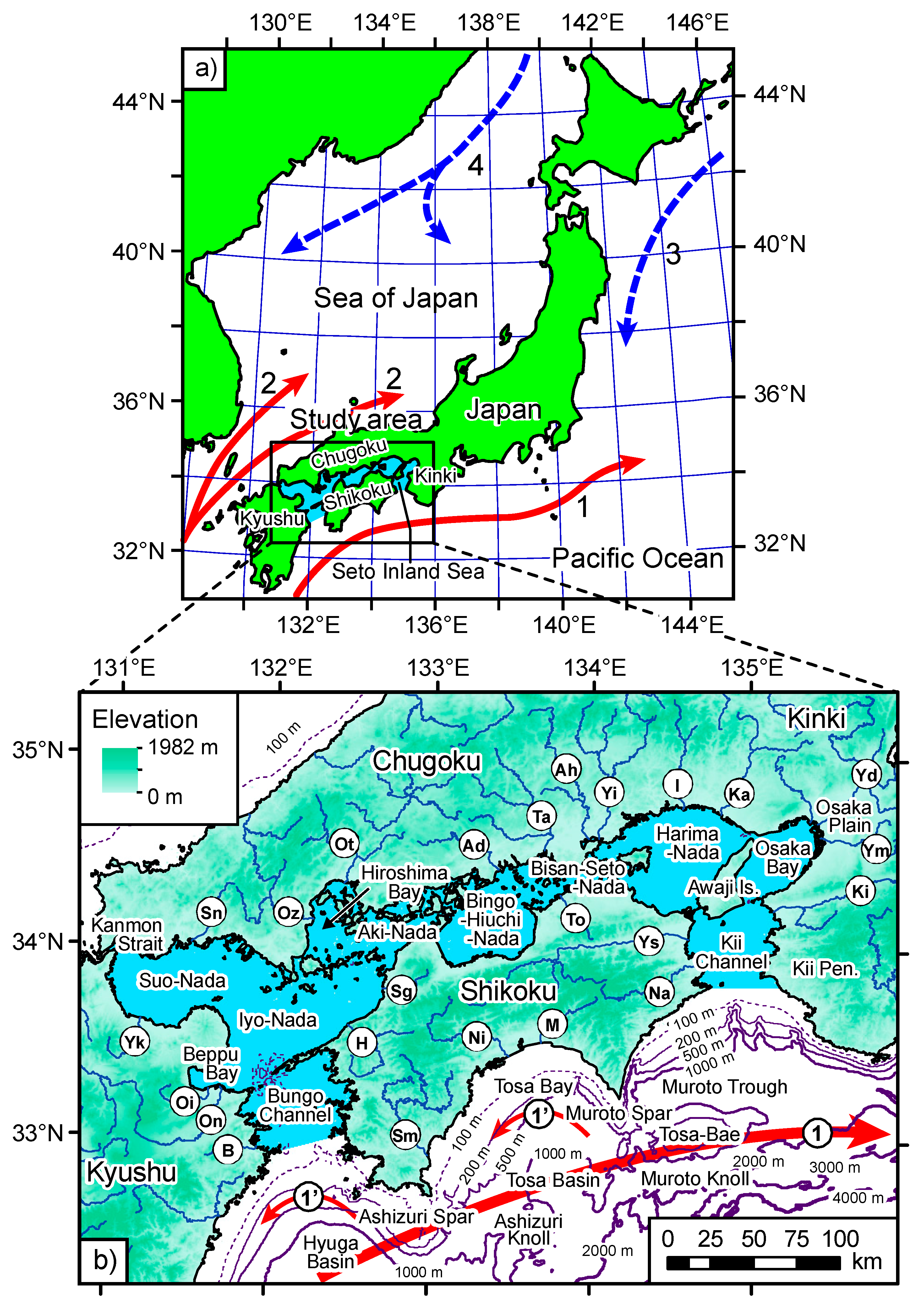
2.1. Riverine System

Figure 1b presents a generalized location map of the study area showing the 24 major rivers. The region is mainly mountainous with small tracts of flat land. The bed slope of the streams on Shikoku Island and the Kii Peninsula is very steep, so rainwater is immediately discharged through the rivers to the sea. Table 1 presents the potential sediment yield from each terrestrial region, which is calculated using the data of Akimoto et al. [16] (Appendix A). Several rivers in the Chugoku and Kyushu regions that flow directly into the Sea of Japan, and from which marine sediments were collected, are not discussed in this study. In this regard, the sediment yield data of these rivers are excluded from Table 1. The Yodo, Yoshino, and Shimanto Rivers are the three largest rivers, each with a high sediment yield (Yd, Ys, and Sm, respectively, in Figure 1b), and the Chugoku, Kinki, Shikoku, and Kyushu regions supply 15%, 5%, 5%, and 1% of the total sediment yield to the Seto Inland Sea, respectively. Therefore, it can be seen that most sediments in the Seto Inland Sea originate from the Chugoku region. The Yodo River flows through several large cities, including Kyoto and Osaka, and discharges into Osaka Bay. Together, the Yodo and Yamato Rivers supply 19% of the total sediment yield to Osaka Bay. Rivers on Shikoku Island are the primary source of sediments to the Pacific Ocean side with 22% of the total sediment yield supplied to Tosa Bay. The Kii Channel also receives a high sediment discharge of 23% from Shikoku Island and the Kii Peninsula. In contrast, little sediment is discharged from rivers into the Bungo Channel.

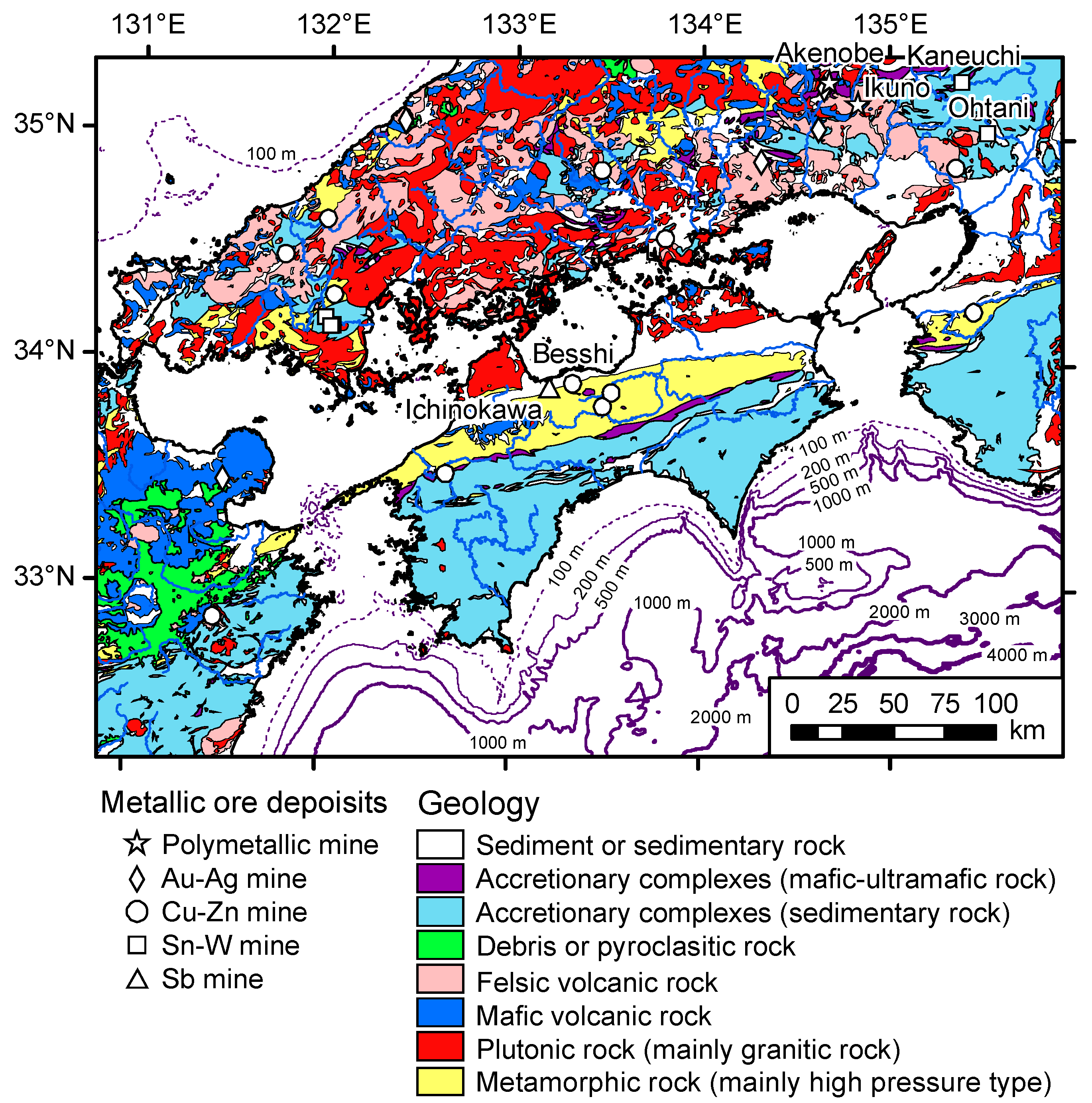
2.2. Geology and Terrestrial Metalliferous Deposits

Figure 2 presents a geological map of the study area, simplified from the Geological Map of Japan 1:1,000,000 [17]. The geology varies considerably between the Chugoku, Kinki, Shikoku, and Kyusyu regions. Rhyolitic-dacitic volcanic rocks and granitic rocks of Cretaceous and Paleogene age are widely distributed in the Chugoku region. In addition, Permian accretionary complexes associated with large limestone blocks, and Triassic high-pressure Sangun metamorphic rocks outcrop in western and central Chugoku. On Shikoku Island, the zonal arrangement of rock units from north to south is as follows: (1) Cretaceous granite-granodiorite; (2) Cretaceous sedimentary rocks; (3) Jurassic–Cretaceous high-pressure Sambagawa metamorphic rocks, comprising quartz schist and greenschist, associated with Mikabu greenstones consisting of basaltic, pyroclastic and ultramafic rocks; and (4) sedimentary rocks of accretionary complexes dated mainly to the Cretaceous-Paleogene. These rock types also outcrop on southern Kyushu Island and on the Kii Peninsula, while andesitic volcanic rocks and debris-pyroclastic rocks of Neogene-Quaternary age extensively outcrop in the northeast of Kyushu Island. Sedimentary rocks of accretionary complexes dating mostly to the Jurassic-Cretaceous outcrop in the northern Kinki region. Unconsolidated Quaternary sediments are restricted in distribution, occurring mainly in the Kinki region. The Osaka Plain is formed of these Quaternary sediments and is the widest plain in the entire study area, with a population of approximately 10 million people.
Figure 2 also shows the locations of some major economic metalliferous deposits. The Besshi mine is the largest Copper (Cu) mine in Japan, and the Kaneuchi and Ohtani mines are large-scale Tungsten-Tin (W-Sn) mines. The Ikuno and Akenobe mines are the largest polymetallic mineralization mines, and the Ichinokawa mine has the highest levels of Antimony (Sb) in Japan.

2.3. Marine Topography, Hydrographic Condition, and Geology

The Seto Inland Sea is mostly less than 60 m deep, and passes through to the Pacific Ocean through the Bungo and Kii Channels, and to the Sea of Japan through the Kan-mon Strait. The Seto Inland Sea is divided into several regions, termed “Nada”, for example, Suo-Nada, Iyo-Nada, Aki-Nada, Bingo-Nada, Hiuchi-Nada, Bisan-Seto-Nada, and Harima-Nada (Figure 1b). Periodic currents flow from the Pacific Ocean through the Bungo and Kii Channels, meeting at Hiuchi-Nada and concentrating fine sediments in the water mass there [10,18]. The marine geology of the Seto Inland Sea comprises mainly glacial to Holocene sediments [12].
The Pacific side of Shikoku Island is characterized by a narrow continental shelf. Topographic highs include Ashizuri Spar, Muroto Spar, Tosa-Bae, Ashizuri Sea Knoll, and Muroto Sea Knoll, and consist of Miocene-Pliocene siltstones, which include benthic foraminifer fossils that are distributed in the deep sub-bottom of the basin [19] In contrast, Tosa Basin, Hyuga Basin, and Muroto Trough are deep-sea basins in which the water depth exceeds 1000 m. Tosa Basin is covered thickly by Quaternary turbidite deposits. The continental shelf and slope of Tosa Bay, the Kii Channel, and the Bungo Channel comprise delta deposits formed during Quaternary regression and transgression cycles [19]. Within the water mass, the Kuroshio Current flows off the coast of Shikoku Island from the southwest to the northeast, while the Kuroshio Counter-Current flows anticlockwise in Tosa Bay and Hyuga Basin [20,21] (Figure 1b).

3. Materials and Methods

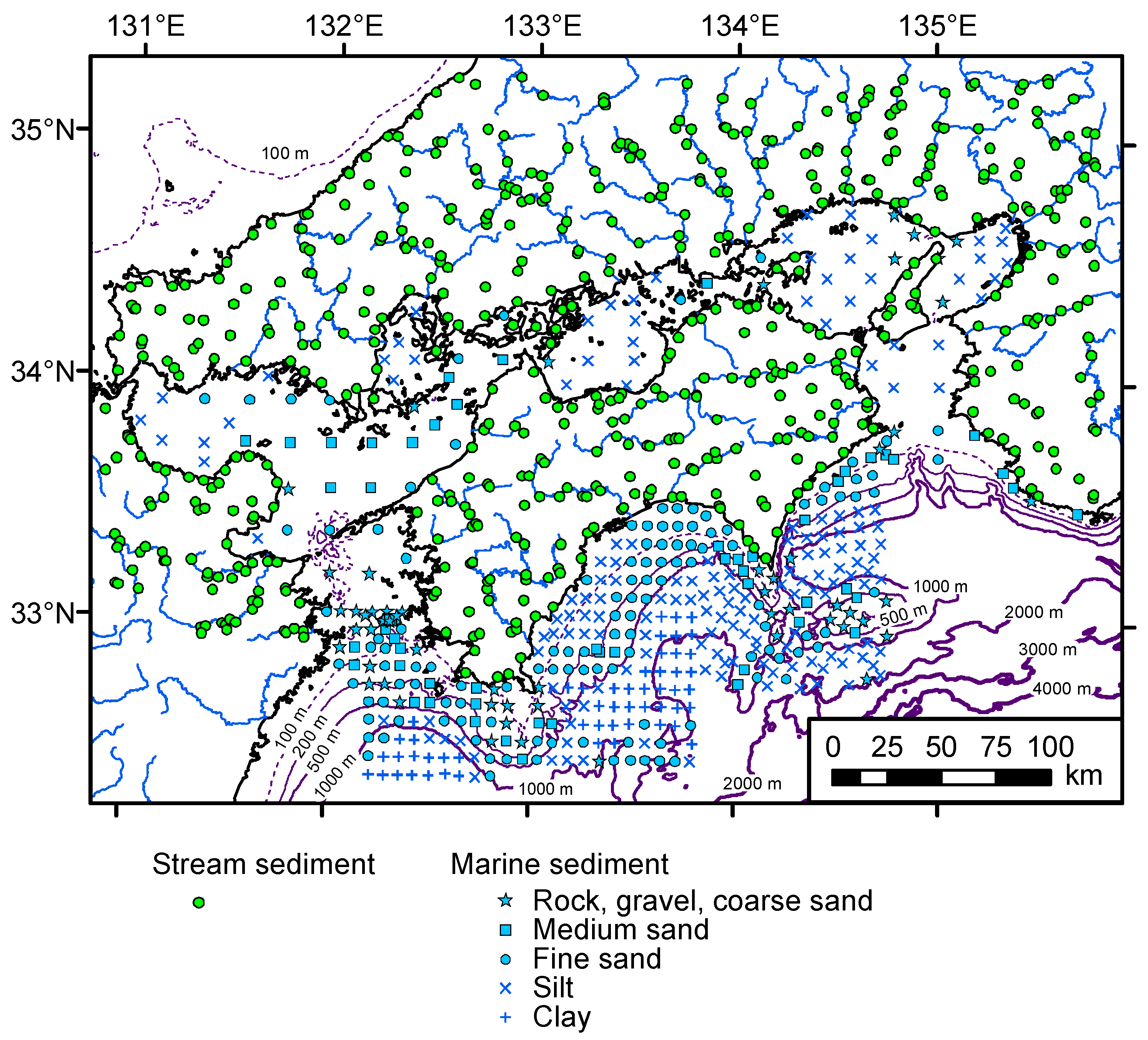
3.1. Samples, Sampling Methods, and Processing

Terrestrial and marine sampling locations are presented in Figure 3. A total of 554 stream samples were collected from the study area for a regional geochemical mapping project during 1999–2004 [22]. In addition, for the current study, 22 stream sediments were collected in 2008 from small islands, including Awaji Island in the Seto Inland Sea. Sediment sample were air-dried and sieved using a 180 μm (83-mesh) screen. Magnetic minerals were removed from the sieved samples using a magnet, to minimize the effect of magnetic mineral accumulation [22,23].
A total of 366 marine samples were collected from the Pacific Ocean during cruises GH82-1 and GH83-2, in 1982 and 1983, respectively [24,25,26]. In addition, 97 samples were collected from the Seto Inland Sea and around the Kii Peninsula in 2005. The total 463 samples were collected using a K-grab sampler, and the uppermost 3 cm of each sediment sample was separated, air-dried, ground with an agate mortar and pestle, and retained for chemical analysis. Some samples were composed mainly of rock fragments and gravels, in which case, the sandy infilling materials were collected. The particle sizes of 223 marine sediments were determined, based on the median particle diameter of the surface sediments, and were classified as: coarse sediments, comprising lithic fragments, gravels, and coarse sand; medium sand; fine sand; silt; and clay (Figure 3). The median particle diameter was not measured for the remaining 240 samples, so their classification is based solely on a visual inspection of texture.
Figure 3 shows that silty sediments occur in Suo-Nada, Hiuchi-Nada, Bingo-Nada, and Harima-Nada, as well as basins affected by small periodic current flows or eddies [10]. These localities are also associated with high turbidity [12,27]. Coarse sands were collected from Aki-Nada and Bisan-Seto-Nada, and in northeastern Iyo-Nada. Rocks, gravels, and coarse sands occur in the Bungo Channel. In contrast, the Kii Channel is dominated by silty sediments, despite the presence of high velocity periodic currents similar to those in the Bungo Channel. This is likely due to the greater terrestrial sediment supply to the Kii Channel (18%) compared with the Bungo Channel (1%) (Table 1). On the Pacific side, silty sediments are widely distributed obliquely across the depth contour in the western part of Tosa Bay. Fine sands are found: (1) near to river mouths; (2) at water depths of 100–500 m on the shelf and slope off Tosa Bay; and (3) around Ashizuri Knoll and Muroto Knoll where the water depth is 500–1600 m. Silty and clayey sediments are found in Tosa Basin, Hyuga Basin, and Muroto Trough, where the water depth exceeds 1000 m, and rock, gravels, and coarse sands were sampled from the topographic highs of Ashizuri Spar, Muroto Spar, and Tosa-Bae.

3.2. Geochemical and Spatial Analyses

The geochemical analytical method is detailed by Imai [28]. Each 0.2 g sample was digested using HF, HNO3, and HClO4 solutions at 120 °C for 2 h. The degraded solution was evaporated to dryness at 200 °C, before the residue was dissolved in 100 mL of 0.35 M HNO3 solution. Concentrations of Na2O, MgO, Al2O3, P2O5, K2O, CaO, MnO, total (T-) Fe2O3, V, Sr, and Ba were determined using ICP atomic emission spectrometry, while contents of Li, Be, Sc, Cr, Co, Ni, Cu, Zn, Ga, Rb, Nb, Y, Mo, Cd, Sn, Sb, Cs, lanthanides (Ln: La–Lu), Ta, Tl, Pb, Bi, Th, and U were measured using ICP mass spectrometry. Analyses of As in all samples and Hg in stream sediment samples were subcontracted to ALS Chemex in Vancouver, B.C. Levels of Hg in marine sediments were determined using an atomic absorption spectrometer that measured the quantity of Hg vapor generated by direct thermal decomposition. Table 2 presents a summary of the analytical results obtained from the marine and stream sediments. The Na2O component of marine sediments should be used only as a guide, since these marine sediments were not desalinated.
The spatial distributions of elemental concentrations in both the terrestrial and marine environments were plotted using geographic information system software (ArcGIS 10.3; Environmental Systems Research Institute (ESRI) Japan Corporation, Tokyo, Japan) after Ohta et al. [29]. Different classes of elemental concentrations are applied to the terrestrial and marine environments, because the chemical and mineralogical compositions of sediments differ according to particle size see the details in [7,8]. This simply improves geovisualization of the geochemical maps. If the same classification is applied to the geochemical maps of both terrestrial and marine environments, the regional geochemical differences (as depicted by color variation) of most of the elements in the land or the sea will be obscured [7,8]. For example, for CaO and Sr, which show higher concentrations in the marine sediments (Table 2), their geochemical differences in the terrestrial areas would be obscured in resulting maps using the same classification, as shown in the Legend. Percentile ranges are used for the selection of elemental concentration intervals in the geochemical maps: 0 ≤ x ≤ 5, 5 < x ≤ 10, 10 < x ≤ 25, 25 < x ≤ 50, 50 < x ≤ 75, 75 < x ≤ 90, 90 < x ≤ 95, and 95 < x ≤ 100%, where x represents the elemental concentration [30]. This class selection is advantageous in that the same range of percentiles (e.g., 90%–95%) implies the same statistical weight, even at different numerical scales [7,8,30]. Subsequent statistical analysis of geochemical data is performed using EXCEL TOUKEI 7.0 (ESUMI Co. Ltd., Tokyo, Japan).

4. Results

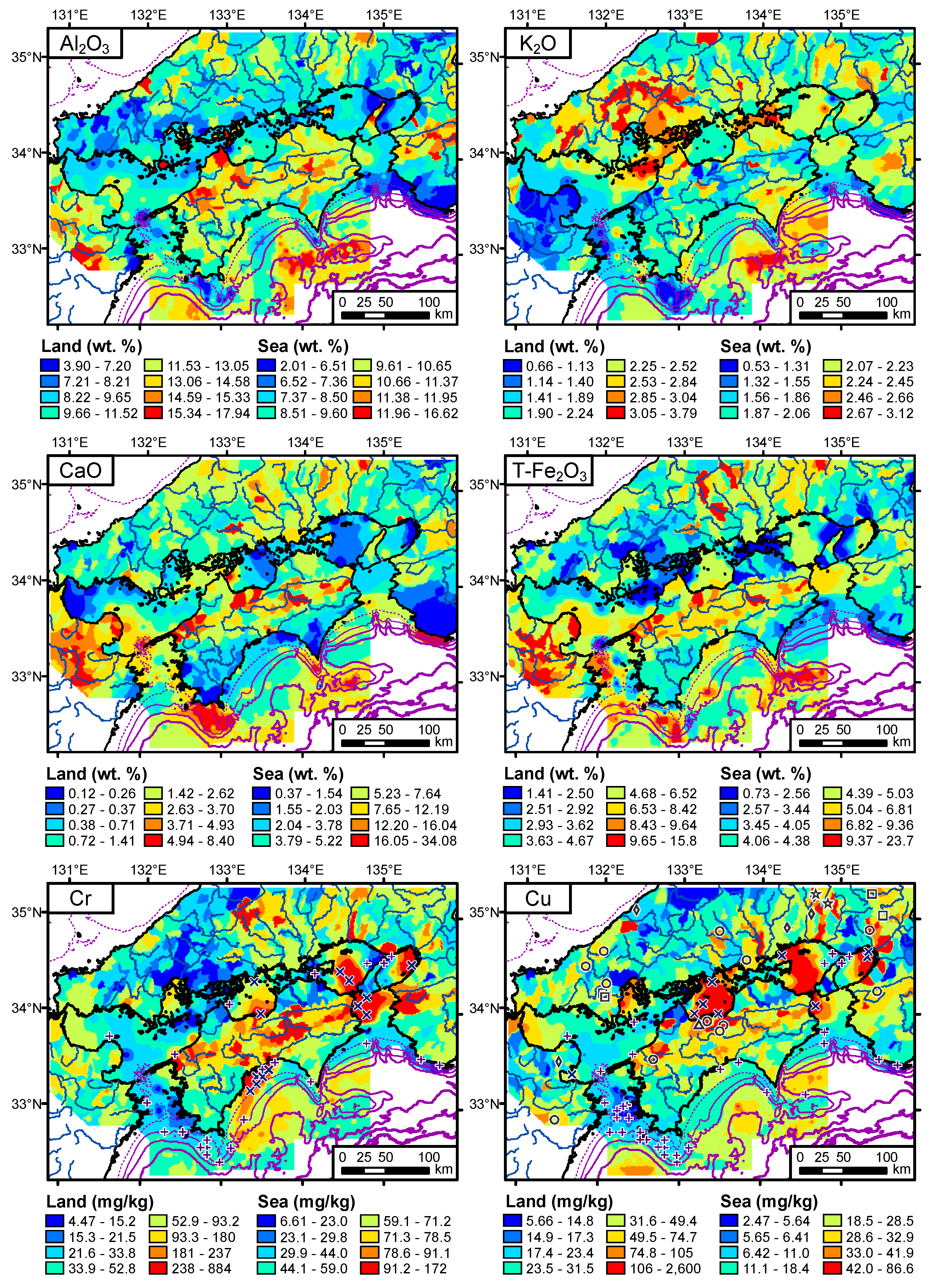
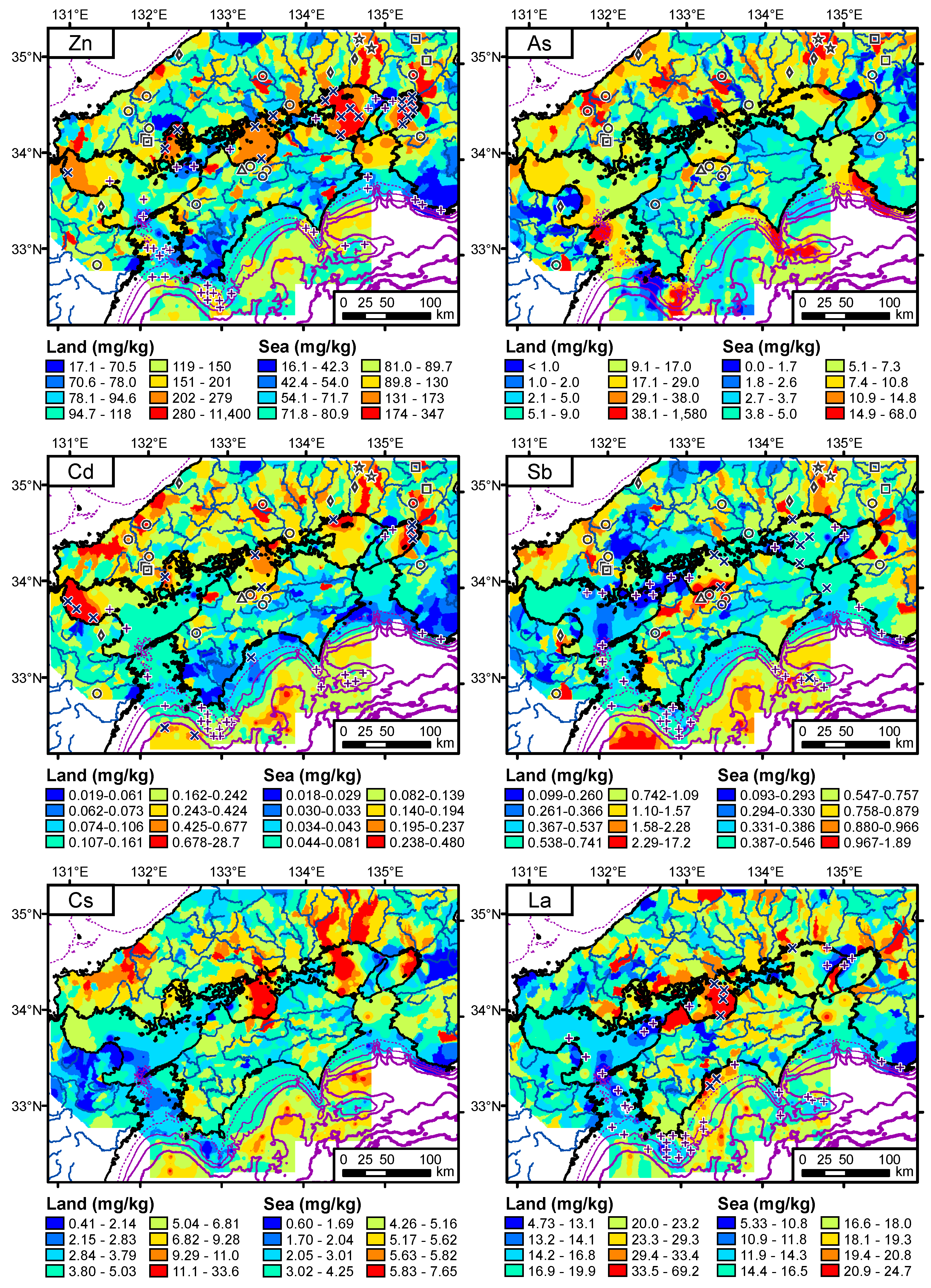
4.1. Spatial Distribution of Terrestrial Elemental Concentrations

Figure 4 shows the terrestrial and marine geochemical maps for 12 elements. Mikoshiba et al. [23] and Ohta et al. [31,32] have examined the factors controlling spatial distribution patterns of terrestrial elemental concentrations. Be, Na2O, K2O, Rb, Y, Nb, Ba, Ln, Ta, Th, and U are abundant in the Chugoku region and in the northern part of Shikoku Island where predominantly granitic and felsic volcanic rocks outcrop. Stream sediments derived from granitic rocks are enriched in Li, Be, Na2O, K2O, Rb, Y, Nb, Ln, Ta, Th, and U. Felsic volcanic rocks also elevate the K2O, Rb, and Ba contents of stream sediments. Li and Cs are abundant in muddy sedimentary rocks and the mélange matrix of accretionary complexes in northern Kinki. In contrast, the sandstone-dominated sedimentary rocks of accretionary complexes in the southern part of Shikoku Island and the Kii Peninsula contain fewer elements. Mafic volcanic rocks associated with debris flows and pyroclastic rocks around Aso volcano, and metamorphic rocks, dominantly greenschist, on Shikoku Island and the Kii Peninsula, elevate MgO, Al2O3, P2O5, CaO, Sc, V, TiO2, MnO, T-Fe2O3, Cr, Co, Ni, and Cu concentrations in the stream sediments. Additionally, extreme enrichments of MgO, Cr, Co, and Ni are caused by the presence of mafic-ultramafic rocks associated with accretionary complexes. Finally, elevated concentrations of P2O5, Cu, Zn, Mo, Cd, Sn, Sb, Hg, Pb and Bi are found in Osaka Plain, which is polluted by anthropogenic activity [32].
Therefore, lithology is considered to be the main factor affecting the concentrations of elements in stream sediments. For reference, the median elemental concentrations of stream sediments according to their representative rock type, which outcrops over more than half of the drainage basin, are summarized in Appendix B. It should be noted that Cu, Zn, As, Mo, Cd, Sn, Sb, Hg, Pb, and Bi are extremely enriched near to known metalliferous deposits, however, the effects of these mineral deposits on the geochemical maps are restricted to limited areas.

4.2. Spatial Distribution of Elemental Concentrations in Coastal Sea Sediments

Within the Seto Inland Sea, high levels of K2O, Rb, Ba, and Tl are found in the coarse sands of Aki-Nada and Bisan-Seto-Nada, and in northeastern Iyo-Nada (Figure 4). Coarse sediments with rock fragments, gravels, and coarse sands in western Iyo-Nada and the Bungo Channel are enriched in MgO, P2O5, CaO, TiO2, MnO, Fe2O3, Sc, V, Co, Zn, and Sr. In contrast, the sandy sediments in eastern Iyo-Nada and the Bungo Channel are depleted in almost all of the measured elements, except CaO and Sr. Silt and clay in Hiuchi-Nada, Harima-Nada, and the Kii Channel are abundant in Li, Be, MgO, P2O5, 3d transition metals, Ga, Y, Nb, Sn, Cs, Ln, Ta, Hg, Pb, Bi, and Th. Suo-Nada is enriched in Li, Zn, Ga, Sn, Mo, Cd, Ta, Pb, Bi, and U. Concentrations of P2O5, Cr, Ni, Cu, Zn, Mo, Cd, Sn, Hg, Pb, and Bi are especially elevated in the silt of Osaka Bay. Finally, MnO and Tl are abundant in all sediments within the Seto Inland Sea, irrespective of particle size.
On the Pacific Ocean side, coarse sediments with rock fragments, gravels, and coarse sands distributed around the topographic highs of Ashizuri Spar, Muroto Spar, Tosa-Bae, and the Muroto Sea Knoll are abundant in MgO, CaO, Al2O3, P2O5, TiO2, MnO, T-Fe2O3, Sc, V, Co, As, Sr, Mo, Sb, and U. Sediments abundant in TiO2, Cr, Co, Ni, Nb, light REEs (lanthanides from La to Sm), and Ta, occur in Tosa Bay. The silty and clayey sediments of Tosa Basin, Hyuga Basin, and the Muroto trough are enriched in Li, Cu, Nb, Cd, Sb, Cs, Hg, and U. Fine sands collected from the Ashizuri and Muroto Sea Knolls are richer in P2O5, CaO, Sc, TiO2, V, MnO, Fe2O3, Co, Cu, As, Sr, Mo, Cd, Sb, Cs, heavy REEs (Y and lanthanides from Gd to Lu), and Bi than the fine sands distributed across the continental shelf.

5. Discussion

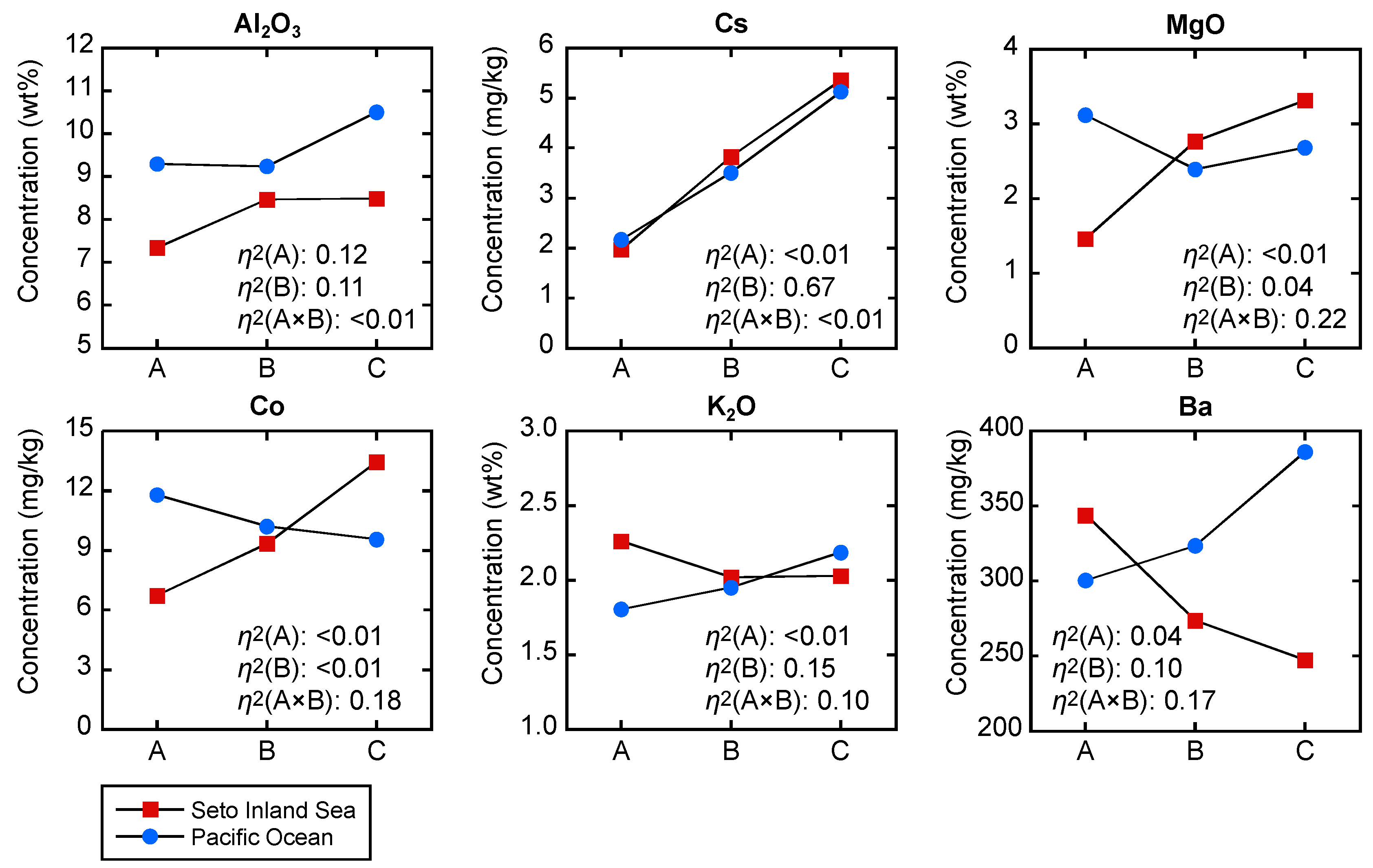
5.1. Analysis of Variance (ANOVA) to Reveal the Effects of Particle Size and Regional Difference

Coastal sea sediments typically originate from their adjacent terrestrial materials. Therefore, the geochemical features of terrestrial lithology are fundamentally reflected in those of nearby marine sediments. This phenomenon is referred to herein as “regional difference”. Additionally, elemental concentrations in marine sediments are known to vary with particle size, in a phenomenon referred to herein as the “particle size effect”. This variation is caused simply by the dilution effects of quartz and biogenic calcareous materials, which are abundant in coarse grains but less abundant in fine grains. Thus, we apply a two-way analysis of variance (ANOVA) to determine the factor that most significantly controls the chemical compositions of marine sediments: regional differences or the particle size effect [8]. The procedure is detailed by [8] (Appendix C).
The marine samples are grouped into those from the Seto Inland Sea region, including the Kii and Bungo Channels, and those from the Pacific Ocean region. They are further classified into: coarse sediments, including rock fragments, gravels, coarse sands, and medium sands; fine sands; and silt-clay. We assume that the coarse sediments, fine sands, and silt-clay are moved by water power over short, middle, and long distances, respectively. Median elemental concentrations of marine sediments are calculated for each region and particle size (Table 3). Table 3 also presents the median concentrations of stream sediments from two regions, for reference. In this regard, 96 stream sediment samples were collected from rivers that flow directly into the Sea of Japan, and so these samples are excluded from Table 3.
Table 4 presents the results of a two-way ANOVA: the variance ratios (F), probabilities (p), and effect size (η2) due to regional difference (factor A), particle size (factor B), and the interaction effect (factor A × B). When the estimated probability is lower than 0.01, we conclude that the factor makes a significant difference to the chemical compositions, and in fact, each factor was statistically significant (p < 0.01) in most cases (Table 4). This is because a statistical test with a large amount of input data, such as n = 463 in this study, is highly sensitive to very small differences. Therefore, we calculate η2 to form a plausible estimation of p value irrespective of sample number [33,34]. The η2 is an easy-to-understand metric that is calculated as the ratio of the sum of squares (SS) for each factor and the total SS. Magnitudes of η2 < 0.01, 0.01 ≤ η2 < 0.06, 0.06 ≤ η2 < 0.14, and η2 ≥ 0.14 can be considered to represent no effect, a small effect, an intermediate effect, and a large effect, respectively [33,34]. In this study, we conclude that each factor with η2 ≥ 0.06 has a significant effect on the elemental concentrations of the sediments. Furthermore, this indicator can be used to decide the most dominant factor, on the basis of the highest η2 score [33].
Results of the ANOVA suggest that particle size is the dominant influencing factor for many elements in the sediments (Table 4). The regional difference effect is more significant than the particle size effect only for Al2O3, CaO, MnO, Sc, V, Mo, and Pb. This suggests that consideration of the particle size effect must be made in order to fully understand the influence of terrestrial materials on coastal sea sediments. However, it should be noted that the interaction effect is more influential than either of the two main factors alone for MgO, P2O5, Fe2O3, Sc, Co, Rb, Ba, and Eu, and is significant for 14 elements, including K2O and TiO2. This interaction effect refers to the effect of one factor on the other factor, such that the two main factors synergistically affect the data e.g., [35]. To visualize the interaction effect, variations in the median values of Al2O3, MgO, K2O, Co, Cs, and Ba are presented in Figure 5. When the interaction effect is insignificant, the median values vary approximately in parallel between the Seto Inland Sea and the Pacific Ocean, irrespective of particle size (Al2O3 and Cs in Figure 5). In the cases of large η2 values for the interaction effect, such as for MgO and Co, the elemental concentrations in the Pacific Ocean sediments decrease with decreasing particle size, but increase in the sediments of the Seto Inland Sea with decreasing particle size. Variations in the K2O and Ba concentrations with particle size are exactly opposite to those of MgO and Co, and still indicate a significant contribution of the interaction effect. These results suggest that regional difference and particle size effects are not independent for many elements. Therefore, we need to evaluate the geochemical similarities and differences among groups subdivided by region and particle size.

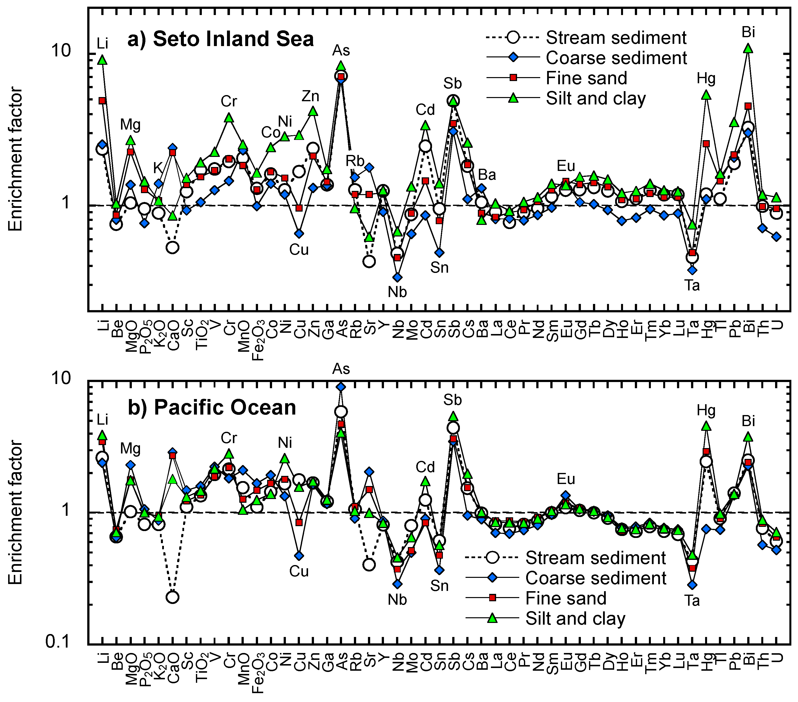
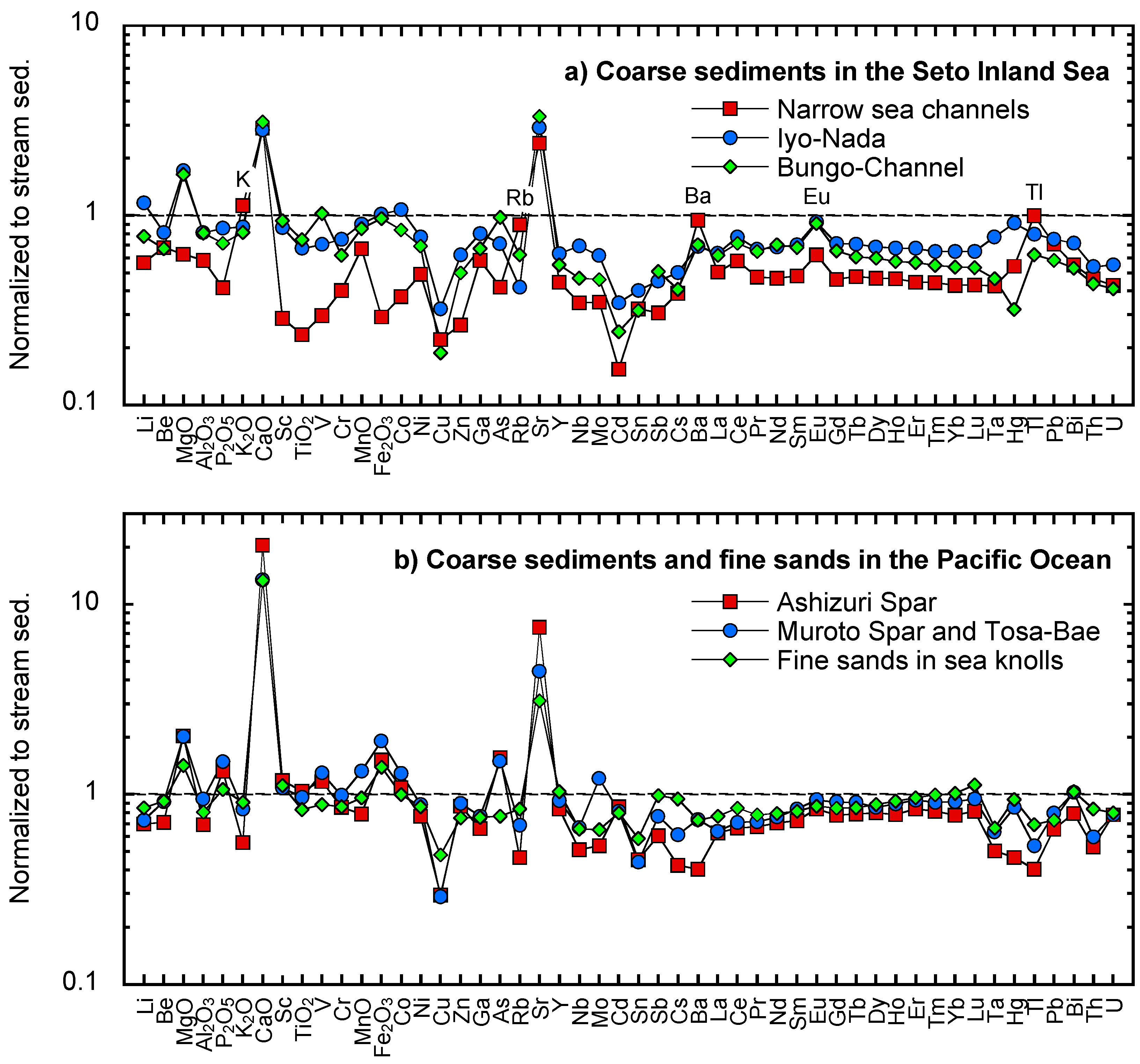
5.2. Comparison of Elemental Abundances in Coastal Sea and Stream Sediments between the Seto Inland Sea and the Pacific Ocean

The chemical and mineralogical compositions of marine sediments differ from those of stream sediments [7,8]. Furthermore, the range in concentration completely differs for each element: major and minor elements in wt % oxide amounts, and trace elements in mg/kg or μg/kg amounts. Therefore, to eliminate the effect of scale and units, the data have to be normalized to elucidate differences amongst the elements or the samples. Thus, in this study, enrichment factors (EF) of the marine and stream sediments compared with the upper continental crust (UCC) [36] are employed to allow direct comparison (Figure 6). The EF is calculated as follows:
EF = ([C]sample/[Al2O3]sample)/([C]UCC/[Al2O3]UCC),
where [C] and [Al2O3] are the concentrations of a given element and Al2O3, respectively. Al2O3 is a major element group, and a dominant constituent of many minerals such as plagioclase. Therefore by using it to normalize the EFs, we can effectively remove the effects of quartz, calcareous materials, and organic matter [8]. The systematically high EFs of Li, As, Sb, Hg, and Bi, and low EFs of Nb, Sn, and Ta for all samples, as well as CaO and Sr in stream sediments, are fundamental geochemical signatures of upper crust materials in an island arc setting [37] (Figure 6a,b). The high abundance ratios of CaO and Sr in marine sediments indicate the presence of biogenic calcareous materials, such as shell fragments and foraminifera tests. In the Seto Inland Sea, the UCC normalized patterns of fine sands are similar to those of stream sediments (Figure 6a). Abundance ratios of most elements in marine sediments decrease with increasing grain size. CaO, K2O, Rb, Sr, and Ba are especially dominant in coarse sediments, whereas silt and clay have higher abundance ratios for Li, Cr, Co, Ni, Zn, Mo, Cd, Cs, Hg, Pb, and Bi. In the Pacific Ocean, the UCC normalized patterns of fine sands and silt-clay samples are most similar to those of stream sediments (Figure 6b). The variations in EF of most elements with particle size of the marine sediments in the Pacific Ocean are likely smaller than those for samples in the Seto Inland Sea, except for MnO, As, Ce, Eu, and Tl. Coarse sediments have relatively high abundance ratios for MnO, Fe2O3, Co, and As, and low abundance ratios for Li, Cu, Nb, Sn, Cs, light REEs, Ta, Hg, Tl, Th, and U. The silty and clayey sediments are particularly enriched in Cr, Ni, Cu, Cd, Sb, Hg, and Bi.

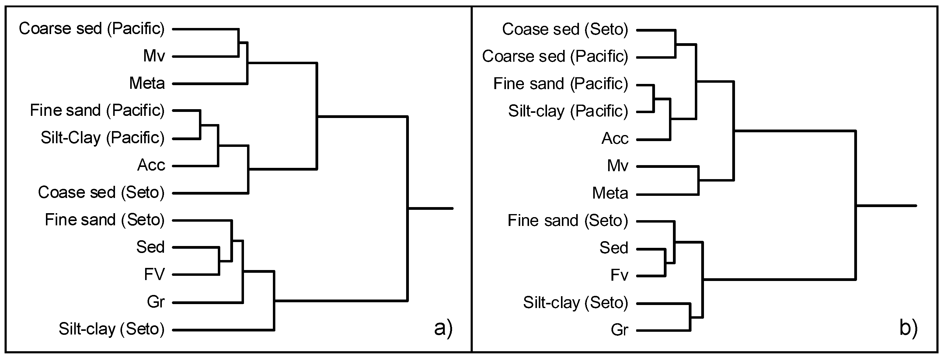
5.3. Discrimination of Coastal Sea Sediments Using Cluster Analysis

Coarse sediments have UCC normalized patterns that notably differ from those of terrestrial materials (Figure 6a,b), which implies that they have different origins to the modern terrestrial materials or are supplied by a particular lithology. Thus, we refine the identification of probable source materials for marine sediments using cluster analysis. The classification of marine sediment samples is as presented in Table 3. Stream sediments grouped according to the seven rock types summarized in Table B1 are used for comparison. The distance between data points was calculated as a Euclidian distance, requiring the geochemical data from marine and stream sediments to be standardized or transformed appropriately. This is because the compositional data constitute “closed” data that sum to a constant [38,39]. To mitigate biased analysis arising from data closure, there is a requirement for data transformation to yield data with normal distributions suitable for parametric statistical analysis. Additive log-ratio, the centered log-ratio, and the isometric log-ratio transformation of compositional data have been proposed [38,39]. We used a log transformation of the EF data to generate logarithmic EFs for each sample, which were used as the input data for cluster analysis. The logarithmic EF corresponds to the additive log-ratio transformation of the compositional data [38,39]:
log EF = alr(C)sample − alr(C)UCC,
where alr(C) stands for additive log-ratio transformation (log {[C]/[Al2O3]}). We have confirmed that the EF is effective in eliminating the effect of scale and units, and in removing the dilution effect, although Al2O3 concentration is empirically used for denominator in Equation (1). The logarithmic EF also incorporates data normality and is thus amenable to multivariate parametric tests such as cluster analysis.
Figure 7 presents dendrograms that show the distances between two points. The distances between clusters were obtained by Ward’s method [40]. We calculated two kinds of dendrograms using different combinations of elements. Figure 7a uses a dataset that excludes sea salt (Na2O), biogenic carbonate materials (CaO and Sr), and heavy metals related to mining and anthropogenic activities (As, Mo, Cd, Sn, Sb, Hg, Pb, and Bi), which do not reflect the geochemistry of the parent lithology. Figure 7b uses the EFs of immobile elements (Sc, TiO2, Cr, Nb, Ta, Y, Ln, and Th), which are not strongly influenced by weathering processes. The obtained dendrograms are mutually similar (Figure 7a,b). Coarse sediments from the Pacific Ocean plot in the same group as stream sediments derived from mafic volcanic and metamorphic rocks in Figure 7a. However, Figure 7b shows that all marine sediments in the Pacific Ocean cluster together with coarse sediments from Seto Inland Sea and accretionary complexes. Fine sand and silt-clay in the Pacific Ocean and coarse sands in the Seto Inland Sea are always grouped together with stream sediments derived from sedimentary rocks of accretionary complexes. These results for fine sands and silt-clay are reasonable, because such sedimentary rocks outcrop extensively across the southern part of Shikoku Island (Figure 2), which supplies the highest sediment yield to the Pacific Ocean (Table 1). In contrast, the fine sands and silt-clay in the Seto Inland Sea plot with those stream sediments derived from granitic and felsic volcanic rocks. This result is also expected, due to the extensive outcropping of these rock types across the Chugoku region, which supplies the highest sediment yield to the Seto Inland Sea (Table 1).

5.4. Discrepancies in the Geochemistry of Coarse Marine Sediments and Stream Sediments

5.4.1. Fractionation of Mineralogical Compositions in Coarse Sediments by a Strong Tidal Current

Cluster analysis suggests that the coarse sediments in the Seto Inland Sea are related to stream sediments sourced from sedimentary rocks of accretionary complexes. However, granitic and felsic volcanic rocks are geographically more suitable sources for the coarse sediments, in analogy with the fine sands. To reveal their geochemical features in more detail, Figure 8a shows the abundance patterns of elements in coarse sediments collected from the narrow sea channels (Aki-Nada, Bisan-Seto-Nada and around Awaji Island), Iyo-Nada, and Bungo Channel, normalized to the stream sediments in the Seto Inland Sea region.
Coarse sands in the narrow sea channels are particularly rich in K2O, CaO, Rb, Sr, Ba, and Tl, and have a distinctive positive Eu anomaly, but are extremely depleted in many elements, such as Sc and TiO2 (Figure 8a). These features are indicative of the selective accumulation of biogenic calcareous materials, quartz, and alkali-feldspars. Quartz and alkali-feldspar are abundant in granitic and felsic volcanic rocks, and are highly resistant to weathering processes, so are preserved as coarse particles e.g., [41]. In contrast, the coarse sediments in Iyo-Nada and the Bungo Channel are relatively abundant in MgO, P2O5, CaO, Sc, TiO2, V, Fe2O3, Co, and Zn in addition to the elements mentioned above (Figure 8a). These additional elements are found abundantly in mafic minerals such as biotite, hornblende, and pyroxene, as well as accessary minerals such as magnetite and ilmenite. We therefore assume that the fine particles of mafic and accessary minerals are swept away from the narrow sea channels by a strong tidal current, but this does not occur in Iyo-Nada and the Bungo Channel. In contrast, the coarse grains in all areas are rarely moved over any long distances by water power.

5.4.2. Denudation of the Basement Rocks of the Topographic Highs

Cluster analysis provides different results for coarse sediments from the Pacific Ocean (compare Figure 7a,b). This is because only three elements (Sc, TiO2, and Cr) abundant in sediments derived from mafic volcanic rocks and metamorphic rocks (dominantly greenschist) are used in the cluster analysis of the immobile element dataset (Figure 7b). Thus, cluster analysis using immobile elements may be poorly sensitive to such rock types. Consequently, we conclude that Figure 7a would provide a more plausible result: mafic volcanic and metamorphic rocks are the probable sources of coarse sediments in the Pacific Ocean. However, these rock types are located relatively distantly from the coarse sediment deposition sites (Figure 2). The high EFs of MnO, Fe2O3, Co, and As in coarse sediments from the Pacific Ocean (Figure 6b) can be explained by Fe hydroxide and Mn dioxide coatings on coarse particles and gravel (for example, T-Fe2O3 and As; Figure 4). In this regard, relict quartz particles coated with Fe hydroxides are found in the Bungo Channel [26]. However, this explanation does not fully account for the enrichment of MgO, P2O5, Sc, TiO2, and V. According to Okamura [19], the topographic highs in this region are formed from basement rocks of Miocene–Pliocene siltstone. These highs typically have a low sedimentation rate and are located in a region of erosion, due to the strong bottom flow associated with the Kuroshio Current [24]. The spar and knoll sediments are therefore assumed to have formed by denudation of the basement rocks (siltstone), which have a different lithology to the southern part of Shikoku Island. Therefore, we assume that basement rocks of siltstone might be influenced by mafic volcanic activity at Miocene-Pliocene age. Figure 8b shows the abundance of elements in coarse or gravelly spar sediments and knoll sediments (mainly fine sands), normalized to the stream sediments in the Pacific Ocean region. Despite the fact that Ashizuri Spar is more than 100 km away from Muroto Spar and Tosa-Bae, the abundance patterns of the coarse spar sediments are very similar. Furthermore, the fine sands collected around Ashizuri Knoll and Muroto Knoll have similar abundance patterns to those of the coarse spar sediments. As such, the unexpected cluster analysis result for coarse sediments in this region can be explained by mineral segregation under a strong tidal current unique to the Seto Inland Sea, and by a denudation of old basement rocks (Miocene–Pliocene siltstone) in the Pacific Ocean.

5.5. The Transfer of Silty and Clayey Sediments Influenced by Periodic Currents, Tidal Currents, and a Water Mass Boundary

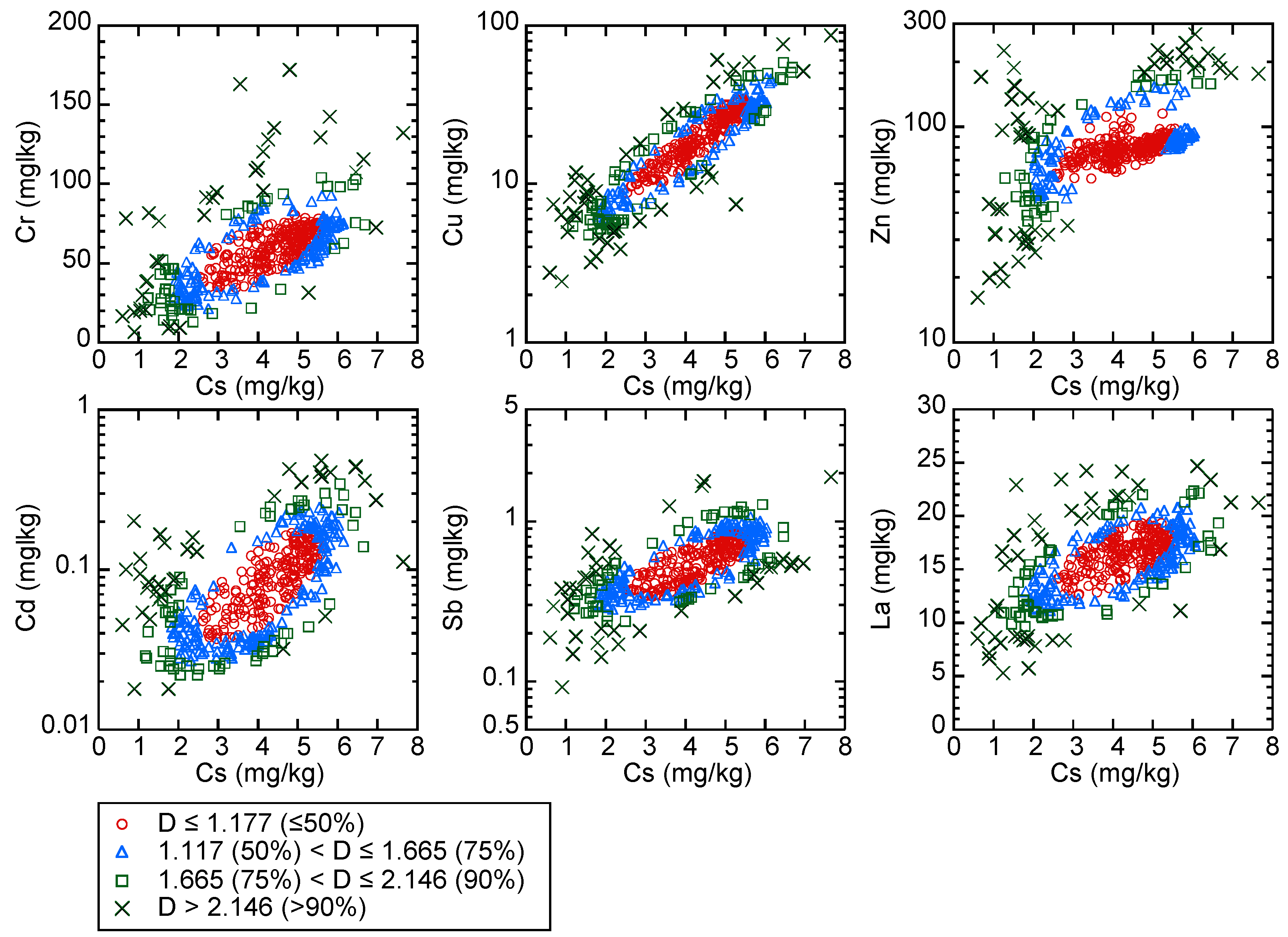
5.5.1. Mahalanobis’ Generalized Distances for Finding Outliers

Silty and clayey sediments supplied from rivers take a long time to reach the sea floor. Therefore, their spatial distribution is a result of conveyance and dispersion by coastal sea currents. Ohta and Imai [7] and Ohta et al. [8] simply focused on the spatial distribution patterns of high Cr and Ni concentrations in silty sediments, which are indicative of transport of fine particles from land to sea or marine environments. Their spatial distribution can be easily discriminated because they are extremely enriched in silty marine sediments derived from ultramafic rocks in the adjacent terrestrial area. Ohta et al. [42] tried to visualize the particle transfer process using the spatial distribution patterns of the other elements. However, many elements are enriched in finer sediments due to the particle size effect, and so in order to highlight the particle transfer process, it is useful to detect outliers using the relationships between elemental concentrations and median diameter or mud content [42].
Unfortunately, in this study, data of median diameter or mud content are available for only half of the samples. ANOVA analyses suggest that Cs, Hg and Th concentrations in marine sediments are determined only by particle size and are not sensitive at all to either regional differences or interaction effects (η2 < 0.01) (Table 4). The particle size effect of Cs has the largest η2 score of the three elements, suggesting that the particle size effect has the maximum effect on Cs concentrations. Although concentrations of 13 elements, including Cr, Cu, and La, in marine sediments are also controlled dominantly by particle size effects, they are further influenced weakly by regional difference effects and interaction effects (0.01 ≤ η2 < 0.06) (Table 4). In addition, Hg, Cu, and Cd concentrations in marine sediments might be influenced by metalliferous deposits and anthropogenic activity in the adjacent terrestrial area. For these reasons, we conveniently use Cs concentration as a proxy for the median diameter or mud content.
Figure 9 shows the relationships between Cr, Cu, Zn, Cd, Sb, and La concentrations and that of Cs. The concentrations of all six elements correlate positively and linearly with Cs, and it can be assumed that those samples plotting outside the linear trends are subject to influencing factors in addition to the particle size effect. Ohta et al. [42] detected outliers from a scatter diagram according to their best judgment. In this study, the outliers appearing in the scatter diagram are objectively obtained using Mahalanobis’ generalized distance (D) [43]. This method presupposes that the data follow a normal distribution similar to ANOVA. Thus, the data transformation is given in Table C1. The obtained D values gradually increase from the inner part of the data cluster to the outer part, giving an onion-like structure (Figure 9). D values of D ≤ 1.117, D ≤ 1.665, and D ≤ 2.146 indicate that 50%, 75%, and 90% of the total data points are included, respectively, and data points are defined as an outlier herein if D > 2.146, which includes the upper and lower 5% of multivariate outliers. The outliers were determined from all datasets, so silt and clay classified as outliers are expressed as cross symbols; while coarse sediments and fine sands classified as outliers are expressed as plus symbols in Figure 4.

5.5.2. Transport of Elements in Silt Derived from the Parent Lithology

Figure 4 shows that the locations of the outliers calculated for Cr (cross symbols) correspond with a NNW-SSE distribution of silty-clayey sediments with high Cr concentrations in the Kii Channel. This distribution of Cr outliers indicates that silty particles that originated from ultramafic rocks are supplied through the Yoshino, Naka, and Kino Rivers to the Kii Channel, and are then widely dispersed by a periodic current, as Ohta and Imai [7] noted. Hiuchi-Nada also contains abundant silty sediments, however the distribution of outliers (corresponding to high concentration areas) for MgO, Cr, Co, and Ni is restricted to the vicinity of Shikoku Island (shown by Cr in Figure 4). This can be explained by the fact that the terrestrial sediment discharge yield to Hiuchi-Nada is minimal compared to the output of the Yoshino River, Naka River and Kino River systems (Table 1).
Y, Nb, Ln, Ta and Th are also enriched in the silty sediments of Hiuchi-Nada, especially in the eastern part (La in Figure 4). The differing distributions of La and Cr outliers suggest that Y, Nb, Ln, Ta and Th have a different origin from MgO, Cr, Co, and Ni. Minakawa et al. [44] reported that rare earth minerals, including allanite and monazite, occur within pegmatite veins of the Ryoke granitic rocks, which outcrop in northwest Shikoku Island, on the small islands in Aki-Nada and Bisan-Seto-Nada, and are partly exposed on the seafloor [12]. Yanagi [10] suggested that fine particles transported by periodic currents accumulate in eastern Hiuchi-Nada where the amplitude of the tidal current is small and a counterclockwise circulation occurs. Consequently, we assume that silt enriched in rare earth minerals has been swept toward the eastern side of Hiuchi-Nada by periodic currents and accumulated there over a long period of time.
In Tosa Bay, tongue-shaped distribution patterns of high MgO, Cr, Co, Ni, Nb, Y, Ln, Ta, and Th concentrations and their outliers are apparent (shown by Cr and La in Figure 4). MgO, Cr, Co, and Ni originated from ultramafic rocks, while the other elements are derived from greenstones wedged between the Sambagawa metamorphic rocks and accretionary complexes e.g., [45]. Ikehara [25] and Hoshino [46] reported that silty and clayey sediments are selectively deposited at the boundary between coastal waters with low salinity (due to River input) and the outer sea with higher salinity. This is supported by the fact that the water discharges from the Niyodo and Shimanto Rivers into Tosa Bay are among the largest in the region (Table A1). Thus, on the basis of this evidence, sedimentation at the boundary between water masses can explain this distinctive distribution [7]. In addition, the countercurrent of the Kuroshio Current, which flows in a counterclockwise direction on the continental shelf (Figure 1b), may also contribute to the transport of fine particles enriched in the elements mentioned above [21].

5.5.3. Transfer of Materials Related to Mineral Deposits and Anthropogenic Activity

A number of silty sediment samples in Hiuchi-Nada are abundant in Cu (40.6–86.6 mg/kg) and are classified as outliers (Figure 4); these reflect the mining activity at the nearby Besshi Cu mines over the past 240 years [47]. Similarly, the outlier observed within the Kii Channel sediments is related to activity at the Cu mine in the watershed of the Yoshino River. In addition, one outlier for Sb (1.89 mg/kg) is found near to the shore in southern Hiuchi-Nada. This enrichment of Sb suggests contamination from the Ichinose Sb mine, which is located close to the Besshi mine.
Osaka Bay is adjacent to Osaka City, which is the second largest city in Japan and has a long history of industrial development. Ohta et al. [32] found that Cu, Zn, Cd, Sn, Sb, Hg, and Pb are significantly enriched in stream sediments collected from the urban areas of Osaka Plain. Similarly, the silty sediments in Osaka Bay are highly enriched in Cr, Cu, Zn, As, Mo, Cd, Sn, Hg, Pb, and Bi (as shown by Cr, Cu, Zn, and As in Figure 4). Samples with the top 1% of concentrations for these elements, which are mostly classified as outliers, are found in Osaka Bay, and the area of high concentrations near the mouth of the Yodo and Yamato Rivers is clearly due to the discharge of contaminated sediments. Hoshika and Shiozawa [27], Hoshika et al. [48], and Manabe [49] reported the same results, showing large accumulations of Cr, Cu, Zn, Cd, Pb, and Hg in Osaka Bay.
A number of outliers of Cu, Zn, Cd, Sn, Pb, and Bi are also found in Harima-Nada, Hiroshima Bay and Suo-Nada (shown by Cu, Zn, and Cd in Figure 4). Their enrichment may be a result of the nearby metalliferous deposits and contamination by the coastal industrial zones [49,50]. In particular, Ikuno mine is considered a possible source for the elements abundant in Harima-Nada because it is one of the largest hydrothermal-type polymetallic mines, bearing Cu, Zn, As, Cd, Sb, Sn, Pb, and Bi [31] (Figure 2). However, the spatial distributions of the outliers are different for each enriched element. A likely explanation for this is that the rivers flowing through the mineralized zones are small and have much smaller sediment discharges. Alternatively, the elements may have been released in the water during the oxidation of sulfide ores, and have subsequently absorbed into the surface sediment of the coastal seas [51].

5.5.4. Geochemical Features of Silt and Clay in the Deep Sea Basins of the Pacific Ocean

Silt and clay deposited in deep Pacific basins are typically enriched in MnO, V, Ni, Co, Mo, Sb, Pb, and Bi, as a result of early diagenetic processes in an oxic environment [7,42]. In contrast, Cu, Sb, Cd, Hg, and U are enriched in deep-sea sediments during early diagenesis under anoxic conditions, as they are immobile in reducing waters [52]. In addition, Cu and Hg are taken up by living organisms, transported to sediments, and bound within residual organic matter in bottom sediments [53,54,55]. Results of this study reveal that Cu, Sb, Cd, Hg, and U are abundant in the silt and clay of the Tosa Basin, Hyuga Basin, and the Muroto Trough (shown by Cu, Sb and Cd in Figure 4). This suggests that these deep-sea basins are under anoxic conditions. However, outliers for these elements are scarce in the Pacific Ocean, in contrast to the Seto Inland Sea (Figure 4). Ikehara [25] reported that these deep-sea basins are hemi-pelagic and are partly associated with turbidites. Therefore, we assume that the enrichment of heavy metals is lost when gradual sedimentation is interrupted by turbidity flows, and that early diagenetic processes and the deposition of organic matter begin again after the turbidity flow event [56]. As a result, no significant enrichment of heavy metals is visible in the Pacific Ocean.

6. Conclusions

The composition and transfer processes of coastal sea sediments are analyzed using a comprehensive geochemical database of many elements from the Seto Inland Sea and the Pacific Ocean in western Japan. The geochemical features of fine sands and silty-clayey sediments reflect those of stream sediments in the adjacent terrestrial areas. This pattern is comparable to the potential sediment yield from terrestrial areas and its supply to the adjacent marine environment. The spatial distribution of anomalous elemental concentrations in silty and clayey sediments suggests horizontal dispersion by a periodic current, as well as precipitation processes occurring at the boundary between water masses. However, the geochemical features of coarse sands and gravels differ significantly from those of stream sediments in the adjacent terrestrial areas, and fractionation of the mineralogical composition due to strong tidal currents, in addition to the denudation of Miocene–Pliocene basement rocks of the underwater topographic highs are possible reason for this inconsistency in geochemistry. As such, comprehensive geochemical maps of both the land and the sea are demonstrated as being useful for determining the source of fine marine sediments, as well as for tracking the transfer and deposition of silty-clayey sediments.

Acknowledgments

The authors extend special thanks to Takashi Okai, Yutaka Kanai, Masumi Mikoshiba, and Ran Kubota (Geological Survey of Japan, AIST) for their useful suggestions, which have helped to improve the manuscript. We are grateful to the Japan Oceanographic Data Center (JODC) for providing data files.

Author Contributions

Noboru Imai conceived the study and organized the sampling on land; Ken Ikehara organized the sampling in the coastal seas; Yoshiko Tachibana measured elemental concentrations; and Atsuyuki Ohta analyzed the data and wrote the paper.

Conflicts of Interest

The authors declare no conflict of interest.

Appendix A

The sediment yield, drainage basin area, and river water discharge of 24 major rivers in the study area are summarized in Table A1. The abbreviation of each river name is shown in Figure 1b. The sediment yield of each river system is calculated using the drainage basin area and the average rate of erosion in each river basin after Akimoto et al. [16].
Table A1. Sediment yield and river water discharge data in each river system of the study area.
River SystemSediment Yield (×103 m3/Year)River Water Discharge 1 (×106 m3/Year)Discharged AreaRelative Rate to Total Sediment Yield
Shikoku region
Yoshino (Ys)8703202Kii Channel11%
Naka (Na)5101628Kii Channel7%
Toki (To)83(34) 2Ibi-Seto-Nada1%
Shigenobu (Sg)9746Iyo-Nada1%
Hiji (H)2151111Iyo-Nada3%
Mononobe (M)458777Tosa Bay6%
Niyodo (Ni)5343101Tosa Bay7%
Shimanto (Sm)6994712Tosa Bay9%
Chugoku region
Yoshii (Yi)290(1125) 2Ibi-Seto-Nada4%
Asahi (Ah)2381492Ibi-Seto-Nada3%
Takahari (Ta)3581605Ibi-Seto-Nada5%
Ashido (Ad)142187Bingo-Nada2%
Ohta (Ot)(238) 3-Hiroshima Bay3%
Oze (Oz)48255Hiroshima Bay1%
Sanami (Sn)95261Suo-Nada1%
Kinki region
Ibo (I)174676Harima-Nada2%
Kako (Ka)247918Harima-Nada3%
Yodo (Yd)13105376Osaka Bay17%
Yamato (Ym)123(426) 2Osaka Bay2%
Kino (Ki)3771184Kii Channel5%
Kyushu region
Yamakuni (Yk)99418Suo-Nada1%
Ohita (Oi)150498Beppu Bay2%
Ohno (On)2401616Beppu Bay3%
Banjo (B)89392Bungo Channel1%
Notes: 1 River water discharge data in 2000, which are taken from [57]; 2 River water discharge data in 1994 [57]; 3 Average rate of sediment yield of Ohta River is missing [16], so the value is assumed to be the same as that of Oze River.

Appendix B

Ohta et al. [29] and Ohta et al. [32] assumed that when a specific rock type outcrops over more than half of the drainage basin area, it is representative of the surface rock types in the watershed and is the dominant control of elemental abundances in stream sediments. In the study area, there are seven rock types exposed in more than half of the river basin areas: sediments and sedimentary rocks (Sed); sedimentary rocks of accretionary complexes (Acc); granitic rocks (Gr); felsic volcanic rocks (Fv); mafic volcanic rocks (Mv); debris and pyroclastic rocks (Phy); and high-pressure type metamorphic rocks (Meta). We further separated those stream sediments collected in urban areas (Sed_u), from sediments and sedimentary rocks (Sed), using a land use map, because anthropogenic contamination significantly enhances certain elements in the sediments, including Cu, Zn and Cd [32]. Table B1 presents the median elemental concentrations of stream sediments classified by the above rock types. In this, “other” represents those cases in which no specific rock type occupies more than half of the catchment area, and is not used in the cluster analysis. The Sed_u and Phy categories are also excluded from cluster analysis because contaminated sediments reflect only local conditions, and debris and pyroclastic rocks represent a mixture of mafic and felsic eruptive products.
Table B1. Median elemental concentrations in stream sediments classified according to the dominant rock type in the drainage basin.
ElementSedSed_uAccGrMvFvPhyMetaOther
n = 70n = 11n = 157n = 71n = 41n = 61n = 13n = 47n = 105
wt %
Na2O2.062.211.742.892.441.822.342.262.08
MgO1.341.631.541.033.171.123.803.571.98
Al2O311.549.8911.4711.4312.1410.3513.4313.3511.05
P2O50.1090.1570.0930.0980.1560.0850.1810.1480.103
K2O2.212.222.282.571.132.651.341.742.18
CaO1.211.410.521.583.601.074.332.871.80
TiO20.560.650.490.501.100.481.170.730.68
MnO0.0880.0830.0910.1160.1520.1170.1870.1680.126
T-Fe2O33.944.594.133.827.004.109.427.215.19
mg/kg
Li35.232.542.730.425.538.424.237.337.6
Be1.541.701.662.341.201.951.321.381.64
Sc8.338.238.557.4114.17.8020.318.311.0
V695982521556223715597
Cr47.111055.624.153.732.838.616961.1
Co9.0511.910.47.118.58.622.723.813.1
Ni18.738.426.29.317.213.012.659.525.3
Cu29.567.735.925.227.027.731.962.335.2
Zn108194101114130137131122130
Ga16.316.816.619.217.917.818.817.917.1
As67874228813
Rb1021091021213915349.873104
Sr110979010025491301144122
Y18.020.311.924.717.220.523.224.819.5
Nb8.7710.058.1210.811.48.828.828.298.63
Mo0.771.791.000.911.030.981.460.941.07
Cd0.130.200.110.170.150.260.160.180.20
Sn3.627.722.954.602.364.302.172.814.04
Sb0.801.210.750.380.520.920.480.850.92
Cs4.843.894.974.442.397.653.245.065.59
Ba469491448401352456402351414
La20.730.919.424.116.420.918.220.019.4
Ce38.957.137.341.229.235.337.739.434.0
Pr4.636.744.425.423.874.664.944.804.55
Nd17.826.216.922.015.917.820.619.617.9
Sm3.725.443.214.593.273.624.464.273.73
Eu0.780.880.650.730.940.711.241.070.79
Gd3.404.372.784.313.093.334.404.283.48
Tb0.590.720.450.750.540.590.750.770.59
Dy3.103.612.144.002.703.053.874.053.10
Ho0.600.670.410.790.520.610.750.810.60
Er1.771.891.142.341.561.812.242.291.80
Tm0.280.290.180.400.250.300.360.360.29
Yb1.751.741.112.581.531.892.231.971.82
Lu0.260.270.160.390.240.280.330.270.26
Ta0.770.870.731.110.800.700.720.710.68
Hg0.060.120.120.030.060.040.060.070.04
Tl0.630.620.580.690.330.850.470.440.64
Pb26.037.124.232.422.644.119.020.629.6
Bi0.230.320.280.400.170.520.250.250.39
Th8.2112.86.6214.44.378.465.786.747.33
U1.832.271.513.311.032.411.611.211.79

Appendix C

Statistical analysis assumes that the data follow a normal distribution. However, it is known that the elemental concentrations of minor elements follow a lognormal distribution, such that their logarithmic data follow a normal distribution. The Shapiro–Wilk test is applied to examine the data distribution for each data set at a confidence level of p = 0.01 [58,59]. When the estimated probability is greater than 0.01, we conclude that the data follow a normal distribution. However, in this study, the estimated probabilities were all smaller than 0.01, and the geochemical data are concluded to follow neither a normal nor a lognormal distribution. This is because statistical tests with a large amount of data, such as the 463 sets used in this study, are highly sensitive to very small differences. Thus, we determine a probable distribution using the W-value of the Shapiro–Wilk statistic; the closer this value is to 1.0, the more closely it follows a normal distribution. As an alternative, Ohta et al. [8] and Ohta et al. [32] proposed that the data with skewness close to zero, which indicates a symmetrical distribution, is used for ANOVA. Both the Shapiro–Wilk statistics and skewness are summarized in Table C1. For example, K2O data are unchanged for ANOVA because the Shapiro–Wilk statistics and the skewness of unaltered K2O data are closer to 1.0 and zero, respectively, than those of log-transformed K2O data (Table C1). On the basis of this analysis, data for 24 elements within the marine sediments were log-transformed, with the remaining data left unaltered for ANOVA (Table C1).
Table C1. The Shapiro–Wilk test applied to the unchanged and log-transformed data and their skewness.
ElementW-Value of Shapiro–Wilk StatisticsSkewnessData Transformation
UnchangedLog-TransformedUnchangedLog-Transformed
MgO0.8840.8721.3 −1.3 Unchanged
Al2O30.9710.869−0.48 −2.0 Unchanged
P2O50.1680.87019 0.96 Log-transformed
K2O0.9490.820−0.78 −2.3 Unchanged
CaO0.7770.9802.5 −0.34 Log-transformed
TiO20.7220.8733.3 −0.80 Log-transformed
MnO0.7310.9462.9 0.72 Log-transformed
T-Fe2O30.6670.8393.4 −0.32 Log-transformed
Li0.9240.9751.1 −0.46 Log-transformed
Be0.9570.854−0.60 −2.0 Unchanged
Sc0.7690.8742.6 −0.84 Log-transformed
V0.5800.9146.1 −0.19 Log-transformed
Cr0.9520.9230.78 −1.2 Unchanged
Co0.8040.9052.5 −0.55 Log-transformed
Ni0.8830.9301.9 −1.0 Log-transformed
Cu0.9220.9651.1 −0.44 Log-transformed
Zn0.7340.8962.7 −0.02 Log-transformed
Ga0.9190.781−1.2 −2.6 Unchanged
As0.6150.8994.7 −0.98 Log-transformed
Rb0.9850.897−0.44 −1.5 Unchanged
Sr0.6470.9643.7 0.69 Log-transformed
Y0.9770.9910.66 −0.29 Log-transformed
Nb0.9900.9450.01 −0.93 Unchanged
Mo0.3780.96111.22 0.85 Log-transformed
Cd0.8350.9781.8 0.14 Log-transformed
Sn0.5190.9366.8 0.53 Log-transformed
Sb0.9310.9801.1 −0.27 Log-transformed
Cs0.9610.885−0.42 −1.3 Unchanged
Ba0.7710.8864.4 −1.2 Log-transformed
La0.9810.917−0.45 −1.3 Unchanged
Ce0.9810.924−0.38 −1.2 Unchanged
Pr0.9730.897−0.61 −1.5 Unchanged
Nd0.9690.888−0.64 −1.6 Unchanged
Sm0.9750.905−0.44 −1.4 Unchanged
Eu0.9870.9710.20 −0.64 Unchanged
Gd0.9830.9420.01 −1.0 Unchanged
Tb0.9820.9710.36 −0.62 Unchanged
Dy0.9810.9820.48 −0.46 Log-transformed
Ho0.9800.9890.56 −0.34 Log-transformed
Er0.9820.9880.53 −0.36 Log-transformed
Tm0.9830.9890.50 −0.36 Log-transformed
Yb0.9850.9860.45 −0.42 Log-transformed
Lu0.9870.9830.40 −0.50 Unchanged
Ta0.9860.9480.10 −0.87 Unchanged
Hg0.1870.81919 −1.6 Log-transformed
Tl0.9640.8760.20 −1.6 Unchanged
Pb0.6370.8934.3 1.2 Log-transformed
Bi0.7530.9752.5 0.31 Log-transformed
Th0.8040.8903.2 −1.0 Log-transformed
U0.8860.9881.8 0.10 Log-transformed
Table C2 shows the two-way layout of ANOVA in this study. The table shows that the sample numbers are not equal for each condition, this is known as an “unbalanced sample size”. Some methods have been proposed to calculate the sum of squares for an unbalanced two-way ANOVA [59,60]. Ohta et al. [8] suggested that a two-way ANOVA using the Type II method [60,61] is preferable for these data because our interest lies in understanding the effects of the two main factors.
Table C2. The two-way layout for ANOVA.
Coarse SedimentFine SandSilt and Clay
Seto Inland Sean = 26n = 15n = 47
Pacific Oceann = 75n = 107n = 193

References

  1. Imai, N.; Terashima, S.; Ohta, A.; Mikoshiba, M.; Okai, T.; Tachibana, Y.; Togashi, S.; Matsuhisa, Y.; Kanai, Y.; Kamioka, H. Geochemical Map of Sea and Land of Japan; Geological Survey of Japan, AIST: Tsukuba, Japan, 2010. [Google Scholar]
  2. Webb, J.S.; Thornton, I.; Thompson, M.; Howarth, R.J.; Lowenstein, P.L. The Wolfson Geochemical Atlas of England and Wales; Clarendon Press: Oxford, UK, 1978. [Google Scholar]
  3. Salminen, R.; Batista, M.J.; Bidovec, M.; Demetriades, A.; De Vivo, B.; De Vos, W.; Duris, M.; Gilucis, A.; Gregorauskiene, V.; Halamic, J.; et al. Geochemical Atlas of Europe. Part 1—Background Information, Methodology and Maps; Geological Survey of Finland: Espoo, Finland, 2005. [Google Scholar]
  4. Caritat, P.D.; Cooper, M. National Geochemical Survey of Australia: Data Quality Assessment; Geoscience Australia Record 2011/21; p. 478. Available online: http://www.ga.gov.au/corporate_data/71971/Rec2011_021_Vol1.pdf (accessed on 17 November 2014).
  5. Smith, D.B.; Cannon, W.F.; Woodruff, L.G.; Solano, F.; Ellefsen, K.J. Geochemical and Mineralogical Maps for Soils of the Conterminous United States; U.S. Geological Survey Open-File Report 2014-1082. Available online: http://pubs.usgs.gov/of/2014/1082/pdf/ofr2014–1082.pdf (accessed on 19 May 2014).
  6. Xie, X.J.; Chen, H.X. Global geochemical mapping and its implementation in the Asia-Pacific region. Appl. Geochem. 2001, 16, 1309–1321. [Google Scholar]
  7. Ohta, A.; Imai, N. Comprehensive survey of multi-elements in coastal sea and stream sediments in the island arc region of Japan: Mass transfer from terrestrial to marine environments. In Advanced Topics in Mass Transfer; El-Amin, M., Ed.; InTech: Rijeka, Croatia, 2011; pp. 373–398. [Google Scholar]
  8. Ohta, A.; Imai, N.; Terashima, S.; Tachibana, Y.; Ikehara, K.; Okai, T.; Ujiie-Mikoshiba, M.; Kubota, R. Elemental distribution of coastal sea and stream sediments in the island-arc region of Japan and mass transfer processes from terrestrial to marine environments. Appl. Geochem. 2007, 22, 2872–2891. [Google Scholar] [CrossRef]
  9. Kuwashiro, I. Submarine topography of Japanese Inlandsea Setonaikai. Geogr. Rev. Jpn. 1959, 32, 24–35. [Google Scholar] [CrossRef]
  10. Yanagi, T. Currents and sediment transport in the Seto Inland Sea, Japan. In Residual Currents and Long-Term Transport; Cheng, R.T., Ed.; Springer: Beilin, Germany, 1990; Volume 38, pp. 348–355. [Google Scholar]
  11. Sano, S.; Inouchi, Y.; Kanai, Y.; Maruoka, N. Geochemical properties of surface sediments in Seto Inland Sea part 1: Aki-nada surface sediments. Mem. Fac. Educ. Ehime Univ. Ser. III Nat. Sci. 2000, 20, 1–9. [Google Scholar]
  12. Inouchi, Y. Distribution of bottom sediments in the Seto Inland Sea—The influence of tidal currents on the distribution of bottom sediments. J. Geol. Soc. Jpn. 1982, 88, 665–681. [Google Scholar] [CrossRef]
  13. Yanagi, T.; Hagita, T.; Saino, T. Episodic outflow of suspended sediments from the Kii channel to the Pacific Ocean in winter. J. Oceanogr. 1994, 50, 99–108. [Google Scholar] [CrossRef]
  14. Kawana, K.; Tanimoto, T. Turbid bottom water layer and bottom sediment in the Seto Inland Sea. J. Oceanogr. Soc. Jpn. 1984, 40, 175–183. [Google Scholar] [CrossRef]
  15. Hoshika, A.; Shiozawa, T.; Kawana, K.; Tanimoto, T. Heavy metal pollution in sediment from the Seto Inland Sea, Japan. Mar. Pollut. Bull. 1991, 23, 101–105. [Google Scholar] [CrossRef]
  16. Akimoto, T.; Kawagoe, S.; Kazama, S. Estimation of sediment yield in Japan by using climate projection model. Proc. Hydraul. Eng. 2009, 53, 655–660. [Google Scholar]
  17. Geological Map of Japan, 1:1,000,000, 3rd ed.; Geological Survey of Japan, AIST: Tsukuba, Japan, 1992.
  18. Kato, M. Recent foramininifera in the surface sediments in the inland sea of Japan. Ann. Sci. Coll. Lib. Arts Kanazawa Univ. 1995, 19, 63–73. [Google Scholar]
  19. Okamura, Y. Geologic structure of the upper continental slope off Shikoku and Quaternary tectonic movement of the outer zone of southwest Japan. J. Geol. Soc. Jpn. 1990, 96, 223–237. [Google Scholar] [CrossRef]
  20. Fujimoto, M. On the flow types and current stability in Tosa bay and adjacent seas. Sea Sky 1987, 62, 127–140. [Google Scholar]
  21. Miyata, K.; Sakamoto, H.; Momota, M. Oceanographycal structure in the Tosa bay-1. On the tidal current. Bull. Nansei Natl. Fish. Res. Inst. 1980, 12, 115–124. [Google Scholar]
  22. Imai, N.; Terashima, S.; Ohta, A.; Mikoshiba, M.; Okai, T.; Tachibana, Y.; Togashi, S.; Matsuhisa, Y.; Kanai, Y.; Kamioka, H.; et al. Geochemical Map of Japan, 1st ed.; Geological Survey of Japan, AIST: Tsukuba, Japan, 2004. [Google Scholar]
  23. Mikoshiba, M.U.; Imai, N.; Tachibana, Y. Geochemical mapping in Shikoku, southwest Japan. Appl. Geochem. 2011, 26, 1549–1568. [Google Scholar] [CrossRef]
  24. Arita, M.; Kinoshita, Y. Sedimentological map of cape Muroto. In 1:200,000 Marine Geology Map Series 37; Geological Survey of Japan: Tsukuba, Japan, 1990. [Google Scholar]
  25. Ikehara, K. Sedimentological map of Tosa Wan. In 1:200,000 Marine Geology Map Series 34; Geological Survey of Japan: Tsukuba, Japan, 1988. [Google Scholar]
  26. Ikehara, K. Sedimentological map south of Bungo channel. In 1:200,000 Marine Geology Map Series 51; Geological Survey of Japan: Tsukuba, Japan, 1999. [Google Scholar]
  27. Hoshika, A.; Shiozawa, T. Heavy metals and accumulation rates of sediments in Osaka bay, the Seto Inland Sea, Japan. J. Oceanogr. Soc. Jpn. 1986, 42, 39–52. [Google Scholar] [CrossRef]
  28. Imai, N. Multielement analysis of rocks with the use of geological certified reference material by inductively coupled plasma mass spectrometry. Anal. Sci. 1990, 6, 389–395. [Google Scholar] [CrossRef]
  29. Ohta, A.; Imai, N.; Terashima, S.; Tachibana, Y.; Ikehara, K.; Nakajima, T. Geochemical mapping in Hokuriku, Japan: Influence of surface geology, mineral occurrences and mass movement from terrestrial to marine environments. Appl. Geochem. 2004, 19, 1453–1469. [Google Scholar] [CrossRef]
  30. Reimann, C. Geochemical mapping: Technique or art? Geochem. Explor. Environ. Anal. 2005, 5, 359–370. [Google Scholar] [CrossRef]
  31. Ohta, A.; Imai, N.; Terashima, S.; Tachibana, Y. Investigation of elemental behaviors in Chugoku region of Japan based on geochemical map utilizing stream sediments. Chikyukagaku (Geochemistry) 2004, 38, 203–222. [Google Scholar]
  32. Ohta, A.; Imai, N.; Terashima, S.; Tachibana, Y. Application of multi-element statistical analysis for regional geochemical mapping in central Japan. Appl. Geochem. 2005, 20, 1017–1037. [Google Scholar] [CrossRef]
  33. Fritz, C.O.; Morris, P.E.; Richler, J.J. Effect size estimates: Current use, calculations, and interpretation. J. Exp. Psychol. Gen. 2012, 141, 2–18. [Google Scholar] [CrossRef] [PubMed]
  34. Richardson, J.T. Eta squared and partial eta squared as measures of effect size in educational research. Educ. Res. Rev. 2011, 6, 135–147. [Google Scholar] [CrossRef]
  35. Miller, J.C.; Miller, J.N. Statistics for Analytical Chemistry, 6th ed.; Pearson Education Canada: Don Mills, ON, USA, 2010. [Google Scholar]
  36. Taylor, S.R.; McLennan, S.M. The geochemical evolution of the continental crust. Rev. Geophys. 1995, 33, 241–265. [Google Scholar] [CrossRef]
  37. Togashi, S.; Imai, N.; Okuyama-Kusunose, Y.; Tanaka, T.; Okai, T.; Koma, T.; Murata, Y. Young upper crustal chemical composition of the orogenic Japan arc. Geochem. Geophys. Geosyst. 2000, 1, 2000GC000083. [Google Scholar] [CrossRef]
  38. Aitchison, J. The statistical analysis of compositional data. J. R. Stat. Soc. Ser. B 1982, 44, 139–177. [Google Scholar]
  39. Pawlowsky-Glahn, V.; Egozcue, J.J. Compositional data and their analysis: An introduction. In Compositional Data Analysis in the Geosciences: From Theory to Practice; Buccianti, A., Mateu-Figueras, G.H., Pawlowsky-Glahn, V., Eds.; Geological Society, Publishing House: Bath, UK, 2006; Volume 264, pp. 1–10. [Google Scholar]
  40. Ward, J.H., Jr. Hierarchical grouping to optimize an objective function. J. Am. Stat. Assoc. 1963, 58, 236–244. [Google Scholar] [CrossRef]
  41. Goldich, S.S. A study in rock-weathering. J. Geol. 1938, 46, 17–58. [Google Scholar] [CrossRef]
  42. Ohta, A.; Imai, N.; Terashima, S.; Tachibana, Y.; Ikehara, K.; Katayama, H. Elemental distribution of surface sediments around Oki trough including adjacent terrestrial area: Strong impact of Japan Sea Proper Water on silty and clayey sediments. Bull. Geol. Surv. Jpn. 2015, 66, 81–101. [Google Scholar] [CrossRef]
  43. Mahalanobis, P.C. On the generalized distance in statistics. Proc. Natl. Inst. Sci. 1936, 2, 49–55. [Google Scholar]
  44. Minakawa, T.; Funakoshi, N.; Morioka, H. Chemical properties of allanite from the Ryoke and Hiroshima granite pegmatites in Shikoku, Japan. Men. Fac. Sci. Ehime Univ. 2001, 7, 1–13. [Google Scholar]
  45. Nozaki, T.; Nakamura, K.; Osawa, H.; Fujinaga, K.; Kato, Y. Geochemical features and tectonic setting of greenstones from Kunimiyama, northern Chichibu belt, central Shikoku, Japan. Resour. Geol. 2005, 55, 301–310. [Google Scholar] [CrossRef]
  46. Hoshino, M. On the muddy sediments of the continental shelf adjacent to Japan. J. Geol. Soc. Jpn. 1952, 58, 41–53. [Google Scholar]
  47. Hoshika, A.; Shiozawa, T. Sedimentation rates and heavy metal pollution of sediments in the Seto Inland Sea. Part 3. Hiuchi-nada. J. Oceanogr. Soc. Jpn. 1984, 40, 334–342. [Google Scholar] [CrossRef]
  48. Hoshika, A.; Tanimoto, T.; Mishima, Y. Sedimentation processes of particulate matter in the Osaka bay. Oceanogr. Jpn. 1994, 3, 419–425. [Google Scholar] [CrossRef]
  49. Manabe, T. Distribution of sediments contamination in the eastern Seto Inland Sea. Sea Sky 1991, 67, 1–9. [Google Scholar]
  50. Hoshika, A.; Shiozawa, T. Sedimentation rates and heavy metal pollution of sediments in the Seto Inland Sea. Part 4. Suo-nada. J. Oceanogr. Soc. Jpn. 1985, 41, 283–290. [Google Scholar] [CrossRef]
  51. Hudson-Edwards, K.A.; Macklin, M.G.; Curtis, C.D.; Vaughan, D.J. Processes of formation and distribution of Pb-, Zn-, Cd-, and Cu-bearing minerals in the Tyne basin, northeast England: Implications for metal-contaminated river systems. Environ. Sci. Technol. 1996, 30, 72–80. [Google Scholar] [CrossRef]
  52. Rosenthal, Y.; Lam, P.; Boyle, E.A.; Thomson, J. Authigenic cadmium enrichments in suboxic sediments: Precipitation and postdepositional mobility. Earth Planet. Sci. Lett. 1995, 132, 99–111. [Google Scholar] [CrossRef]
  53. Mason, R.P.; Fitzgerald, W.F.; Morel, F.M.M. The biogeochemical cycling of elemental mercury: Anthropogenic influences. Geochim. Cosmochim. Acta 1994, 58, 3191–3198. [Google Scholar] [CrossRef]
  54. Shaw, T.J.; Gieskes, J.M.; Jahnke, R.A. Early diagenesis in differing depositional environments: The response of transition metals in pore water. Geochim. Cosmochim. Acta 1990, 54, 1233–1246. [Google Scholar] [CrossRef]
  55. Klinkhammer, G.P. Early diagenesis in sediments from the eastern equatorial pacific. II. Pore water metal results. Earth Planet. Sci. Lett. 1980, 49, 81–101. [Google Scholar] [CrossRef]
  56. Wilson, T.R.S.; Thomson, J.; Colley, S.; Hydes, D.J.; Higgs, N.C.; Sorensen, J. Early organic diagenesis: The significance of progressive subsurface oxidation fronts in pelagic sediments. Geochim. Cosmochim. Acta 1985, 49, 811–822. [Google Scholar] [CrossRef]
  57. Ministry of Land, Infrastructure, Transport and Tourism. Available online: http://www.mlit.go.jp/river/toukei_chousa/ (accessed on 19 November 2015).
  58. Shapiro, S.S.; Wilk, M.B. An analysis of variance test for normality (complete samples). Biometrika 1965, 52, 591–611. [Google Scholar] [CrossRef]
  59. Royston, P. A remark on algorithm as181: The w-test for normality. Appl. Stat. J. R. Stat. Soc. 1995, 44, 547–551. [Google Scholar]
  60. Shaw, R.G.; Mitchell-Olds, T. ANOVA for unbalanced data: An overview. Ecology 1993, 74, 1638–1645. [Google Scholar] [CrossRef]
  61. Littell, R.C.; Stroup, W.W.; Freund, R. SAS for Linear Models; SAS Institute: Cary, NC, USA, 2002. [Google Scholar]
Figure 1. (a) Generalized location map of the study area; (b) Geographic map of the study area. Solid blue lines in terrestrial areas show major rivers. The abbreviations indicate the river names, as listed in Table A1. The blue colored area is the Seto Inland Sea. 1: Kuroshio Current; 1’: Kuroshio Counter-Current; 2: Tsushima-Current; 3: Oyashio-Current; 4: Liman-Current. Bathymetric depth contours are delineated using a dataset provided by the Japan Oceanographic Data Center.
Water 09 00037 g001
Figure 2. Geological map of the study area simplified from the Geological Map of Japan 1:1,000,000 [17].
Water 09 00037 g002
Figure 3. Sample locations for stream and coastal sea sediments.
Water 09 00037 g003
Figure 4. Spatial distributions of elemental concentrations in terrestrial and marine areas. The data are presented in wt % oxide (Al2O3, CaO, K2O, and T-Fe2O3) and mg/kg element (Cr, Cu, Zn, As, Cd, Sb, Cs and La). Stars, circles, diamonds, squares and triangular symbols indicate major metalliferous deposits (as in Figure 1b). Cross and plus symbols indicate outliers obtained using Mahalanobis’ generalized distances (details in text in Section 5.5.1).
Water 09 00037 g004aWater 09 00037 g004b
Figure 5. Median concentrations of elements and oxides in sediments from the Seto Inland Sea and the Pacific Ocean. A, B, and C represent coarse sediment, fine sand, and silty-clayey sediments, respectively. η2 (A), η2 (B), and η2 (A × B) are the size effects of regional differences, particle sizes, and the interaction effect, respectively, obtained from the two-way ANOVA (Table 4).
Water 09 00037 g005
Figure 6. Enrichment factors of 49 elements and oxides in stream and marine sediments of (a) Seto Inland Sea and (b) Pacific Ocean, compared to the upper continental crust [36] (details in the text).
Water 09 00037 g006
Figure 7. (a) Cluster dendrogram obtained using a dataset of 39 elements (excepting CaO, Sr, and heavy metals); (b) Cluster dendrogram obtained using a dataset of 21 elements (immobile elements). Sed: sediments and sedimentary rocks; Acc: sedimentary rocks of accretionary complexes; Mv: mafic volcanic rocks; Fv: felsic volcanic rocks; Gr: granitic rocks; Meta: metamorphic rocks.
Water 09 00037 g007
Figure 8. (a) Profiles of chemical compositions of coarse sediments in the narrow sea channels (around Aki-Nada, Bisan-Seto-Nada, and Awaji Island), Iyo-Nada, and the Bungo Channel, normalized to stream sediments in the Seto Inland Sea region; (b) Profiles of chemical compositions of coarse sediments in Ashizuri Spar, Muroto Spar and Tosa Bae, and fine sands in sea knolls normalized to stream sediments in the Pacific Ocean region.
Water 09 00037 g008
Figure 9. Relationship between elemental concentrations and Cs concentration. Mahalanobis’ generalized distances (D) increase from the central part to the outer part of the plot in an onion-like structure. Values of D ≤ 1.117, D ≤ 1.665, and D ≤ 2.146 indicate that 50%, 75%, and 90% of the total data points are included, respectively.
Water 09 00037 g009
Table 1. Sediment yield of each region and discharge to adjacent marine environment.
RegionDischarged Area
Pacific OceanKii or Bungo ChannelSeto Inland SeaInner Bay
Chugoku region0%0%15%4% to Hiroshima Bay
Kinki region0%5% to Kii Channel5%19% to Osaka Bay
Shikoku region22%18% to Kii Channel5%0%
Kyushu region0%1% to Bungo Channel1%5% to Beppu Bay
Table 2. Summary for the geochemistry of marine sediments (n = 463) and stream sediments (n = 576).
ElementMarine SedimentStream Sediment
MinMeanMedianMaxMinMeanMedianMax
wt %
Na2O0.912.972.826.350.462.102.044.42
MgO0.492.772.686.710.192.101.659.79
Al2O32.019.499.6016.623.9111.3911.5217.94
P2O50.0250.1130.1082.560.0210.1250.1091.22
K2O0.532.032.063.120.662.182.243.79
CaO0.336.515.2234.10.121.831.418.40
TiO20.0870.5010.4922.150.140.710.603.28
MnO0.0120.0820.0660.4510.0140.1280.1161.10
T-Fe2O30.734.914.3823.71.415.244.6715.8
mg/kg
Li7.5851.950.01369.3338.538.3107
Be0.321.411.442.250.711.771.674.75
Sc1.779.829.6935.12.3111.69.5746.8
V11.784.880.168010.910383.4420
Cr6.5058.059.01724.4784.952.8884
Co1.7610.99.9041.21.7913.811.560.7
Ni1.3528.228.81381.3834.321.7349
Cu2.4220.518.486.65.6649.731.52599
Zn16.188.180.934717.116511811,444
Ga2.7713.514.219.06.9717.417.231.7
As0.26.35.0681.018.28.11578
Rb17.773.274.911412.3105103265
Sr70.2326259252523.41331111321
Y4.9512.912.628.82.2419.618.763.6
Nb1.596.796.8013.92.889.758.8633.3
Mo0.140.760.6314.80.251.340.9927.4
Cd0.0180.1010.0810.4800.0190.290.1628.7
Sn0.372.151.9818.90.875.053.47170
Sb0.0920.590.551.890.0990.980.7417.2
Cs0.604.064.257.650.415.635.0333.6
As0.26.35.0681.018.28.11578
Ba67.43403401649136429431855
La5.3116.016.524.74.7321.219.969.2
Ce12.833.834.658.77.2039.236.9170
Pr1.283.783.875.751.064.904.6320.8
Nd5.2215.015.322.24.0819.218.279.9
Sm1.023.023.094.590.783.943.7117.4
Eu0.290.680.681.150.180.810.781.72
Gd0.922.722.744.440.613.633.3912.9
Tb0.160.450.450.780.100.630.592.02
Dy0.802.232.204.070.513.213.0310.3
Ho0.160.420.420.800.0910.620.592.01
Er0.471.231.192.340.261.831.766.29
Tm0.0690.190.190.360.0360.290.281.05
Yb0.411.181.152.200.211.821.746.88
Lu0.0510.170.160.310.0320.260.251.03
Ta0.130.610.601.230.280.850.755.23
Hg0.00050.1390.1385.190.0100.1170.0604.60
Tl0.0680.480.491.000.0750.640.612.52
Pb5.0020.818.61267.1943.827.34177
Bi0.0360.320.281.430.0330.520.3032.1
Th1.505.816.0426.61.529.537.30259
U0.281.351.264.510.532.131.7031.9
Table 3. Median elemental concentrations of marine sediments and stream sediments.
ElementSeto Inland SeaPacific Ocean
Stream Sed.Marine Sed.Stream Sed.Marine Sed.
Coarse Sed.Fine SandSilt and ClayCoarse Sed.Fine SandSilt and Clay
n = 321n = 26n = 15n = 47n = 159n = 75n = 107n = 193
wt %
MgO1.721.452.763.311.803.122.392.68
Al2O311.437.348.478.4812.179.299.2310.50
P2O50.1150.0590.1140.1290.1050.1050.0950.111
K2O2.252.262.022.032.201.801.952.18
CaO1.674.835.212.010.777.416.935.23
TiO20.640.250.430.540.540.490.420.51
MnO0.1190.0860.0790.1090.0960.1000.0600.056
T-Fe2O34.882.393.544.594.455.134.504.29
mg/kg
Li35245510242294253
Be1.71.21.41.71.61.21.41.5
Sc104.98.49.39.8108.310
V7837577594826990
Cr5125407460394768
Co126.79.3131212109.5
Ni1911173227162236
Cu317.91341367.21328
Zn126458316696717385
Ga1711141617121315
As8.04.95.97.07.18.34.34.2
Rb10783746095627680
Sr113300231121112439319242
Y219.6151514121113
Nb9.14.06.39.48.54.45.77.9
Mo0.980.470.741.10.960.460.470.68
Cd0.180.0410.0790.190.100.0540.0500.13
mg/kg
Sn3.91.32.44.32.71.21.62.2
Sb0.740.300.390.550.710.430.440.76
Cs5.12.03.85.44.62.23.55.1
Ba433344274247438300323386
La2012141720131618
Ce3725323339273437
Pr4.82.73.74.24.63.23.74.1
Nd1911151618131516
Sm3.92.13.23.53.62.72.93.2
Eu0.830.600.710.670.770.730.640.70
Gd3.61.92.93.33.22.52.52.8
Tb0.630.310.510.560.510.400.400.45
Dy3.31.62.62.92.62.01.92.2
Ho0.640.310.490.540.480.380.350.42
Er1.90.91.41.61.31.11.01.2
Tm0.310.150.220.260.210.170.160.19
Yb1.90.91.41.51.31.01.01.2
Lu0.280.140.200.220.180.150.140.16
Ta0.750.400.600.920.760.380.510.73
Hg0.0500.0300.0790.1670.1100.0260.1000.179
Tl0.620.560.600.680.550.340.410.51
Pb2820243923171719
Bi0.310.180.320.770.260.180.190.34
Th7.93.75.97.06.63.75.46.6
U1.90.81.51.81.40.91.11.4
Table 4. Variance ratio (F), probability (p), and size effect (η2) of two-way ANOVA type II.
ElementTwo-Way ANOVAMF
F (A)F (B)F (A × B)p (A)p (B)p (A × B)η2 (A)η2 (B)η2 (A × B)
MgO213670.20<0.01<0.01<0.010.040.22A × B
Al2O374342<0.01<0.010.130.120.11<0.01Both
P2O5101928<0.01<0.01<0.010.020.070.10A × B
K2O146310.36<0.01<0.01<0.010.150.10B
CaO110346<0.01<0.01<0.010.170.110.02A
TiO2142619<0.01<0.01<0.010.020.090.07B
MnO532617<0.01<0.01<0.010.090.090.06Both
T-Fe2O337138<0.010.60<0.010.06<0.010.13A × B
Li9836659<0.01<0.01<0.010.070.530.09B
Be449513<0.01<0.01<0.010.060.270.04B
Sc331326<0.01<0.01<0.010.060.050.09A × B
V771823<0.01<0.01<0.010.130.060.08A
Cr2149210.16<0.01<0.01<0.010.370.05B
Co00500.890.83<0.01<0.01<0.010.18A × B
Ni2928015<0.01<0.01<0.010.030.520.03B
Cu3059517<0.01<0.01<0.010.020.700.02B
Zn78104115<0.01<0.01<0.010.080.220.24A × B
Ga2119112<0.01<0.01<0.010.020.430.03B
As112816<0.01<0.01<0.010.020.100.06B
Rb522260.02<0.01<0.01<0.010.080.09A × B
Sr1201135<0.01<0.01<0.010.150.280.01B
Y192520<0.01<0.01<0.010.030.090.07B
Nb2215212<0.01<0.01<0.010.030.380.03B
Mo20168<0.01<0.01<0.010.040.060.03B
Cd2012416<0.01<0.01<0.010.030.330.04B
Sn18023942<0.01<0.01<0.010.150.410.07B
Sb441063<0.01<0.010.030.060.29<0.01B
Cs246750.14<0.01<0.01<0.010.67<0.01B
Ba293458<0.01<0.01<0.010.040.100.17A × B
La311650.07<0.01<0.01<0.010.330.01B
Ce24890<0.01<0.010.860.040.27<0.01B
Pr212890.19<0.01<0.01<0.010.350.02B
Nd1105120.26<0.01<0.01<0.010.300.03B
Sm280210.13<0.01<0.01<0.010.240.06B
Eu4860.07<0.01<0.01<0.010.030.03None
Gd135027<0.01<0.01<0.010.020.160.09B
Tb384332<0.01<0.01<0.010.060.130.10B
Dy254430<0.01<0.01<0.010.040.140.09B
Ho303925<0.01<0.01<0.010.050.130.08B
Er383620<0.01<0.01<0.010.060.120.07B
Tm443718<0.01<0.01<0.010.070.120.06B
Yb423616<0.01<0.01<0.010.070.120.05B
Lu582618<0.01<0.01<0.010.100.090.06A
Ta6816319<0.01<0.01<0.010.080.370.04B
Hg027020.85<0.010.14<0.010.54<0.01B
Tl2411071<0.01<0.010.590.270.24<0.01Both
Pb3595836<0.01<0.01<0.010.360.110.07A
Bi16521457<0.01<0.01<0.010.140.370.10B
Th520620.03<0.010.14<0.010.47<0.01B
U911411<0.01<0.01<0.010.010.320.03B
Notes: The factor A, B, and A × B indicate the regional difference effect, particle size effect and interaction effect, respectively. MF means major factor. The boldface in η2 scores indicates that each factor with η2 ≥ 0.06 has a significant effect on the elemental concentrations of the sediments.

