Application of BP Neural Network Algorithm in Traditional Hydrological Model for Flood Forecasting

Abstract

Flooding contributes to tremendous hazards every year; more accurate forecasting may significantly mitigate the damages and loss caused by flood disasters. Current hydrological models are either purely knowledge-based or data-driven. A combination of data-driven method (artificial neural networks in this paper) and knowledge-based method (traditional hydrological model) may booster simulation accuracy. In this study, we proposed a new back-propagation (BP) neural network algorithm and applied it in the semi-distributed Xinanjiang (XAJ) model. The improved hydrological model is capable of updating the flow forecasting error without losing the leading time. The proposed method was tested in a real case study for both single period corrections and real-time corrections. The results reveal that the proposed method could significantly increase the accuracy of flood forecasting and indicate that the global correction effect is superior to the second-order autoregressive correction method in real-time correction.

1. Introduction

Each year, significant social and economic losses and casualties are caused by extreme storms around the world, especially in the regions dominated by monsoon climate and areas with slow development of water conservancy projects [1,2,3,4,5]. Flood forecasting is one of the most important non-structural measures for flood control [6,7]. The accuracy of forecasting would directly impact on the reservoir operation, flood control and rescue measures [8].

One of the challenges in flood forecasting is model selection [9]. Rainfall–runoff simulation research has not stopped since the 1950s. Current hydrologic forecasting is mainly divided into two categories, namely knowledge-based methods and data-driven methods [10]. Knowledge-based methods including both conceptual and physical approaches have been widely accepted and applied because they have definite hydrologic meaning [11,12,13,14]. However, hydrological models tend to have large number of parameters that need to be calibrated and the optimal parameters can hardly be obtained [15]. Moreover, the calibrated parameters are regionally dependent. On the other hand, date-driven methods predict the future hydrologic processes based on the statistical relationship among the hydrologic factors [16]. The developed digital information technology is capable of handling massive data and extracting and reusing information implicitly existing in the hydrologic data. Despite the alluring prospect of data-driven methods, they are often criticized by hydrologists for the lack of physical hydrologic meanings and poor robustness. As a result, the integration of data-driving method and knowledge-based method may be an alternative way to overcome these problems. For this purpose, we proposed to combine artificial neural networks (ANNs) with the traditional hydrological model. ANNs have shown excellent characteristics in dealing with nonlinear systems [17,18]. Especially, ANNs using back propagation algorithm in training phase scilicet BP-ANNs [19], which has been accepted as a major forecasting method in reservoir operation, water quality classification, and water resource planning [20,21]. If learning data are sufficient, it can accurately reproduce the target results [22,23]. However, they also suffer from some drawbacks [24]. For instance, there is no standardized way of selecting network architecture [25]. The error of a single moment can hardly be eliminated as ANNs lack physical meaning [26]. Further, the accuracy of prediction by ANNs declines as the leading time increases. An incorporation of ANNs into current hydrological model may solve these problems.

River channel flow calculations are important to hydrological modeling and flood forecasting. It is especially true for the distributed hydrological modeling which becomes a general consensus of today [27]. The outflow of each sub-basin needs to be routed along a river channel to the outlet of the watershed and their concentration times are quite different. The calculation errors in upper channel segments will accumulate and be enlarged in the simulations in lower channel segment. To obtain more accurate flood forecasting, it is necessary to estimate the errors of the river channel flow calculation. Many factors could influence the results of river channel flow calculation such as the errors of runoff, rainfall, etc. Previous studies have applied BP neural network algorithm for correcting runoff, etc. [14]. Moreover, for increasing number of sub-basins or fully distributed hydrologic model, it will cost a high computational demand to apply BP neural network algorithm. Therefore, e channel routing for updating is considered more realistic for distributed and semi-distributed hydrological models. To simplify the model construction, we focus on the local inflow errors of the main river channel instead of those of all river channels.

In this study, we applied the Back-propagation Neural Network Correction (BPC) method to the semi-distributed Xinanjiang model to update the local inflows for Muskingum channel routine calculations for main river channel. We aim to take advantages of capability of data-driven methods and knowledge-based method to provide a more accurate flood forecasting system.

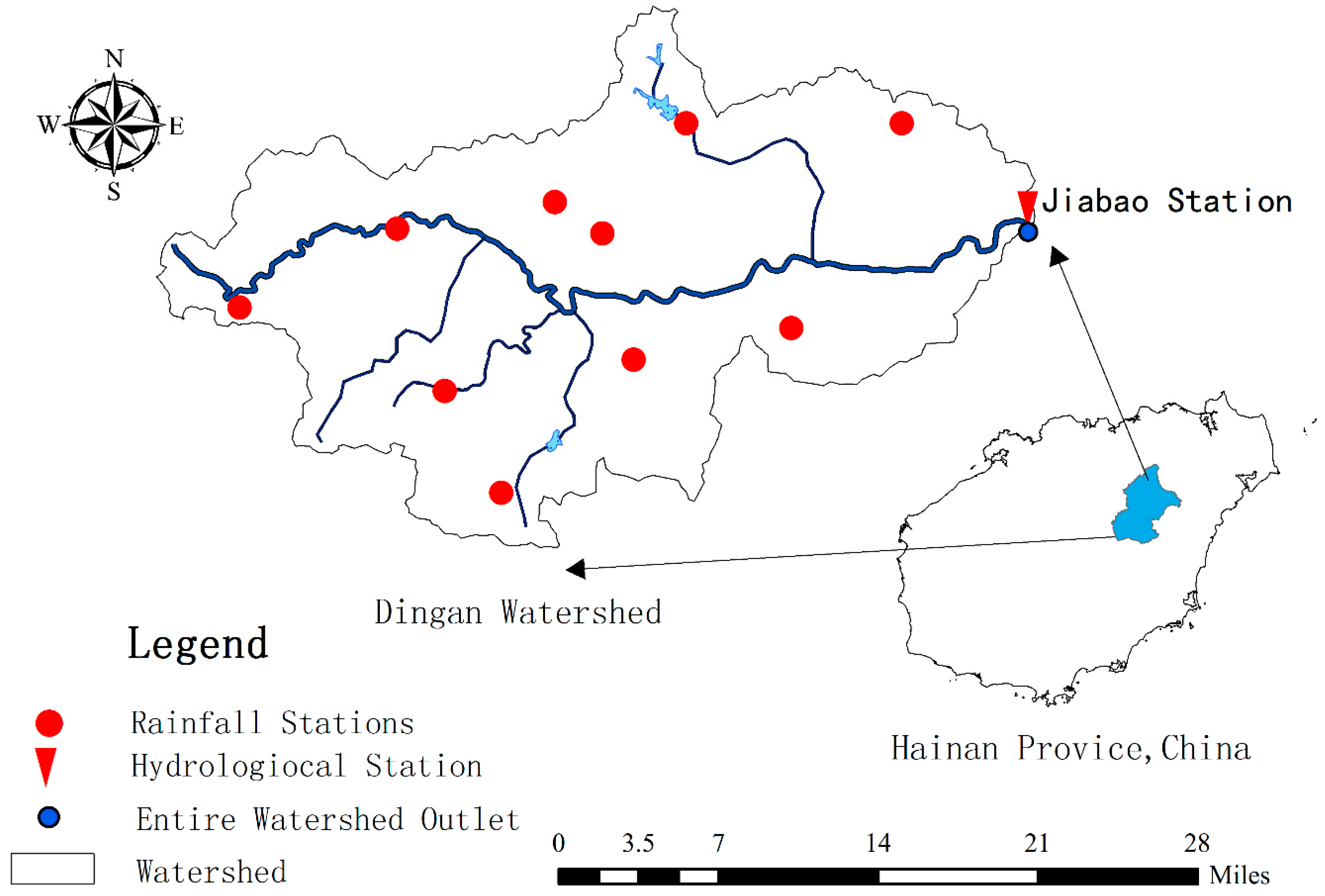
2. Study Area and Data

The Dingan River is located in the central region of Hainan Island in southern China. It is one of the major inputs to Wanquan River. Dingan River watershed is less affected by the water conservancy project as a headwaters area. The climate is dominated by tropical monsoon system with annual average temperature at 22 °C. The average annual precipitation is about 1639 mm, of which 70% is derived from typhoons and summer rainy season. The precipitation has a strong seasonal variability. About 70% to 90% of precipitation occurs during the period from May to November, which poses a great challenge on flood control.

In this paper, hourly rainfall data were collected in 11 rainfall stations in the Dingan River watershed (Figure 1). The corresponding observed hoult streamflow data were collected at Jiabao station at the outlet of the watershed. The digital elevation model (DEM) with a spatial resolution of 90 m is collected for sub-basin division. The watershed is selected because it is not disturbed by major water conservancy projects. Moreover, the data quality is good for both precipitation and streamflow with no missing value.

3. Methods

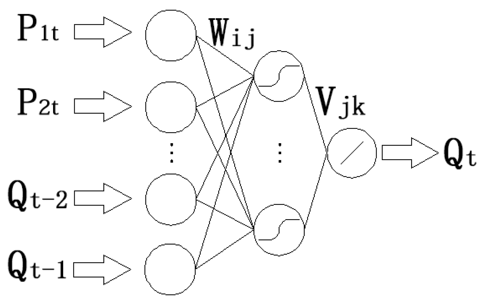
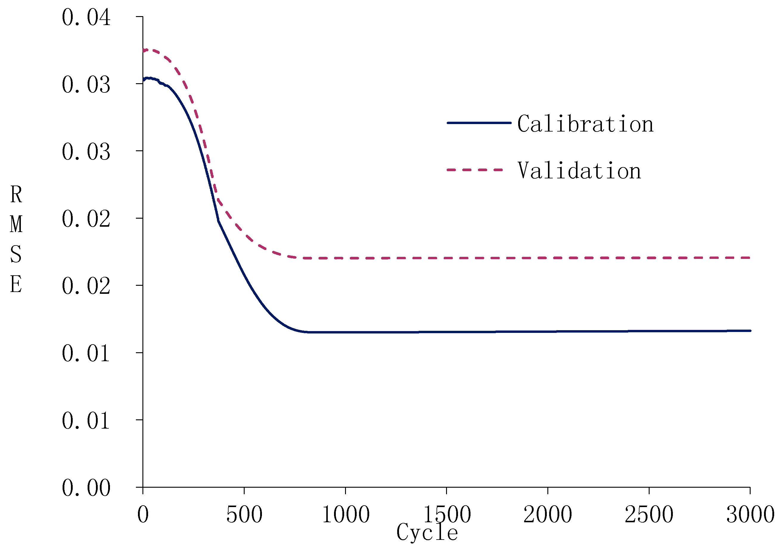
3.1. BP Neural Networks

BP neural network is a typical multilayer ANN, and uses Back-propagation to train the network [28]. The common structure used in hydrology to map all continuous nonlinear function consists of three layers: input layer, hidden layer, and output layer (Figure 2). A neural network is composed of massive nodes, with thresholds, activation functions and connection weights to characterize the architecture of the network [29]. The BP algorithm is a supervised learning method based on the steepest descent method to minimize the global error. The output errors are fed back through the network to modify the threshold values and connection weights. Finally, the optimal value can be obtained via iterative adjustment. Objective function takes root mean square error.

The neural network used in this paper has three layers and the number of nodes in hidden layer is determined by means of “trial and error”. It first employs the initial value calculated by Equation (1) and then less and more nodes are conducted to find the best performing one as the final value expressed as [30]:

$$\mathrm{Number} \mathrm{of} \mathrm{nodes} \mathrm{in} \mathrm{the} \mathrm{hidden} \mathrm{layer} = (\mathrm{input} \mathrm{number} + \mathrm{output} \mathrm{number}) \times \frac{2}{3}$$

(1)

The activation function of output layer is linear while the remaining layers are sigmoid functions. The outputs are obtained corresponding to the value of inputs using the formula as follow:

$$Q_k={\displaystyle \sum _{j=1}^m{V}_{jk}}\times F\left({\displaystyle \sum _{i=1}^n{p}_i\times W_{ij}}+b_{oj}\right)+b_{hk},k=t,t+1,\cdots ,N$$

(2)

where W_ij is the connection weight between ith node in the input layer and jth node in the hidden layer; V_jk is the connection weight between jth node in the hidden layer and kth node in the output layer; b_o and b_h are the bias, namely the threshold value, of nodes in the output layer and hidden layer respectively; P_i is the input of ith node; n, m and N are the number of nodes in the input layer, hidden layer and output layer, respectively; and F is the activation function of the hidden layer and in this paper is sigmoid function.

Various improved algorithms exist for building a BP neural network model [31,32,33]. In this study, three improved algorithms are selected:

(1) Momentum factor application [26,34]

The application of momentum factor is conducive to avoid oscillation when excessive correction happens and to speed up training on occasion it encounters flat regions of the error surface.

The biases and corresponding connection weights are adjusted based on the following formula:

$$\Delta W_{ij}(n)=-\beta \frac{\partial E(n)}{\partial W_{ij}}+\eta \Delta W_{ij}(n-1)$$

(3)

$$b_i(n)=-\beta \frac{\partial E(n)}{\partial b_i}+\eta b_i(n-1)$$

(4)

where W_ij is the connection weight between the ith node of preceding layer to jth node of this layer; n is the training times; E is the simulation error; β is the learning rate; η is the momentum factor; and b_i is the threshold value of ith node of this layer.

(2) Learning rate adaptation [35]

Real-time adjustment of learning rate of the network is essential to accelerate convergence. This paper selects the multiple of interval (2,5) of the distance from the calculation error to the target and interval (0.25,5) of the initial learning rate to construction proportional function, choosing the integer multiple of distance to form the double ratio coefficient array. When the multiple of distance is beyond the interval, it equals to the boundary value. The specific calculated function is expressed as follow:

$$\beta (n)=\{\begin{array}{c}{k}_{12}{\beta }_0,E(n)\le k_{11}{E}_{dis}\hfill \\ k_{22}{\beta }_0,k_{11}{E}_{dis}\le E(n)<k_{21}{E}_{dis}\hfill \\ \cdots \cdots \cdots \\ k_{(m-1)2}{\beta }_0,k_{(m-1)1}{E}_{dis}\le E(n)<k_{m1}{E}_{dis}\hfill \\ k_{m2}{\beta }_0,k_{m1}{E}_{dis}\le E(n)\hfill \end{array}$$

(5)

where n is the training times; E_dis is the target error; E is the current calculation error; β₀ is the initial learning rate; k_m1 is the mth double ratio coefficient to the target error; and k_m2 is the corresponding learning rate correction factor to the k_m1. k_m1 and k_m2 increase with the increase of m. The bigger is the double ratio coefficient of k_m1, the faster the learning rate of the next training phase becomes.

(3) Crossing validation [36,37]

Crossing validation is conducted to avoid over fitting by determining when the neural network begin to over-train. Over fitting happens when the neural network tries to fit the noise component of the data. Under this circumstance, it performs well over the training dataset, but shows poor results in forecasting. To apply the crossing validation, the data coverage period should be partitioned into three periods: calibration period (to calibrate the model parameters of the neural network), validation period (to stop the calibration phase when over training happens), and verification period (to test the accuracy of the simulation results). If the available dataset is too small for partitioning, the recommend solution is to stop the training when the objective error ceases to decrease significantly.

3.2. BP Neural Network Correction Algorithm

3.2.1. Traditional BP Neural Network Correction Algorithm

The traditional BP neural network correction algorithm is based on the principle of error auto regression. It is validated by the supervised learning method which requires actual value of variables to guide the training process. The inputs are the forecast error information of past N time periods, thus the real-time forecast error is calculated by the following equation:

$$e_t=Q_{p,t}-Q_{o,t}$$

(6)

$$e_{t+L}=F_{BP}(e_t,e_{t-1},\cdots ,e_{t-N+1})$$

(7)

$$Q_{p,t+L}^{\prime }=Q_{p,t+L}-e_{t+L}$$

(8)

where $e_t$ is the calculation error at t moment; $Q_{p,t}$ is the calculated value at t moment; $F_{BP}(\cdot )$ is the BP neural network method and its inputs; and $Q_{p,t+L}^{\prime }$ is the corrected calculated value at t moment.

In real-time correction, error autocorrelation in neighboring moment is at its strongest compared with each period. Therefore, prediction accuracy would decline as leading time increase. Intermediate variables such as sub-basin runoff yield and local inflow of main river channel generalized cannot be corrected by this method.

3.2.2. The Hydrological Model

The XAJ model chosen in this paper is a semi-distributed rainfall–runoff model developed in 1992 [38]. It is a typical conceptual hydrological model; the main feature of the model is the concept of runoff formation on repletion of storage. It means that, after the soil moisture context of aeration zone of the entire basin reaches field capacity, the runoff equals the rainfall excess. XAJ model has been proven as an effective model to simulate runoff in humid and semi-humid region. It has been applied over a large area including almost all of major river basins in China [39,40].

The study watershed is divided into eleven sub-basins and runoff of each sub-basin is computed. The outflow of each sub-basin (local inflow) is routed down the main river channel to the entire basin outlet concentrated by the Muskingum method. River concentration time of sub-basin in different positions is quite different. The outflow of upstream has a significant impact on the prediction results of downstream. Thus, we focus on the concentration part of XAJ model choosing the local inflow of main stream to be updated to improve the accuracy of flood forecasting.

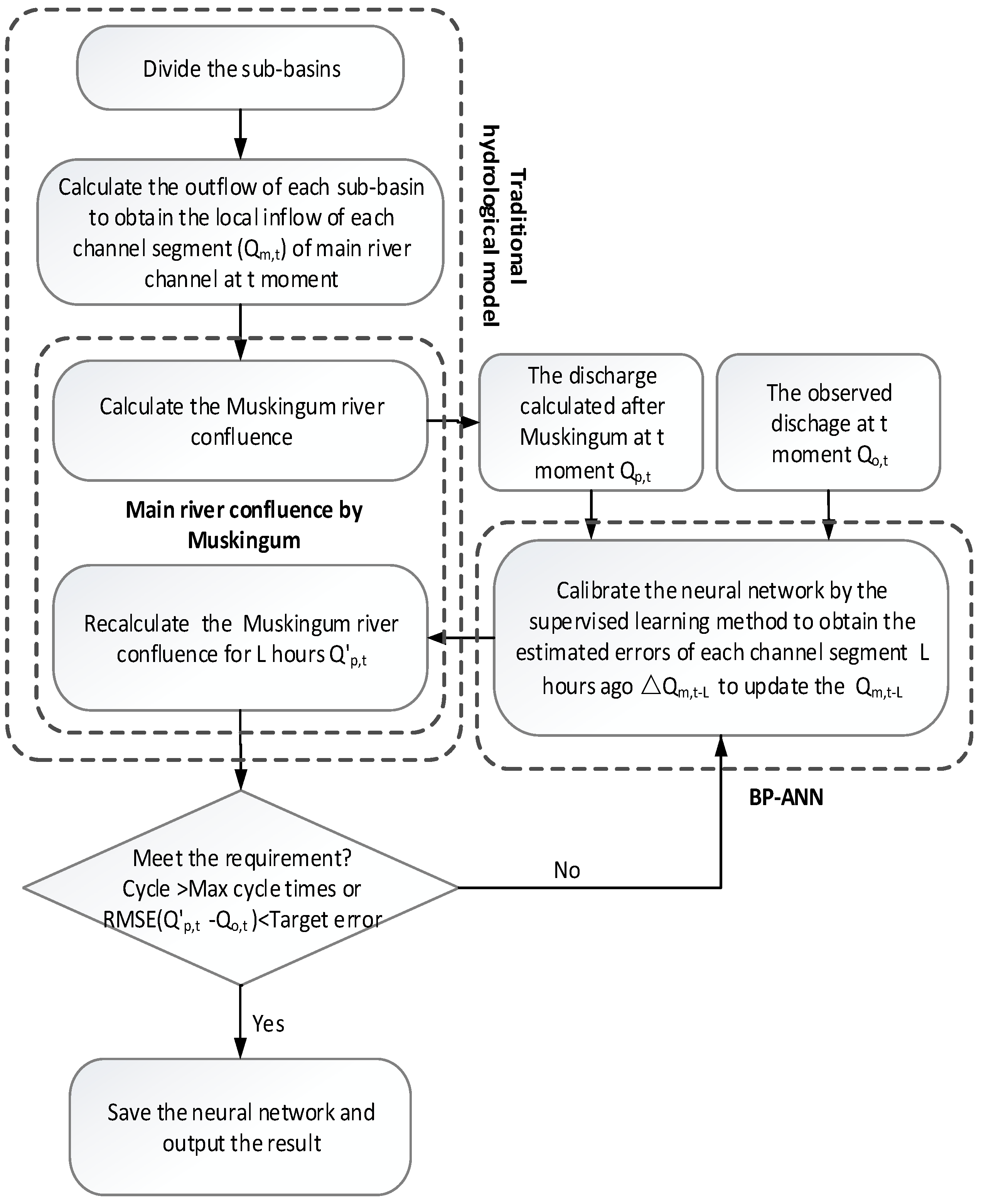
3.2.3. Apply BPC Algorithm in the Model

Considering that m channel segments of main river channel have local inflow, the inputs of BPC are the observed discharge and simulated discharge by XAJ model. The outputs are the estimated local inflow calculated errors of m channel segments of L hour ago. Then, Muskingum calculation process of L hours was repeated using the corrected local inflow. The calculation process can be expressed as follow (Figure 3):

$$\Delta Q_{m,t-\mathrm{L}}=F_{BPC}(Q_{p,t},Q_{o,t})$$

(9)

$$Q_{p,t+L}^{\prime }=F_{MSJG}(\Delta Q_{m,t-\mathrm{L}},Q_{m,t-L})$$

(10)

where $Q_{o,t}$ is the observed discharge at t moment; $Q_{p,t}$ is the calculated discharge after Muskingum at t moment; $F_{BPC}(\cdot )$ is the BPC method and its inputs; $\Delta Q_{m,t}$ is the estimated error of local inflow of mth channel segment calculated by BPC; $Q_{m,t}$ is the uncorrected local inflow of mth channel segment calculated by XAJ at t moment; $F_{MSJG}(\cdot )$ is the Muskingum method and its inputs; and $Q_{p,t+L}^{\prime }$ is the corrected local inflow of mth channel segment at t moment after L hours recalculation of Muskingum.

After the error $\Delta Q_p$ has been computed by the feed-forward process, the improved part of the backward propagation is as follows: Based on the characteristics of Muskingum linear calculus, it assumed that there is also linear relationship between local inflow error of channel segments and calculus eventually outflow error expressed as follow:

$$\Delta Q_{mo}-\Delta Q_m=k_m(Q_o-Q_p)$$

(11)

where $\Delta Q_{mo}$ is the ideal mth channel segment local inflow error; $\Delta Q_m$ is the calculation mth channel segment local inflow error; $Q_o$ is the observed discharge of the basin; $Q_p$ is the simulation discharge of the basin; and $k_m$ is the connection coefficient, in this paper is the linear ratio coefficient of the mth channel segment. Thus, the error function of mth output:

$$E_m=\frac{1}{2}{(\Delta Q_{mo}-\Delta Q_m)}^2$$

(12)

Considering the output layer of the neural network:

$$\Delta Q_m=V_{1m}{O}_1+V_{2m}{O}_2+\cdots +V_{nm}{O}_n+b_{om}$$

(13)

where $V_{jm}$ is the connection weight between jth hidden node and mth output node; $O_j$ is the output of jth hidden node; and $b_{om}$ is the bias of mth output nodes.

Therefore, the weights and the thresholds of each layer of the neural network can be modified by the formula based on mth channel segment local inflow error expressed as follow:

$$\Delta {\theta }_{om}=-\eta \frac{\partial E_m}{\partial {\theta }_{om}}=\eta k_m(Q_o-Q_p)$$

(14)

$$\Delta V_{jm}=-\eta \frac{\partial E_m}{\partial V_{jm}}=\eta k_m(Q_o-Q_p)O_j$$

(15)

$$\Delta {\theta }_{hj}=-\eta \frac{\partial E_m}{\partial {\theta }_{hj}}=\eta k_m(Q_o-Q_p)V_{jm}{O}_j\left(1-O_j\right)$$

(16)

$$\Delta W_{ij}=-\eta \frac{\partial E_m}{\partial W_{ij}}=\eta k_m(Q_o-Q_p)V_{jm}{O}_j\left(1-O_j\right)P_i$$

(17)

where $P_i$ is the ith input value.

Once the linear ratio coefficient (k) of each channel segment has been determined, the correction of BPC can achieve the intended purpose. $k_m$ can be obtained by three methods: (1) conducting linear fitting between each local inflow and streamflow at watershed outlet; (2) calculating the Muskingum convergence coefficient; and (3) instead of correcting the error based on the exactly ratio coefficient of each channel segment, the proportion of the correction can be determined by considering whether the direction of correction is correct. At the cost of a little convergence speed, the two speed convergence method can be adopted rather than the complete steepest descent method with an accurate $k_m$. Two different correction rates $k_{m1}$ and $k_{m2}$ are constructed to guide propagation. The improved formula expressed as follow:

$$k_m=\{\begin{array}{ll}{k}_{m1}& ,sign(\Delta Q_p)=sign(\Delta Q_{mp})\\ k_{m2}& ,sign(\Delta Q_p)\ne sign(\Delta Q_{mp})\end{array}$$

(18)

where $\Delta Q_p$ is the discharge calculation error of the outlet; $\Delta Q_{mp}$ is the estimated error of local inflow of mth channel segment calculated by BPC; and $sign(•)$ is the sign judgment function used to judge the positive and negative numbers.

Let $k_{m1}$ << $k_{m2}$. In this way, when the direction of calculation error of outlet discharge is consistent with that of the estimated error of mth channel segment local inflow calculated by BPC, small amplitude correction ($k_{m1}$) or large amplitude correction ($k_{m2}$) would be applied. Powerful automatic correction capability of BP neural network would ensure the corresponding weights and thresholds can be corrected in the right direction and the algorithm can converge well as long as there are sufficient data.

3.3. Evaluation Criteria

3.3.1. Correction Test Method

To analyze the characteristic of BPC, the single period correction test and real-time correction test were performed to verify the robustness and reliability of this method. In this paper, robustness is defined as the sustained correction effect of one time correction, including the prediction results of the subsequent periods should not be deteriorated. The reliability is defined as the approximation degree of measured flow and modified flow in actual forecasting circumstance, determining by statistical criteria such as the standards mentioned in Section 3.3.2.

The purpose of the single period correction test was to verify the robustness of BPC algorithm. The local inflow correction results of upstream channel segments would not fully appear until 7th h later because of flow concentration. It probably covers up the defects of the correction algorithm itself if we only focused on the current correction result. Therefore, all intermediate variables of concentration part of XAJ were saved. Once the past 1 h local inflows were corrected, we recalculated the Muskingum for the 2nd, 4th, and 6th h to test that whether the robustness of BPC can be guaranteed.

The purpose of the real-time correction test was to verify the reliability of BPC algorithm. It means that the forecasting results of discharge will be successive corrected at each period based on the observed value so as to give a better forecasting of next period. The real-time correction test simulates the situation in actual flood forecasting. Thus, the performance of the test can represent the correction effect to some extent in practical application.

3.3.2. Statistical Criteria

To evaluate the performance of measures used in forecasting and correction, multiple statistical criteria are selected to assess the fitness of simulation results of different schemes. The detailed equations are expressed as follow:

• Nash–Sutcliffe efficiency coefficient (NSE) [41]:

  $$NSE=1-{\displaystyle \sum _{i=1}^n\left[Q_s-Q_o\right]}/{\displaystyle \sum _{i=1}^n\left[Q_s-{\overline{Q}}_o\right]}$$

  (19)
• The relative error of peak flow:

  $$\delta Q=\left(Q_s-Q_o\right)/Q_o\times 100\%$$

  (20)
• The relative error of runoff depth:

  $$\delta R=\left(R_s-R_o\right)/R_o\times 100\%$$

  (21)

where n is the total number hours of a flood event; $Q_s$ and $Q_o$ are the simulated and observed peak flows, respectively; ${\overline{Q}}_o$ is the mean of observed discharge; and $R_s$ and $R_o$ are the total runoff depth calculated by simulation and observation, respectively.

4. Results and Discussion

Cross validation mentioned in Section 3.1 was applied to minimize the underlying relationship between inputs and outputs sufficiently and avoid over fitting at the same time. Based on this theory, the 20 flood events were divided into groups of seven, six, and seven for the three periods, respectively.

4.1. Model Construction and Testing

The Dingan River watershed was divided into 11 sub-basin using Thiessen polygon method. The outflow of each sub-basin was calculated and routed down along the main river channel to the watershed outlet. Seven channel segments had local inflow based on the overland flow calculations.

To correct the local inflows, the BPC method was applied to the concentration part of the XAJ model. The inputs of BPC were the discharge observed and simulated directly by XAJ model of the basin. The outputs were the one hour previous local inflow errors of the seven channel segments. The optimal number of hidden nodes was six through trial and error. The modified amplitude of each channel segment was limited to 20% for the security of hydrologic continuous

The neural network of BPC converged rapidly using the parameters in

Table 1. BPC parameter setting.

Parameter	Value
The initial learning rate	0.1
The initial momentum factor	0.15
Maximum cycle times	3000
Target root mean square error	0.01

and the optimal value was achieved at 845 times cycle (Figure 4). The error of the calibration data and the validation data were decreased consistently during the whole training phase. It implied that the neural network was trained well and might lead to a good simulation. To analyze the characteristic of BPC, the single period correction test and real-time correction test were performed to verify the robustness and reliability of this method.

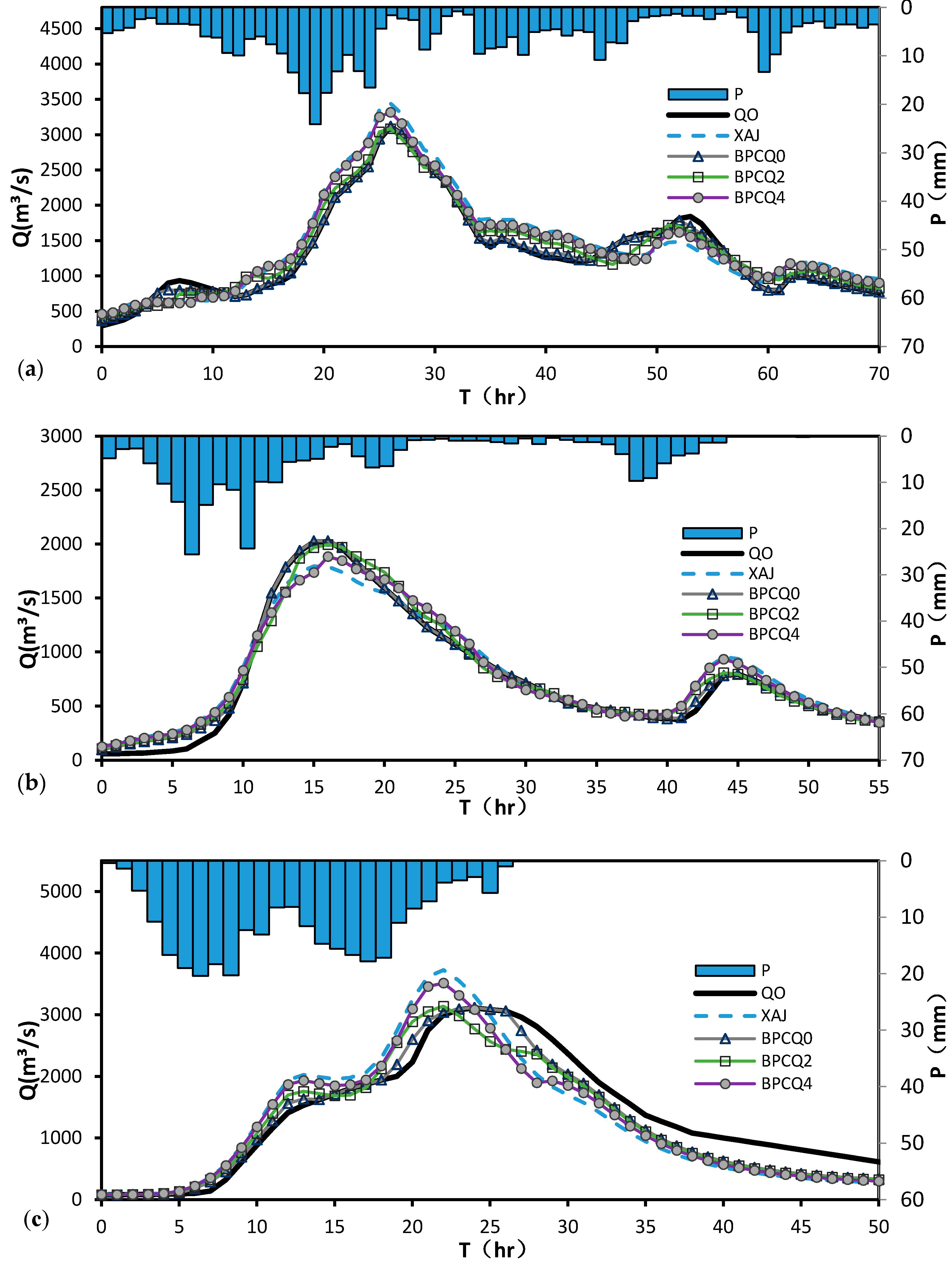
4.1.1. The Single Period Correction Test

All intermediate variables of concentration part of XAJ were saved. Once the past 1 h local inflows were corrected, we recalculated the Muskingum for the 2nd, 4th, and 6th h. During the recalculation process, there is no more correction. The results recorded as BPCQ0, BPCQ2 and BPCQ4 to represent the current, the preceding 2 h and 4 h outflow of the basin. The statistical results are shown in

Table 2. Single period correction performance for calibration period.

Flood Code	QO		XAJ			BPCQ0			BPCQ2			BPCQ4
	R	Q	δR	δQ	NSE	δR	δQ	NSE	δR	δQ	NSE	δR	δQ	NSE
	mm	m3/s	%	%	-	%	%	-	%	%	-	%	%	-
19981001	166.56	2110	10.16	−18.51	0.929	5.42	−3.63	0.987	6.30	−7.27	0.967	8.54	−14.89	0.943
19990518	52.18	1220	16.25	−16.52	0.932	9.10	-3	0.984	10.31	−14.11	0.954	14.74	−17.19	0.935
20000714	54.15	613	11.75	3.86	0.954	5.54	0.51	0.994	8.09	13.41	0.964	10.62	5.6	0.958
20000901	219.94	1070	2.44	−21	0.889	0.98	−7.91	0.965	1.16	−10.45	0.938	2.01	−16.98	0.909
20001009	680.71	3110	1.40	10.57	0.953	−0.72	0.23	0.997	−0.31	−0.85	0.986	0.58	6.64	0.968
20010515	31.71	527	10.50	1.23	0.635	10.28	0.44	0.824	8.42	−15.68	0.775	9.90	−4.28	0.673
20010825	296.18	3190	0.99	−5.31	0.976	−0.25	0.23	0.998	0.10	−1.71	0.991	0.63	−3.16	0.981
Mean	214.49	1691.43	7.64	11.00	0.895	4.61	2.28	0.964	4.96	9.07	0.939	6.71	9.82	0.910

Note: Mean is the average of absolute value, not directly added up for average.

,

Table 3. Single period correction performance for validation period.

Flood Code	QO		XAJ			BPCQ0			BPCQ2			BPCQ4
	R	Q	δR	δQ	NSE	δR	δQ	NSE	δR	δQ	NSE	δR	δQ	NSE
	mm	m3/s	%	%	-	%	%	-	%	%	-	%	%	-
20011021	119.59	1580	7.58	−30.47	0.845	2.24	−16.41	0.949	2.86	−18.14	0.93	4.89	−26.01	0.879
20020817	48.4	357	3.47	−4.36	0.653	3.84	−1.58	0.874	2.87	−6.44	0.824	2.95	−9.08	0.715
20050917	167.11	2020	7.98	−11.22	0.975	2.84	0.43	0.997	3.77	−1.23	0.987	6.15	−6.74	0.977
20051006	224.19	2560	1.85	10.54	0.877	1.90	0.12	0.96	1.56	−3.91	0.927	1.40	4.52	0.895
20071011	254.28	1620	−5.52	0.86	0.907	−1.60	0.24	0.977	−2.57	−6.44	0.958	−4.29	−1.88	0.929
20081003	87	1090	6.48	2.85	0.949	3.18	0.37	0.989	3.53	−9.73	0.972	5.14	−1.41	0.957
Mean	150.10	1537.83	5.48	10.05	0.868	2.60	3.19	0.958	2.86	7.65	0.933	4.14	8.27	0.892

Note: Mean is the average of absolute value, not directly added up for average.

and

Table 4. Single period correction performance for verification period.

Flood Code	QO		XAJ			BPCQ0			BPCQ2			BPCQ4
	R	Q	δR	δQ	NSE	δR	δQ	NSE	δR	δQ	NSE	δR	δQ	NSE
	mm	m3/s	%	%	-	%	%	-	%	%	-	%	%	-
20081012	434.26	2810	1.89	−0.21	0.971	0.34	0.22	0.997	0.48	−5.27	0.984	1.00	4.39	0.974
20090922	320.15	1860	5.67	−1.96	0.951	0.54	0.3	0.993	1.53	7.4	0.979	3.62	4.63	0.959
20101012	563.04	3250	1.11	1.46	0.971	−1.26	0.19	0.997	−1.34	−2.13	0.988	−0.18	−1.77	0.979
20110923	549.14	2460	−0.09	19.59	0.854	−3.11	0.35	0.974	−2.21	3.33	0.952	−1.18	11.85	0.907
20111103	198.23	2630	0.44	14.07	0.962	−3.75	0.14	0.994	−3.68	2.06	0.99	−1.68	9.74	0.98
20120615	60.86	526	18.81	9.45	0.812	8.82	0.4	0.928	12.18	9.44	0.883	15.97	7.58	0.851
20131109	249.43	3110	−7.25	19.82	0.882	−7.95	0.17	0.968	−9.04	0.85	0.943	−8.04	12.99	0.907
Mean	339.30	2378.00	5.04	9.51	0.915	3.68	0.25	0.979	4.35	4.35	0.960	4.52	7.56	0.937

Note: Mean is the average of absolute value, not directly added up for average.

.

The high average NSE in Table 2 indicated that the forecasting results of XAJ were relatively good. However, the values of δR and δQ of some flood events are unsatisfactory and could be improved. The correction effect comparison of BPCQ0, BPCQ2 and BPCQ4 were analyzed.

In term of mean δR, the results in Table 2, Table 3 and Table 4 indicated that the BPC method could truly improve the accuracy of prediction of water balance and had a continuous effect as BPQC4 was still much better than the original prediction (XAJ). The mean δQ represents the accuracy of the flood peak forecasting. The calculated flood peak is always an essential prediction factor in flood forecasting as it can distinguish the amplitude of flood event and directly affect flood control, flood rescue, reservoir operation, and other measures. δQ decreased significantly, which indicated that the proposed method could improve flood forecasting. After correction, the mean NSE of the three total periods were obviously improved compared with the previous ones. The increased NSE value shows a better fitness between simulation and observed records.

Three hydrographs were selected to display the correction effect in total phases (see Figure 5). The results implied the correction algorithm was effective and stability.

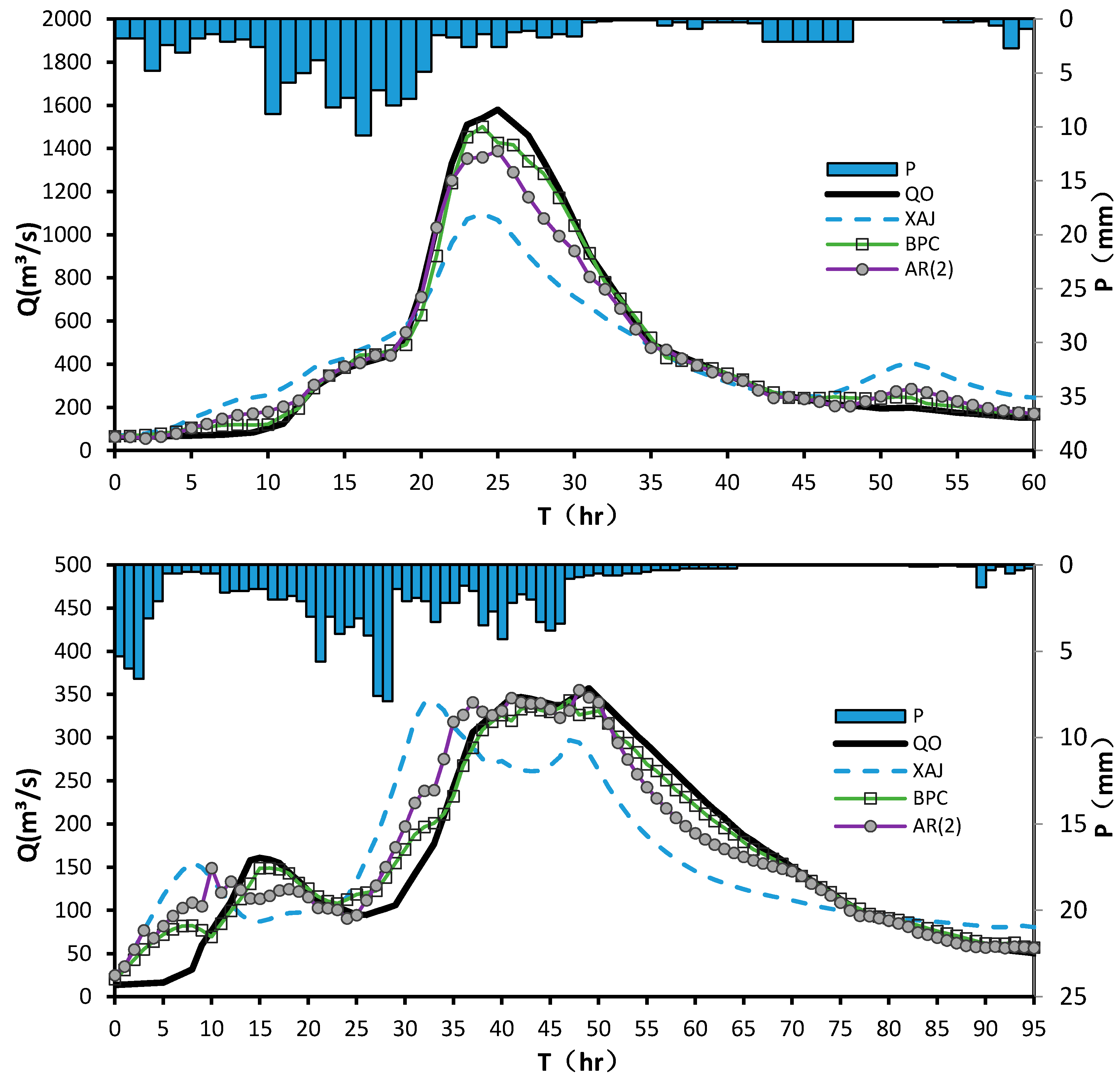
4.1.2. The Real-Time Correction Test

The neural network used in this test was calibrated by the single period test performed above, thus there was no need to divide the data into calibration, validation and verification period. The real-time correction test updates the local inflows of main river channel at each period, successively, which is different from the single period correction used in calibration phase. It can greatly save the amount of datasets required as the flood events selected to conduct single period correction can be reused in this test. Therefore, all flood events were simulated to gain a comprehensive cognition of BPC method. For comparison, a second-order autoregression AR(2) algorithm was also calculated.

Table 5. Comparison between original model results and real-time correction results of BPC and AR(2).

Flood Code	QO		XAJ			BPC			AR(2)
	R	Q	δR	δQ	NSE	δR	δQ	NSE	δR	δQ	NSE
	mm	m3/s	%	%	-	%	%	-	%	%	-
19981001	166.56	2110	10.16	−18.51	0.929	3.68	−4.77	0.992	2.59	0.13	0.988
19990518	52.18	1220	16.25	−16.52	0.932	5.48	−4.24	0.981	4.94	−1.15	0.974
20000714	54.15	613	11.75	3.86	0.954	4.10	0.16	0.991	0.76	5.43	0.988
20000901	219.94	1070	2.44	−21	0.889	0.82	2.58	0.977	−0.26	−2.82	0.974
20001009	680.71	3110	1.40	10.57	0.953	0.99	−0.95	0.996	−0.48	−1.95	0.996
20010515	31.71	527	10.50	1.23	0.635	7.10	−0.25	0.919	14.13	27.47	0.755
20010825	296.18	3190	0.99	−5.31	0.976	0.24	−0.83	0.997	−0.06	4.95	0.999
20011021	119.59	1580	7.58	−30.47	0.845	2.15	−4.97	0.992	−1.02	−12.09	0.975
20020817	48.4	357	3.47	−4.36	0.653	3.02	−3.89	0.973	4.17	−0.56	0.92
20050917	167.11	2020	7.98	−11.22	0.975	2.50	−1.9	0.997	2.51	−2.13	0.989
20051006	224.19	2560	1.85	10.54	0.877	2.80	0.98	0.974	2.32	7.21	0.968
20071011	254.28	1620	−5.52	0.86	0.907	−0.35	0.57	0.99	−1.18	3.93	0.98
20081003	87	1090	6.48	2.85	0.949	2.61	−3.28	0.992	3.26	3.81	0.988
20081012	434.26	2810	1.89	−0.21	0.971	0.81	−2.17	0.995	0.14	2.08	0.996
20090922	320.15	1860	5.67	−1.96	0.951	1.47	5.31	0.996	−0.24	−0.65	0.993
20101012	563.04	3250	1.11	1.46	0.971	0.71	2.4	0.997	−0.92	4.55	0.992
20110923	549.14	2460	−0.09	19.59	0.854	−1.02	4.76	0.986	−4.67	1.98	0.987
20111103	198.23	2630	0.44	14.07	0.962	0.18	0.58	0.997	−3.80	−4.24	0.994
20120615	60.86	526	18.81	9.45	0.812	7.15	7.74	0.964	5.29	3.04	0.961
20131109	249.43	3110	−7.25	19.82	0.882	−1.82	−0.33	0.991	−5.53	8.64	0.975
Mean	238.86	1885.65	6.08	10.19	0.894	2.45	2.63	0.985	2.91	4.94	0.970

Note: Mean is the average of absolute value, not directly added up for average.

shows that the BPC method passed the real-time correction test. The results indicated that significant improvement had been achieved in respects of mean NSE, δR and δQ after correction by BPC and AR(2), respectively. The correction effect of AR(2) was very good for prediction of real-time, but the accuracy of BPC was slightly better. In addition, the application of BPC in XAJ makes the real time correction possible without losing the leading time. Above all, the BPC method is an new alternative choice to AR(2), ensemble Kalman filter, dynamic system response curve, etc. to correct flood forecasting [42,43,44].

Two hydrographs are presented to display the correction effect of BPC and AR(2) method. Figure 6 shows that the correction accuracy of BPC was better.

4.2. Strengths and Shortcomings

Although the robustness and reliability is checked in Section 4.1, more indicators need to be taken into consideration to comprehensively understand the strengths and drawbacks of BPC. In this paper, we further evaluated the performance of BPC by comparing it with other correction methods in terms of three indicators: simplicity, computation time and data demand.

Simplicity is one of the most important characteristics for hydrological models as it largely influences the application of models. The BPC method was incorporated into traditional hydrological model, which makes it more complex than BP and AR(2) method. The number of parameters includes three parts: the parameters of traditional hydrological model, the parameters of BP method, and the connection coefficients $k_{m1}$ and $k_{m2}$. The parameters of first part need to be calibrated separately. After $k_{m1}$ and $k_{m2}$ have been set, the parameters of the BP method can be calibrated automatically by the supervised learning method and learning rate adaptation method. The number of hidden nodes is determined by trial and error. In general, simple models are more likely to be popularized and applied. However, in the case of high requirement of flood prediction, complex methods such as BPC are probably more practical.

The calibration time for neural networks to converge is an important criterion for model evaluation. The training phase of the BPC method partly depended on the intermediate variables and outputs of the XAJ model. The intermediate variables and outputs calculated by XAJ model have certain physical meaning and are more reasonable. Thus, it can largely decrease the calibration time of the neural network. The number of cycles in the calibration phase in Dingan River watershed is 845 times for BPC to converge while it usually takes nearly 10,000 times for traditional BP method. Once the neural network has calibrated, it can be used to correct the flood prediction and no further effort shall be devoted to it.

As a data-driven forecasting method, the success of BPC requires ample data. In the neural network calibration phase, the data available need to be divided into three parts. High quality and quantity of data can largely improve the accuracy of correction by BPC. With the continuous improvement of hydrometry technology, more accurate and reliable data will become accessible in the future. Thus, the BPC method could play more important value in hydrologic forecasting.

5. Conclusions

Flood forecasting based on hydrological models is one of the essential non-engineering measures. The prediction accuracy has a large impact on the flood control and rescue. The forecasting errors of preceding periods may have significant negative effect on the prediction of following periods, thus searching for better methods to correct the forecasting error become a research hotspots for hydrologists. To handle these problems, we had proposed a new BP neural network correction algorithm in this paper and gained the following conclusion:

(1)

This method is based on the BP neural network and is incorporated into a traditional hydrological model, thus it combines the advantages of both models. It could obviously correct the forecasting error of XAJ model and increase the forecasting accuracy without losing the leading time.

(2)

The performance of suggested BPC method has been checked by the single period correction test and real-time correction test. The results of tests implied that this method is stable and reliable.

(3)

Although the BPC method increased the number of parameters, most parameters can be calibrated automatically by the supervised learning method and learning rate adaptation method. In addition, it can largely shorten the computation time for calibration.

(4)

As a data-driven method, The BPC method is especially effective for the areas with adequate data, and the accuracy of correction was superior to the widespread AR(2) method.

References

1. Rumelhart, D.E.; Hinton, G.E.; Williams, R.J. Learning internal representation by back propagation. In Parallel Distributed Processing: Exploration in the Microstructure of Cognition; The MIT Press: Cambridge, MA, USA, 1986; Volume 1. [Google Scholar]
2. Wang, Z.; Lai, C.; Chen, X.; Yang, B.; Zhao, S.; Bai, X. Flood hazard risk assessment model based on random forest. J. Hydrol. 2015, 527, 1130–1141. [Google Scholar] [CrossRef]
3. Werner, M.; Reggiani, P.; De Roo, A.; Bates, P.; Sprokkereef, E. Flood forecasting and warning at the river basin and at the European scale. Nat. Hazards 2005, 36, 25–42. [Google Scholar] [CrossRef]
4. Jiang, P.; Gautam, M.R.; Zhu, J.; Yu, Z. How well do the gcms/rcms capture the multi-scale temporal variability of precipitation in the southwestern united states? J. Hydrol. 2013, 479, 75–85. [Google Scholar] [CrossRef]
5. Yu, Z.; Jiang, P.; Gautam, M.R.; Zhang, Y.; Acharya, K. Changes of seasonal storm properties in california and nevada from an ensemble of climate projections. J. Geophys. Res. Atmos. 2015, 120, 2676–2688. [Google Scholar] [CrossRef]
6. Jiang, P.; Yu, Z.; Gautam, M.R.; Acharya, K. The spatiotemporal characteristics of extreme precipitation events in the western united states. Water Resour. Manag. 2016, 30, 4807–4821. [Google Scholar] [CrossRef]
7. Moore, R.J.; Bell, V.A.; Jones, D.A. Forecasting for flood warning. C. R. Geosci. 2005, 337, 203–217. [Google Scholar] [CrossRef]
8. Young, P.C. Advances in real-time flood forecasting. Philos. Trans. A Math. Phys. Eng. Sci. 2002, 360, 1433–1450. [Google Scholar] [CrossRef] [PubMed]
9. Cloke, H.; Pappenberger, F. Ensemble flood forecasting: A review. J. Hydrol. 2009, 375, 613–626. [Google Scholar] [CrossRef]
10. Weimin, B.; Wei, S.; Simin, Q. Flow updating in real-time flood forecasting based on runoff correction by a dynamic system response curve. J. Hydrol. Eng. 2013, 19, 747–756. [Google Scholar] [CrossRef]
11. Hosseini, S.M.; Mahjouri, N. Integrating support vector regression and a geomorphologic artificial neural network for daily rainfall-runoff modeling. Appl. Soft Comput. 2016, 38, 329–345. [Google Scholar] [CrossRef]
12. Tingsanchali, T.; Gautam, M.R. Application of tank, nam, arma and neural network models to flood forecasting. Hydrol. Process. 2000, 14, 2473–2487. [Google Scholar] [CrossRef]
13. Shi, P.; Hou, Y.; Xie, Y.; Chen, C.; Chen, X.; Li, Q.; Qu, S.; Fang, X.; Srinivasan, R. Application of a swat model for hydrological modeling in the xixian watershed, china. J. Hydrol. Eng. 2013, 18, 1522–1529. [Google Scholar] [CrossRef]
14. Si, W.; Bao, W.; Jiang, P.; Zhao, L.; Qu, S. A semi-physical sediment yield model for estimation of suspended sediment in loess region. Int. J. Sediment Res. 2015, in press. [Google Scholar]
15. Si-min, Q.; Wei-min, B.; Peng, S.; Zhongbo, Y.; Peng, J. Water-stage forecasting in a multitributary tidal river using a bidirectional muskingum method. J. Hydrol. Eng. 2009, 14, 1299–1308. [Google Scholar] [CrossRef]
16. Vrugt, J.A.; Gupta, H.V.; Bouten, W.; Sorooshian, S. A shuffled complex evolution metropolis algorithm for estimating posterior distribution of watershed model parameters. Calibration Watershed Models 2003, 39, 105–112. [Google Scholar]
17. Wu, C.; Chau, K.; Fan, C. Prediction of rainfall time series using modular artificial neural networks coupled with data-preprocessing techniques. J. Hydrol. 2010, 389, 146–167. [Google Scholar] [CrossRef]
18. De Vos, N.; Rientjes, T. Multiobjective training of artificial neural networks for rainfall-runoff modeling. Water Resour. Res. 2008, 44, W08434. [Google Scholar] [CrossRef]
19. Jain, A.; Srinivasulu, S. Development of effective and efficient rainfall-runoff models using integration of deterministic, real-coded genetic algorithms and artificial neural network techniques. Water Resour. Res. 2004, 40, W04302. [Google Scholar] [CrossRef]
20. Aqil, M.; Kita, I.; Yano, A.; Nishiyama, S. A comparative study of artificial neural networks and neuro-fuzzy in continuous modeling of the daily and hourly behaviour of runoff. J. Hydrol. 2007, 337, 22–34. [Google Scholar] [CrossRef]
21. Tiwari, M.K.; Chatterjee, C. Development of an accurate and reliable hourly flood forecasting model using wavelet–bootstrap–ann (WBANN) hybrid approach. J. Hydrol. 2010, 394, 458–470. [Google Scholar] [CrossRef]
22. Elsafi, S.H. Artificial neural networks (ANNS) for flood forecasting at dongola station in the River Nile, Sudan. Alexandria Eng. J. 2014, 53, 655–662. [Google Scholar] [CrossRef]
23. Hartmann, H.; Becker, S.; King, L.; Jiang, T. Forecasting water levels at the yangtze river with neural networks. Erdkunde 2008, 62, 231–243. [Google Scholar] [CrossRef]
24. Maier, H.R.; Dandy, G.C. Neural networks for the prediction and forecasting of water resources variables: A review of modelling issues and applications. Environ. Model. Softw. 2000, 15, 101–124. [Google Scholar] [CrossRef]
25. Bebis, G.; Georgiopoulos, M. Feed-forward neural networks. IEEE Potentials 1994, 13, 27–31. [Google Scholar] [CrossRef]
26. Govindaraju, R.S. Artificial neural networks in hydrology. I: Preliminary concepts. J. Hydrol. Eng. 2000, 5, 115–123. [Google Scholar]
27. Fares, A.; Awal, R.; Michaud, J.; Chu, P.-S.; Fares, S.; Kodama, K.; Rosener, M. Rainfall-runoff modeling in a flashy tropical watershed using the distributed HL-RDHM model. J. Hydrol. 2014, 519, 3436–3447. [Google Scholar] [CrossRef]
28. Fausett, L. Fundamentals of Neural Networks: Architectures, Algorithms, and Applications; Prentice-Hall, Inc.: Upper Saddle River, NJ, USA, 1994. [Google Scholar]
29. Parks, R.W.; Levine, D.S.; Long, D.L. Fundamentals of Neural Network Modeling: Neuropsychology and Cognitive Neuroscience; MIT Press: London, UK, 1998. [Google Scholar]
30. Han, D.; Kwong, T.; Li, S. Uncertainties in real-time flood forecasting with neural networks. Hydrol. Process. 2007, 21, 223–228. [Google Scholar] [CrossRef]
31. Yao, X. A review of evolutionary artificial neural networks. Int. J. Intell. Syst. 1993, 8, 539–567. [Google Scholar] [CrossRef]
32. Zhu, M.-L.; Fujita, M.; Hashimoto, N. Application of neural networks to runoff prediction. In Stochastic and Statistical Methods in Hydrology and Environmental Engineering; Springer: Norwell, MA, USA, 1994; pp. 205–216. [Google Scholar]
33. Yu, X.-H.; Chen, G.-A. Efficient backpropagation learning using optimal learning rate and momentum. Neural Netw. 1997, 10, 517–527. [Google Scholar] [CrossRef]
34. Hassoun, M.H. Fundamentals of Artificial Neural Networks; MIT Press: London, UK, 1995. [Google Scholar]
35. Huijuan, F.; Jiliang, L.; Fei, W. Fast learning in spiking neural networks by learning rate adaptation. Chin. J. Chem. Eng. 2012, 20, 1219–1224. [Google Scholar]
36. Senthil Kumar, A.; Sudheer, K.; Jain, S.; Agarwal, P. Rainfall-runoff modelling using artificial neural networks: Comparison of network types. Hydrol. Process. 2005, 19, 1277–1291. [Google Scholar] [CrossRef]
37. Rang, M.S.; Kang, M.G.; Park, S.W.; Lee, J.J.; Yoo, R.H. Application of Grey Model and Artificial Neural Networks to Flood Forecasting. J. Am. Water Resour. Assoc. 2006, 42, 473–486. [Google Scholar] [CrossRef]
38. Zhao, R. The xinanjiang model applied in China. J. Hydrol. 1992, 135, 371–381. [Google Scholar]
39. Yao, C.; Zhang, K.; Yu, Z.; Li, Z.; Li, Q. Improving the flood prediction capability of the xinanjiang model in ungauged nested catchments by coupling it with the geomorphologic instantaneous unit hydrograph. J. Hydrol. 2014, 517, 1035–1048. [Google Scholar] [CrossRef]
40. Yuan, F.; Ren, L. Application of the xinanjiang vegetation—Hydrology model to streamflow simulation over the Hanjiang river basin, China. IAHS-AISH Publ. 2009, 326, 63–69. [Google Scholar]
41. Yapo, P.O.; Gupta, H.V.; Sorooshian, S. Automatic calibration of conceptual rainfall-runoff models: Sensitivity to calibration data. J. Hydrol. 1996, 181, 23–48. [Google Scholar] [CrossRef]
42. Komma, J.; Bloschl, G.; Reszler, C. Soil moisture updating by ensemble kalman filtering in real-time flood forecasting. J. Hydrol. 2008, 357, 228–242. [Google Scholar] [CrossRef]
43. Chen, H.; Yang, D.; Hong, Y.; Gourley, J.J.; Zhang, Y. Hydrological data assimilation with the ensemble square-root-filter: Use of streamflow observations to update model states for real-time flash flood forecasting. Adv. Water Resour. 2013, 59, 209–220. [Google Scholar] [CrossRef]
44. Si, W.; Bao, W.; Gupta, H.V. Updating real-time flood forecasts via the dynamic system response curve method. Water Resour. Res. 2015, 51, 5128–5144. [Google Scholar] [CrossRef]
Figure 1. Distribution of hydrological stations network in Dingan River watershed.
Water 09 00048 g001
Figure 2. Configuration of a three-layer BP neural network.
Water 09 00048 g002
Figure 3. The flowchart of the BPC algorithm applied to the traditional hydrological model.
Water 09 00048 g003
Figure 4. Global error variation of neural network cross validation process.
Water 09 00048 g004
Figure 5. Single period correction performance comparison of different models: (a) flood 20001009 of calibration period; (b) flood 20050917 of validation period; and (c) flood 20131109 of verification period.
Water 09 00048 g005
Figure 6. Real-time correction performance comparison of BPC and AR(2) of floods 20011021 and 20020817.
Water 09 00048 g006