
3D CFD Modeling of Local Scouring, Bed Armoring and Sediment Deposition


1
Water Management Research Group, Hungarian Academy of Science—Budapest University of Technology and Economics, Műegyetem rakpart 3, H-1111 Budapest, Hungary
2
Department of Hydraulic and Water Resources Engineering, Budapest University of Technology and Economics, Műegyetem rakpart 3, H-1111 Budapest, Hungary
3
Department of Hydraulic and Environmental Engineering, Norwegian University of Science and Technology, S. P. Andersens vei 5, 7491 Trondheim, Norway
*
Author to whom correspondence should be addressed.
Water 2017, 9(1), 56; https://doi.org/10.3390/w9010056
Submission received: 14 October 2016
/
Revised: 3 January 2017
/
Accepted: 9 January 2017
/
Published: 17 January 2017
(This article belongs to the Special Issue Watershed Sediment Process)
Abstract
:3D numerical models are increasingly used to simulate flow, sediment transport and morphological changes of rivers. For the simulation of bedload transport, the numerical flow model is generally coupled with an empirical sediment transport model. The application range of the most widely used empirical models is, however, often limited in terms of hydraulic and sedimentological features and therefore the numerical model can hardly be applied to complex situations where different kinds of morphological processes take place at the same time, such as local scouring, bed armoring and aggradation of finer particles. As a possible solution method for this issue, we present the combined application of two bedload transport formulas that widens the application range and thus gives more appropriate simulation results. An example of this technique is presented in the paper by combining two bedload transport formulas. For model validation, the results of a laboratory experiment, where bed armoring, local scouring and local sediment deposition processes occurred, were used. The results showed that the combined application method can improve the reliability of the numerical simulations.
1. Introduction
The investigation of riverine sediment transport is of major interest to researchers. There are numerous empirically derived bedload transport formulas which are used to model bedload discharge, developed usually for a given narrow range of flow and sediment regimes. However, due to the complex nature of the sediment motion, especially the bedload transport, there is no generally applicable method to describe the related morphodynamic processes. A comprehensive collection of the most widely applied formulas can be found in Sedimentation Engineering Handbook [1]. The collection contains the most relevant sediment transport models, such as the ones from Meyer-Peter and Müller [2], Einstein [3], Ashida and Michiue [4], Parker, Klingeman and McLean [5], surface-based relation of Parker [6], two-fraction relation of Wilcock and Kenworthy [7], surface-based relation of Wilcock and Crowe [8], relation of Wu et al. [9], and that of Powell et al. [10]. The summary [1] provides a short description of the hydraulic and sediment conditions of the experiments for which the given bedload formulas were developed. These conditions thus actually define the morphological features, for which the application of the given formula is recommended. In other words, the hydraulic and sediment conditions of the benchmark experiments determine the applicability limits of the formulas, primarily regarding to the sediment content. For example, the Meyer-Peter and Müller [2] formula was verified for uniform coarser grains, focusing on the alpine flows in Switzerland. The relation of Einstein was developed also for uniform gravels. According to Yang and Wan [11], its application is more reliable for local sediment motion calculation, instead of modeling larger river sections. The first model for non-uniform mixture was the relation of Ashida and Michiue [4]. One of the known limitations of the formula is that it is not recommended for natural gravel-bed rivers [1].
In the case of the van Rijn formula, [12], the benchmark flume tests and experimental data for calibration and validation were carried out with finer bed materials [2,13,14,15,16,17]. Thus, based on the morphodynamic features of these measurements, the recommended application range of the formula is limited only for sand (<2 mm) fractions. In contrast, the relations of Wilcock and Crowe [8] were developed for coarser, sand-gravel mixture (0.5 mm–64 mm) [18]. Similarly, the application of each sediment transport model is also limited.
However, in complex flow and morphological cases—e.g., situations where different morphodynamic processes like scouring, bed armoring and aggradation take place at the same time—a less limited sediment transport approximation method would be needed, particularly when sediment transport of varied—both in time and space—bedload composition occurs, e.g., in river sections with river training structures, like groin fields. In such cases, the applicability limits of the existing sediment transport formulas still set back the accuracy of the numerical modeling. Because of this, for reliable morphological modeling, a more complex description would be expected than the above-mentioned formulas separately offer.
In turn, according to the basic inspiration of the authors, the accuracy of the sediment transport modeling can be optimized by the coupled application of existing sediment transport equations. The main advantage of the concept is that the user does not have to choose one sediment transport formula, rather the model formulates the most reliable sediment transport calculation in the given sediment regime.
The basic challenge in this study was to simulate the morphodynamic changes measured in a flume experiment in Török et al. [19], where the scouring process takes place over time, and is influenced by bed armoring. For such a complex sediment transport calculation purpose, the Wilcock and Crowe [8] formula is recommended. However, bed aggradation and degradation of the fine eroded materials also appear; these phenomena can be taken into account by the van Rijn [12] model. Thus, theoretically, the coupled application of these two models became justified and so a more reliable sediment transport modeling is assumed. The main goal of this research is to improve this hypothesis statement. The aim of this paper is to demonstrate the capabilities of a 3D numerical flow and sediment transport model which applies a combined bedload transport description using two distinct empirical equations concurrently, if the spatial distribution of the bed material composition is strongly inhomogeneous.
We present: (i) a thorough introduction of the laboratory experiments; (ii) the numerical model setup and implementation of the sediment transport formulas and (iii) a summary description of the benefits of the coupled application method based on the numerical model results.
2. Laboratory Experiments
2.1. Experimental Setup and Measurement Procedure
The flume experiments of Török et al. [19] were used for numerical model validation purposes.
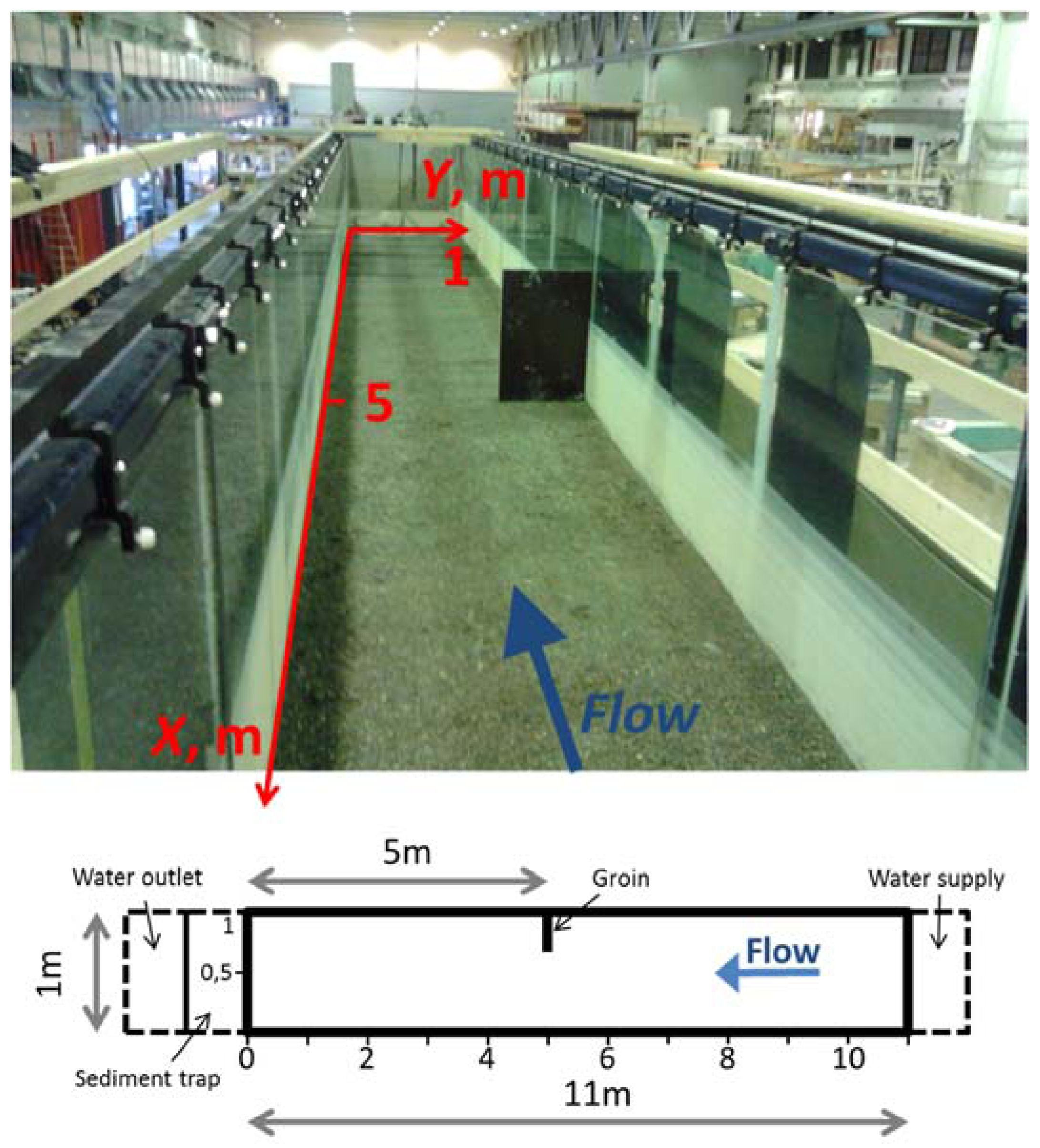
The laboratory flume, in which the experiments were performed, is an 11 m long and 1 m wide channel. In the flume, a 0.33 m long obstacle was placed perpendicular to the flow, 5 m far from the end of the flume. A local coordinate system has been added, which can be seen in Figure 1.
The measurement was performed at three different constant discharges (see Table 1). First, the lowest discharge was run until no substantial bed change could be detected, representing the transport equilibrium state. Then, without any disturbance of the developed equilibrium state, the higher discharge started and was run until the second equilibrium state. Finally, the highest discharge was run in the same way. The measured main hydraulic features for each discharge are presented in Table 1. Herein, Q is the flow discharge, havg is the water depth at the outlet, vavg is the averaged flow velocity, Fr is the Froude number, Re is the Reynolds number, τavg is the averaged bed shear stress, estimated as described later on and Sbed is the bed slope. The variables show that the flow was subcritical (Fr < 1) and turbulent (Re > 40,000) in every case.
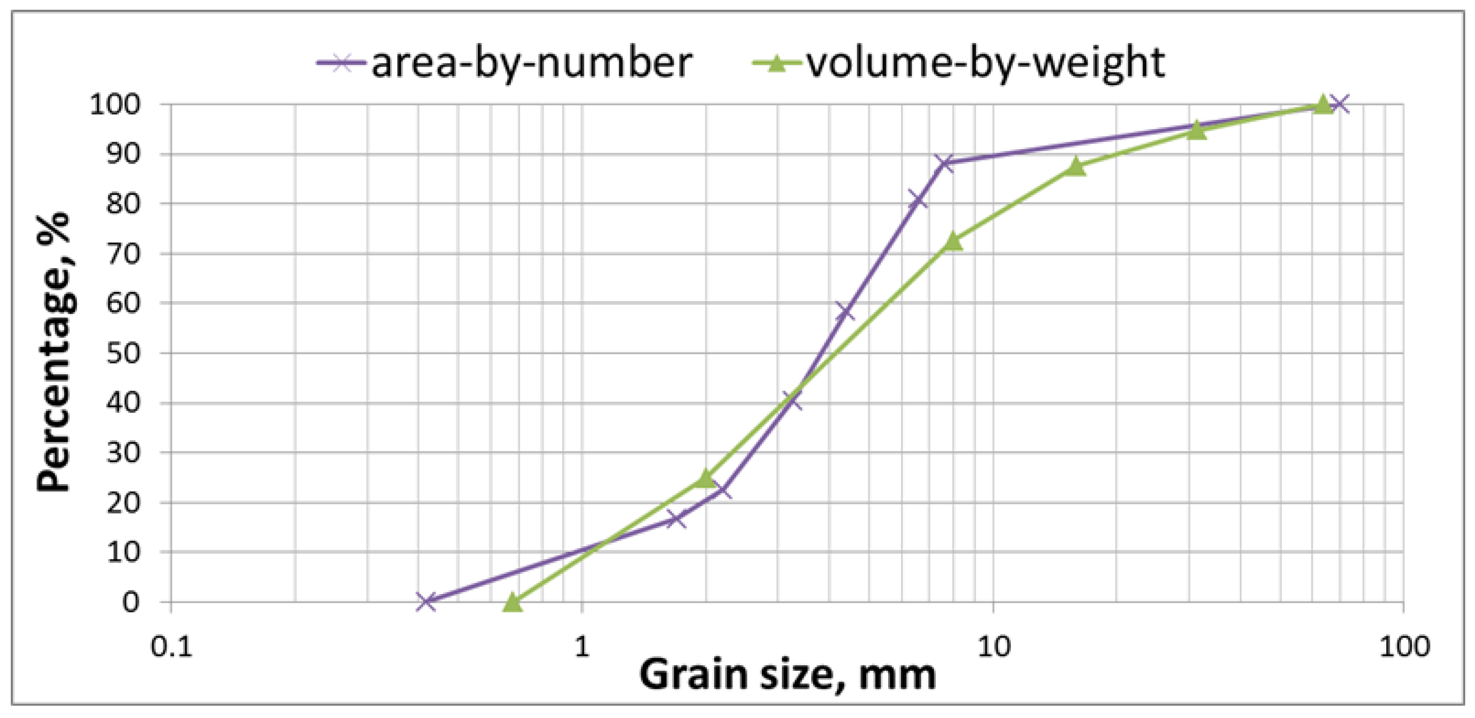
The initial bed material was a sand-gravel mixture (Figure 2), with an initial sand rate of 24.9%. The initial bed material thickness was 21 cm. The grain-size distribution (GSD) of the bed composition was defined by two different methods: volume-by-weight (VbW) and area-by-number (AbN) GSD. The VbW GSD is a more well-known and frequently used description of the material, but needs a physical sample from the bed for the sieve analysis. Since the sampling would have disturbed the content and the compactness of the bed surface, the volume-by-weight method could have only been used at the beginning and at the end of the experiment. On the contrary, the AbN GSD can be defined based on image analysis without disturbing the bed surface. In this study, BASEGRAIN software (ETH, Zurich, Switzerland) was applied, which calculates AbN GSD, based on automatic detection of the grain sizes [20]. Since this method does not disturb the bed surface, it is more suitable to check the bed composition changes at the intermediate equilibrium stages. There are, however, differences in the results of the two methods, so the AbN distribution is not directly comparable to the VbW distribution type [21]. In order to establish a conversion formula, some reference probes (e.g., the initial bed material, see Figure 2) were analysed by both methods. Assuming a linear relationship, a linear function was fitted to the connecting AbN and VbW d50 points. The following formula describes this relation between the AbN and VbW d50 values, which is specific to this study:
where d50,VbW and d50,AbN are the d50 values according to the volume-by-number and area-by-number GSD, respectively. This formula allowed us to compare the experimental and numerical results (the latter will indicate volumetric information).
In addition to the conversion method, there are some further uncertainties regarding the determination of the bed content. The image noise plays an essential role in the results of the image-based method, which can reduce its reliability. When comparing the laboratory experiments and numerical model results, the spatial representivity of the GSD should also be taken into account. The image-based analysis represents an average for a 0.1 m × 0.1 m size square, whereas the numerical model results belong to grid points. On the whole, considering all the above mentioned points, the bed composition comparisons between the laboratory experiment and the numerical model performed in the following sections mean a qualitative assessment rather than a quantitative one.
The VbW and AbN GSD-s of the initial mixture are presented in Figure 2. The mean grain diameter is dm = 8.7 mm, and d50 = 5.2 mm, determined from the VbW GSD.
Besides the bed composition analysis, the flow and bed morphology adjustments were also measured throughout the flume experiments and described in the flowing sections.
For the purpose of flow pattern recognition, vertical velocity profiles were produced with a 3D Acoustic Doppler Velocimeter (ADV) (Nortek A S, Rud, Norway), having 6–12 points per vertical. The acceleration correlation filter method [22] was applied to filter the recorded velocity data. Also, based on the analysis of Kim et al. [23] and Biron et al. [24], the TKE-Method [25] was applied in this study for bed shear stress estimation. Note that considering the uncertainty of the parameter estimation, we focused on characterizing the spatial variability of the bed shear stress instead of the exact quantities.
As for the bed morphology monitoring, the bed geometry was measured at each equilibrium state along the entire flume using a laser scanner device. Furthermore, the sediment discharge at the flume outlet was estimated several times during a run, based on the captured sediment amount by the sediment trap.
The flow measurement, sediment transport and bed morphology analysis procedures and the data processing are detailed in Török et al. [19].
2.2. Assessment of Laboratory Experiments
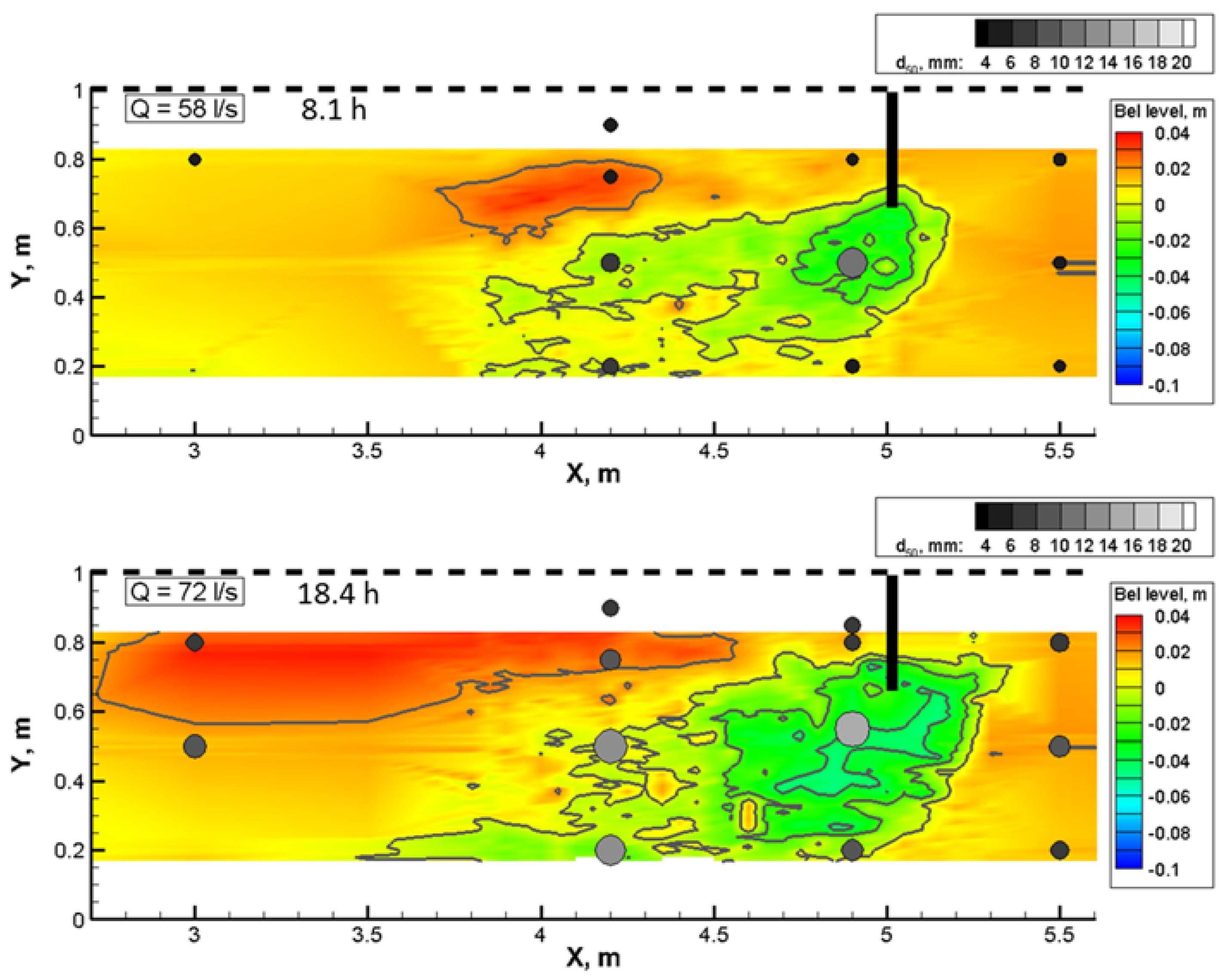
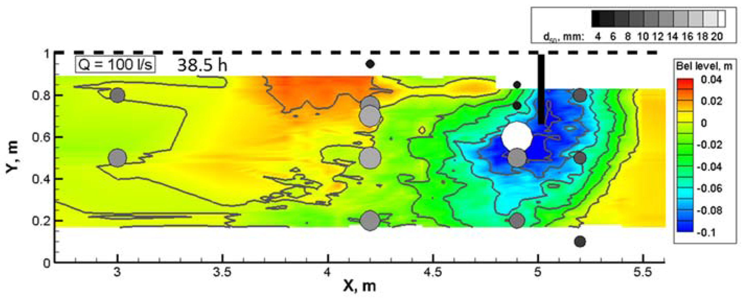
After reaching each equilibrium state, the bed geometry along the entire flume was measured. Figure 3 shows the bed level changes between the equilibrium states. The local AbN d50 values are indicated by circles on the plots.
Based on Figure 3, the local scour hole development at the obstacle edge, and a deposition formation downstream can be investigated. The coloring of the field indicates the bed changes, and the local d50 values could be assessed—the larger and lighter the circle, the coarser the bed material, also shown in Figure 3.
Noticeable is the higher the constant flow discharge, the deeper and wider the score hole. Moreover, the spatial distribution of the d50 indicates bed material coarsening in the erosion zone, which refers to the bed armoring process. The initial d50 = 5.2 mm increased remarkably up to 21 mm until the end of the last run.
At the downstream side of the obstacle, an aggradation process could be observed, which is indicated by the red spot in Figure 3. It can be generally stated that the eroded materials from the tip of the structure were being transported in the downstream direction as long as the sediment transport capacity of the flow is high enough. This phenomenon resulted in a local sediment deposition during the first run, around 1 m downstream of the groin. Because of the higher transport capacity in the second run, the eroded sediments were transported farther. Thus, the deposition form extended until 2.5 m downstream of the groin. In turn, during the third model run, almost the whole sediment deposition was eroded and washed out, which clearly refers to the significantly increased transport capacity. This statement is supported by the analysis of the spatial d50 distribution; Figure 3 shows, that due to the persisting selective erosion process and the higher erosion capability of the flow, the finer fractions are entrained during the last model run, resulting in an increasing d50 along the entire study domain. The areal distribution of the d50 sizes also indicates that the bed material in the recirculation zone became finer than in the main stream. Indeed, the eroded finer fractions from the scour are trapped in the zone.
The scouring and aggregation processes were examined based on the measured bed change time series from the scour hole and the deposition. These points were located at x = 4.98 m; y = 0.59 m (scour hole) and at x = 4.50 m; y = 0.75 m (deposition) inside the monitored area (in the 80 cm close surroundings of the obstacle, in the downstream direction) by bed change sensors. These can be seen in Figure 4.
It can be observed that the scouring process is a much faster process than deposition in the rectangular zone. In Figure 4, the blue and the red lines show the time-series of the deepest point and one from the deposition, respectively. Compared to the last run (18.4 h–38.5 h) it turns out that the scour hole forms in a relatively short time (the equilibrium scour depth developed until the 24th hour) compared to the deposition (the equilibrium deposition height developed until the 30th hour). The scour hole development is, however, somewhat slower in the third run than in the first two cases which likely results from the arriving sediment from upstream, where bed erosion took place.
The bed level changes and bed content data provided the benchmark for the numerical model validation.
3. Numerical Modeling
The flume measurements used for model validation was summarized in Section 2, where the morphological features were also presented. As shown, the bed armoring process and the transport of finer particles were also revealed. Therefore, when selecting the suitable formulas to be used in the numerical model we considered the following: one of the transport models has to be able to describe the coarsening process together with the bed armor development, while the other one has to well estimate the transport of the fine material. For this purpose, the bedload transport equations of Wilcock and Crowe [8] and van Rijn [12] were selected.
The mixture grain-size distribution used in the experiments of Török et al. [19] (Figure 2) and of Wilcock et al. [18] show a good match. In case of the experiments of Wilcock et al. [18], grain size of the initial bed materials was in the range of 4.1–10.5 mm, whereas was 8.7 mm in the measurements of Török et al. The Wilcock and Crowe formula is therefore expected to be capable of describing the gravel/sand bedload transport processes in our experiments. In case of such non-uniform bed material, the interaction between (hiding and exposure) the particles of different sizes play an essential role in the stability of the sediments and can result in bed armoring. The Wilcock and Crowe formula is reported to be capable of predicting the transient conditions of bed armoring, or scouring processes. The preliminary numerical simulations of Török et al. [26] also supported this statement. Note that the equation indicates decreasing particle stability when the sand proportion increases.
The van Rijn bedload formula can be used for particles in the range of 200–2000 μm (i.e., below 2 mm). As such, the formula is not expected to reliably calculate the motion of gravels and the interaction between particles of different sizes and to describe such a process, like bed armoring. However, the model can presumably describe the transport of finer grains.
Both models are well tested and were applied in several numerical modeling studies of riverine sediment transport (e.g., [26,27,28,29,30,31,32,33,34,35]). In this chapter, the implementation and combining of these sediment transport models in a 3D numerical model is presented.
3.1. Applied Numerical Model
The numerical model used in this study [36] solves the 3D Reynolds-averaged Navier-Stokes (RANS) equations with the k-ε turbulence closure (see e.g., [37]) by using a finite-volume method and the SIMPLE algorithm [38] on a 3D non-orthogonal, vertically unstructured grid. The momentum equations are in the complete form, describing the hydrodynamic effects in all directions.
Dirichlet boundary conditions have to be assigned at the inflow boundary. At the outflow boundaries, zero-gradient conditions are used for all variables. The boundary conditions for the RANS equations, at the inflow boundary the water discharge, at the outflow boundary the water level, were set according to the laboratory experiments introduced above (Table 1). In the first cell, on the bed and side walls, the velocity profile is calculated from the well-known logarithmic formula [39]:
where y is the distance from the wall to the center of the cell, U is the boundary aligned velocity, is friction or bed shear velocity, κ is von Karman constant (0.41) and ks is the Nikuradze roughness.
At the water surface, Ux, Uy, P and ε have zero gradient boundary conditions, whereas Uz is set to a certain value and k is equal to zero.
The calculation steps of the numerical model are as follows. Firstly, in a computational time step, the flow solver calculates the pressure and velocity distribution together with the turbulence parameters, TKE (turbulent kinetic energy) and ε (turbulent dissipation). Then, based on the distribution of TKE at the bed, the bed shear stress is derived using the equilibrium formula [25]:
where 𝜏 is the bed shear stress, C1 is a constant (C1 ~ 0.20) and ρ is the water density [23].
The bed composition is then used to calculate the reference, or critical bed shear stress (depends on the given sediment transport formula, discussed later). The volumetric transport rate for each sediment fraction is determined based on the functions of the activated sediment transport formula. Based on the estimated inflowing and transported sediment amount, finally, the bed change can be estimated for each cell. Once the bed geometry is regenerated, a new iteration step starts recalculating the flow field. The iteration steps end if the changed bed form does not result in alteration of the hydrodynamic variables. Then, a new iteration begins for the next time step.
The applied horizontally structured grid can be seen in Figure 5.
In order to ensure the hydrodynamically correct inflow boundary conditions, the computational grid was extended in the upstream direction with a 10 m long section. This virtual section was set to non-erodible. The study domain was discretized with 440 cells in the streamwise direction and 20 cells in the lateral direction, yielding an average horizontal resolution of 0.05 m (Figure 5). Vertically, 9 layers were defined. Local grid refinement was applied in the vicinity of the groin in both horizontal directions to capture the locally high gradients of the flow and sediment transport features. Since only emerged situations were simulated, the grid cells representing the groin were considered to be dry cells.
3.2. Model Setup
The hydrodynamic and sediment transport models were parameterized as described in the following points.
The poorly sorted bed material was discretized with five fractions in the numerical model. The following grain sizes were defined: mm, mm, mm, mm and mm, respectively. Based on the preliminary sieving analysis the following fractions were given: , , , and .
An essential task of the model setup was the determination of the active layer. The concept of the active layer was published, e.g., by Parker et al. [40]. The concept states that the bed can be separated into two layers: the upper is the active, the lower is the substrate layer. The active layer is a given thickness of the surface, which can interact with the transported sediments. Thus, the sediment transport can cause changes (bed level, bed content) only in the active layer, and not in the substrate layer. Accordingly, the bed material can differ in the two layers. The active layer thickness is constant, but the content can change both in time and space. In the case of erosion, the content is replenished from the substrate layer. Otherwise, the deposited sediment also results in some bed content change in the active layer. However, the constant active layer thickness can cause inaccuracy. For example, if the deposition is larger than the active layer, the bed content at the lower part of the deposition will not be equal to the deposited sediment content, but to the bed content of the substrate layer. Such an inaccuracy can lead to further error in the bed change calculation.
In this research, the active layer thickness was determined based mainly on visual observation during the measurements. The initial thickness was set to 0.01 m.
In the flume experiment, no sediment inflow was supplied at the upstream boundary.
3.3. 3D Flow Model Validation
Although the numerical representation of the bed roughness is not straightforward, it is an essential part of the calculation of the sediment transport rate since it directly affects the bed shear stress field. In this regard, a comparative assessment of the bed shear stress values estimated from ADV measurements and the ones calculated by the numerical model was performed. As mentioned before, the ADV measurements were completed at each run after reaching the equilibrium bed geometry and related equilibrium bed material composition. The local bed shear stress values were estimated based on the lowermost point measurements using the TKE Method introduced in Figure 6. In the numerical model, we used two approaches to estimate the bed roughness, according to van Rijn [12] and Wilcock and Kenworthy [7]. The first approach suggests [41], which was elaborated, by van Rijn [42] and the second one suggests [7]. For model validation purposes, the first model variant was used, i.e., a discharge of and an outlet water depth of were defined as boundary conditions at the inlet and outlet sections, respectively. The calculated bed shear stress distributions are presented in Figure 6. The estimated bed shear stress values using the TKE Method are also plotted in the figures as circles.
The estimated local values from ADV measurements are considered as an adequate order of magnitude indicator of the bed shear and accurately show the spatially varying behavior of the parameter. The figures show that the numerical model, where the bed roughness was estimated using the formula, resulted in much better agreement, particularly in the surroundings of the groin. A significant difference cannot be observed, especially taking into account that measurements were not conducted at that exact location. It is also visible that the van Rijn formula results in a major overestimation which, as discussed later on, provokes more intensive erosion in the numerical model than in the experiments.
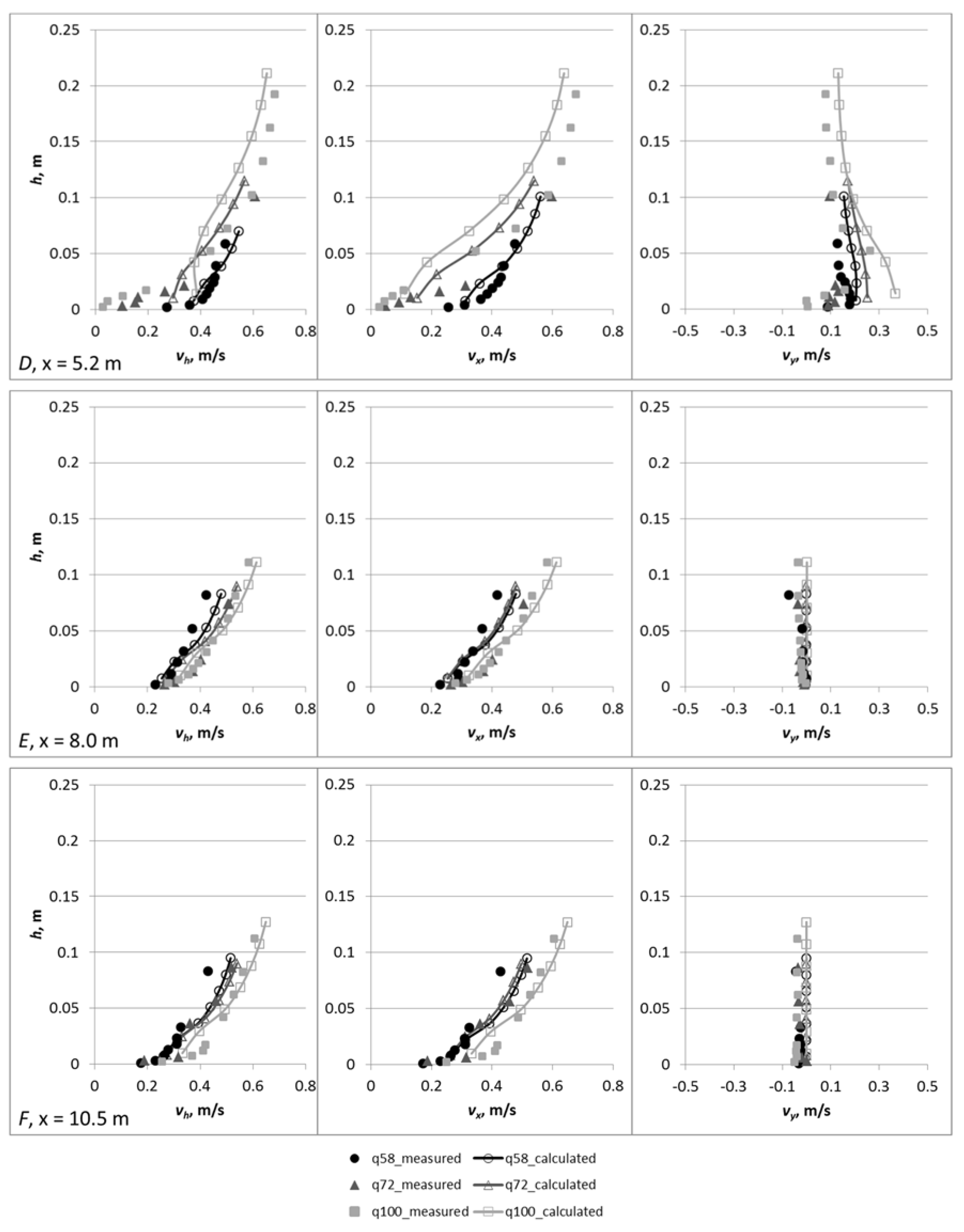
Besides the bed shear stress distribution, time averaged flow velocities were also assessed. Depending on the given water depth, 5–10 points were measured at each vertical based on the flow depth. For model validation purpose, the measured velocity values were compared to the modeled flow velocities. For better understanding not only the horizontal velocity magnitudes were studies, but the velocity vectors were decomposed into streamwise and transverse components (see Figure 7) and the comparative analysis was performed separately, too. Figure 8 shows the vertical velocity distributions both from the measurements (dots) and the numerical model (lines).
In order to avoid the boundary effect caused uncertainties in the numerical model close to the inlet section, the numerical domain was extended in the upstream direction along the length of the flume. Thus, the calculated flow pattern regarding the flume part (x < 11 m) was not disturbed by the boundary effect, including the inlet section (x ≈ 11 m).
Indeed, the agreement between measured and calculated velocities was fairly good already at the most upstream section, at x = 10.5 m. In overall, the streamwise components of the flow velocities were well captured by the numerical model. The vertical distribution does not follow the typically logarithmic profile but rather a combination of two logarithmic functions which can be explained by the complex bed morphology. This behavior can be observed both from the experiments and the numerical calculations. Higher differences are found at locations where the influence of this sort of topographic steering is even stronger, i.e., at the local scour (Figure 8D,E), especially at the highest flow discharge.
As for the transverse velocity components, the deviation from experiments is more substantial. There are some weak transverse flows measured close to inlet and outlet sections (at x = 1 and x = 10.5 m), where the flow pattern would be expected to be more symmetrical. This measured flow pattern appears to have resulted from the transversal non-homogeneous in- and outtake in the laboratory experiments, instead of the effect of the groin. This is therefore not reproduced by the numerical model. On the other hand, the groin and the consequent local scour were influenced by vortex flow, and can be clearly seen at sections x = 5 m and x = 5.2 m. The strongly varying transverse flow vertically is in fact reproduced by the numerical model; however, there are remarkable differences between the measured and calculated values. Higher vertical gradients characterize the secondary flow in the experiments, the reproduction of which is apparently a bottleneck of the numerical model. Indeed, the accurate description of the coherent flow structures around obstacles is a known limitation of the steady RANS modeling (e.g., [43,44,45,46]).
The underestimation of the secondary flow strength can influence the transversal transport of the eroded material which can result in the underestimated mobility of the sediment deposition downstream of the groin. Also, a known limitation of the Reynolds averaged description of the flow field is that the dynamic eddy structure resulting from the vertical shear layer at the obstacle is not reproduced. The increased sediment transport capacity is inherently simulated by the turbulent kinetic energy (see. e.g., [47]) but the temporal variation of this high energy zone is not simulated due to the time-averaged approach. The accurate prediction of the deposition patterns is also an essential goal of this study; however, because of the limitation of the steady RANS modeling, a less mobile deposition pattern can be expected.
3.4. Implementation of Combined Bedload Transport Models
Finally, the numerical implementation of the bedload transport formulas is presented. The computational program [36]—which calculates the hydrodynamics—includes the sediment transport module in a Dynamic Link Library (DLL), which is freely modifiable. The functions of the bedload transport formulas and the criteria—which are discussed later—were implemented by coding them in the DLL file.
The numerical modeling of bedload transport consists of two steps. First, the critical (if van Rijn model is used) [12] or the reference (if the Wilcock and Crowe mode is used) [8] bed shear stress is determined based on the local bed material composition. The critical bed shear stress is defined as the value at which the motion of a given particle size begins [48]. In turn, the reference shear stress is the value at which the dimensionless transport rate () is equal to 0.002, which is a small, but considerable transport rate [49]. Second, the transport rate () is calculated applying the local bed shear stress calculated by the hydrodynamic model. In this study, we propose the spatially and temporally varying combination of the two transport models. A suitable criterion had to be found to decide which formula to use. A preliminary analysis based on the measured spatial and temporal changes of the bed composition showed that a suitable indicator to distinguish between the two approaches of the bedload transport can be the grain size. It was shown, that in zones where the characteristic is lower than the initial , the grain size distribution becomes uniform and the van Rijn formula is expected to be more reliable. This is typically the case outside the region of the scour hole and in the deposition zone downstream of the groin. On the other hand, if the exceeds the initial value, it is the indication of the selective erosion process and the consequent bed armoring, and the Wilcock and Crowe formula will provide better estimates on the bedload transport. In zones where the is around the initial value, a weighted form of the two models is used, in which the weight is calculated according to Equation (4).
Accordingly, the following combination of the two formulas is proposed:
where
Referencing the model setup (Figure 2), the initial VbN was 0.0211 mm.
4. Results and Discussion
The results of the morphodynamic simulations were assessed through the measured versus the calculated equilibrium bed geometry and the corresponding local mean grain size of the bed material. All the three runs were analyzed at Q1 = 58 L/s, Q2 = 72 L/s and Q3 = 100 L/s. Numerical simulations were performed applying the (i) van Rijn bedload transport formula; (ii) Wilcock and Crowe bedload transport formula and (iii) the combined approach. The measured bed geometry after reaching equilibrium conditions at Q1 = 58 L/s indicates the formation of a scour hole at the tip of the groin with a depth of 0.03 m (Figure 9).
The eroded material is partly transported in the downstream direction, and partly captured by the recirculation zone. This leads to the formation of a local deposition zone with a maximum height of 0.02 m. Using the van Rijn formula in the numerical model, a significant overestimation of the bed changes can be observed. The highest point in the deposition zone is around 0.10 m, whereas the deepest point in the scour hole is around 0.14 m. This result clearly confirms that the van Rijn formula overestimates the mobility of the finer particles in the case of a gravel-sand mixture (Figure 9-i). On the other hand, the application of the Wilcock and Crowe formula results in a more realistic bed changes pattern (Figure 9-ii). The depth and the shape of the scour hole are fairly well estimated; however, the size of the deposition zone is considerably larger in the simulations. The location and extension of the sediment deposition is somewhat better predicted with the combined transport formula (Figure 9-iii) as the height of the bar developed in the flume centerline is lower than the one resulting from the Wilcock and Crowe formula. However, this approach still shows overestimation of the deposition pattern. This might be the result of the above-mentioned limitations of the applied 3D RANS flow model.
The spatial distribution of the measured d50 values (circles in Figure 10) indicates an overall coarsening of the bed material after the first run.
It can, however, be observed that the coarsening is stronger in the narrowest section of the flume. In this zone, the original 5.2 mm d50 increases to 12 mm, whereas in the upstream section and in the recirculation zone, the d50 is around the initial diameter. The numerical simulations using the van Rijn formula show unrealistic local coarsening around the groin, enhancing the limitation of this approach when inhomogeneous bed material is present (Figure 10-i). The Wilcock and Crowe formula shows the similar behavior of the d50 pattern along the flume with respect to the measured ones. The selective erosion of the finer particles, i.e., the coarsening in the main stream is well reproduced; however, the coarsest grain size in the scour hole indicates larger grains in the simulations (Figure 10-ii). It has to be noted that the measured (image-based) analysis represents an averaged d50 for a ~0.1 m × 0.1 m size square, whereas the numerical model results belong to the given grid points. The application of the combined formula leads to a very similar pattern of d50 than in the previous model variant. The selective erosion in this case, however, appears along the whole downstream section where the van Rijn model is activated with higher weight in the bedload transport model.
Figure 11 introduces the simulation results for the flow discharge of Q = 72 L/s. As Figure 11 shows, the higher discharge implied more intensive bed changes. The deposition zone shifted closer to the right flume wall and extended mainly in the downstream direction. The elevation of the highest point increased a few cm during this run. On the contrary, the scour hole tended to deepen further and extended to the upstream direction.
As mentioned above, the van Rijn model calculated extremely high morphological changes and so the simulations diverged (results from those simulations are not shown). The elevations of the highest deposition point and the lower scour point, estimated by the Wilcock and Crowe and the combined model, are overestimated in both cases. Neither of the models reproduced the extension of the scour hole towards the upstream direction. The major difference between the Wilcock and Crowe and the combined models is that the combined one indicates higher transport capacity in the main stream, and consequently less deposition can be observed in that version. The d50 distribution of the Wilcock and Crowe model also indicates that the eroded particles were deposited immediately after the erosion zone (Figure 12-ii). Nevertheless, the combined model seems to result in less stable particles in the main stream and so indicates higher d50 values downstream of x = 3.5 m (Figure 12-ii). Thus, the combined model barely calculates deposition in the main stream (Figure 11-iii). The combined model overall shows better agreement with the measurements.
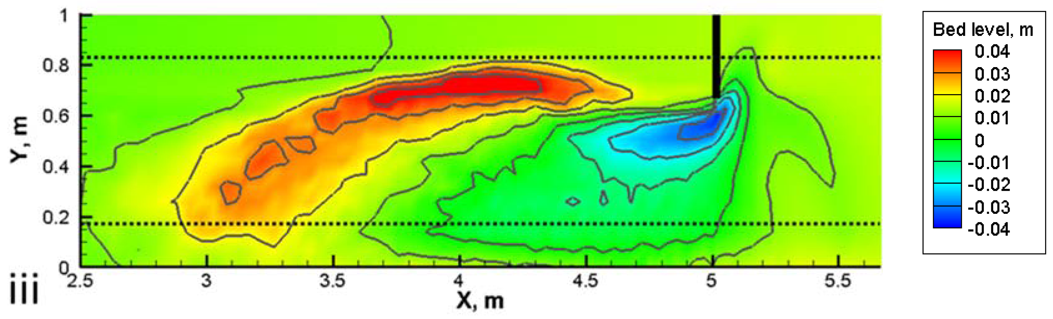
The measured equilibrium bed levels after the last run (Figure 13) show that the local deposition formed during the previous two runs stopped growing; moreover, a part of it was eroded.
As it could be observed in the laboratory experiment, a significant amount of the sediments was exported from the flume suddenly at the highest discharge, while the rest, as a dune formation, tended to shift much slower towards the outlet direction [19]. This deposition zone reached a stable state before the outlet section. It can be observed that the lowest point in the scour hole deepened by 4 cm. The highest parts of the deposition zone also decreased, showing a total deposition height of 1.5 cm compared to the initial bed level.
The calculated final bed levels can be seen in Figure 13-ii and in Figure 13-iii. Similar to the experiments, the further deepening at the tip of the groin is visible. Similar to the previous cases, the estimated level of the deepest point was acceptable; the difference was less than 1.5 cm. Although the Wilcock and Crowe model was not able to reproduce the erosion in the upstream from the groin, a major difference can be noticed at the downstream part of the scour hole. In accordance with the previously experienced behavior of the models, the Wilcock and Crowe model overestimates the stability of the finer eroded sediments, indicating a fairly stable position. Accordingly, not only local deposition occurs, but the surrounding averaged bed level also increased. It is also remarkable that a significantly higher (~2 cm) deposition zone formed. In contrast to the laboratory measurement, no dune formation could be detected at the outlet section in Figure 13-ii and in Figure 13-iii. However, the deposition zones have two peaks. This suggests a similar phenomenon as in the laboratory case: a part of the dune formation tended to shift downstream and separated. Although the combined approach was not able to reproduce the dune formation at the outlet section, the separation of the dunes and the shifting of the lower dune were modeled more reliably.
Table 2 and Table 3 show data on the volumes of the deposition forms. Table 2 shows the ratio of the calculated and measured dune volumes for each model run. A value of 1 would indicate a perfect match to the measured volume.
Table 2 shows that the combined approach yields a better agreement with the measured data. Especially in the second model run, the rate of 1.1 means quite a reliable calculation of the deposition volume. However, in the first and last runs, the differences between the two models are not significant, but the combined approach resulted in better estimated volumes in both cases. In the case of the last model run, the ratio of the shifted dune and the total deposition volumes were also calculated with respect to the measurement, the Wilcock and Crowe and the combined approach model runs. These ratio values can be seen in Table 3. The values still show considerable disagreement in the case of both models. However, compared with the rate of the Wilcock and Crowe to the rate of combined model, the combined approach more accurately estimates the detachment of the shifting dune. This difference is the effect of the involvement of the van Rijn formula.
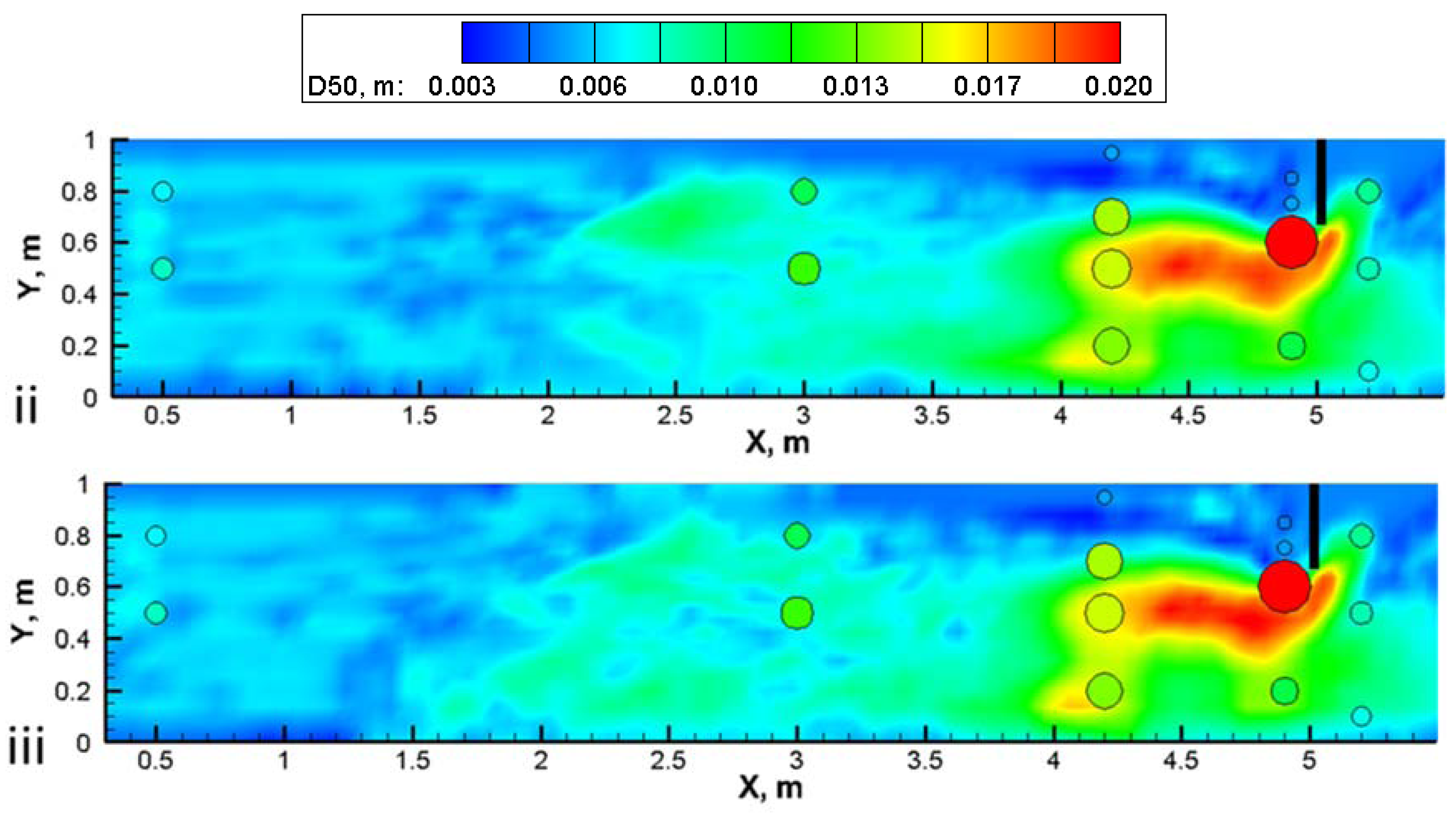
The d50 distribution calculated by the Wilcock and Crowe model refers to the resuspension of the fine particles, which indicates the disappearance of fine materials along the downstream half of the flume.
The agreement between the calculated (field) by Wilcock and Crowe and measured (dots) d50 distribution of the bed material suggests the applicability of the Wilcock and Crowe model. The calculated distribution not only reproduces the spatial patterns but also shows an acceptable quantitative match (Figure 14-ii).
Since there was no considerable difference between the two calculated d50 distribution fields (Figure 14-ii,iii), the d50 distribution calculated by the combined approach has the same precision as the Wilcock and Crowe formula. However, there is no measured point between x = 1.5–3 m, where the deposition dune stopped moving forward during the combined approach calculation. Figure 14-iii indicates some coarsening (x > 1.5 m, green spots, d50 > 0.01 m) around this region. A possible reason for this phenomenon can be the above detailed incorrect effect of the constant active layer. Accordingly, the lower part of the deposition is taken into account by the numerical model as being coarser than it is. Thus, a more stable deposition is assumed, leading to the stoppage of the dune.
At the highest discharge, in both model variants, the deposition zone shifted towards the downstream direction, but no lateral displacement was simulated as occurred in the experiments. Therefore, the easily erodible fine particles did not enter the main stream. According to Figure 8B,C, the flow model underestimates the cross-directional velocity values at the deposition zone. Thus, the eroded sediments tend to transfer to the right wall and settle. This can be another explanation for the underestimation of the out-washed sediment amount. Moreover, this can explain why the numerical models estimate larger deposition on the right side of the flume. This experience also draws attention to the importance of the further development of the 3D numerical flow modeling.
Summarizing the above, the combined model reproduces fairly well the bed changes compared to the measurements, even better than the Wilcock and Crowe formula. The significant difference between the results of the Wilcock and Crowe and the combined approach appears at the lower section again (in the deposition zone, around x = 1.5–4 m). The combined model calculated higher sediment transport of the eroded sediments than the Wilcock and Crowe formula. The local deposition at the outlet section seems to be developing, which underlines the benefit of the combined model, estimating higher transport capacity for the fine fractions compared to the Wilcock and Crowe model. Indeed, the low transport rate of the sand particles estimated by the Wilcock and Crowe formula can be corrected by using a more suitable formula in those zones. The application of different sediment transport formulas in these regions can also be justified with the findings of Jaggi [50], who used the particle Froude number (dimensionless bed shear stress) to distinguish between sediment transport modes:
Based on this classification, weak transport characterizes the deposition zone (where is around 0.01), while mobile armoring characterizes the erosion zone at the tip of the groin (where is around 0.08), indeed calling for different approaches for the transport modeling.
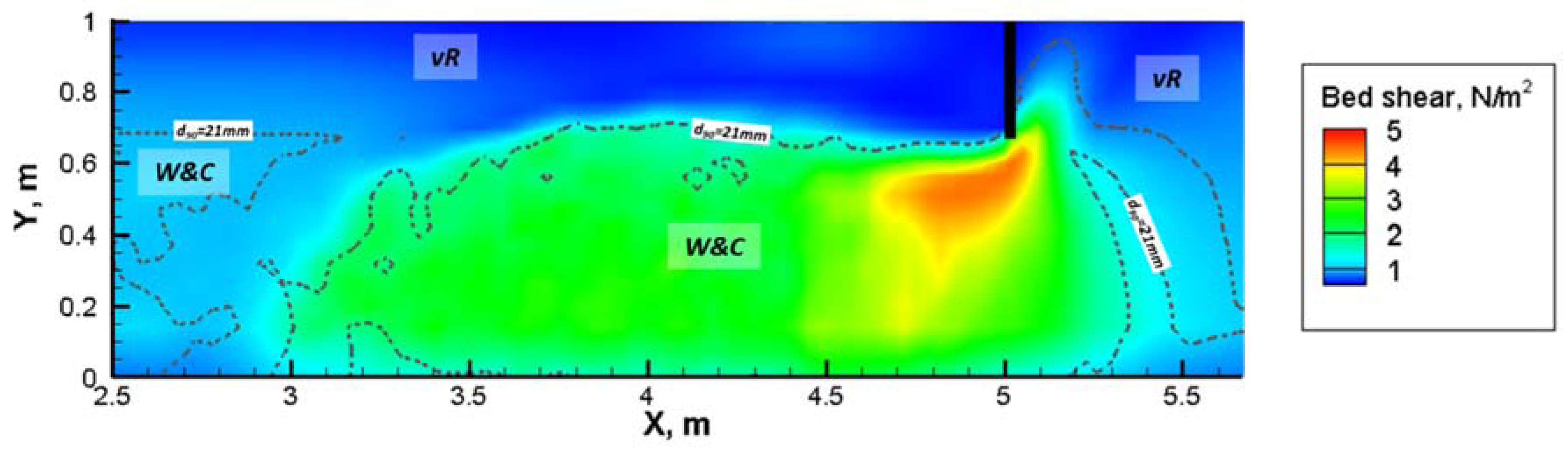
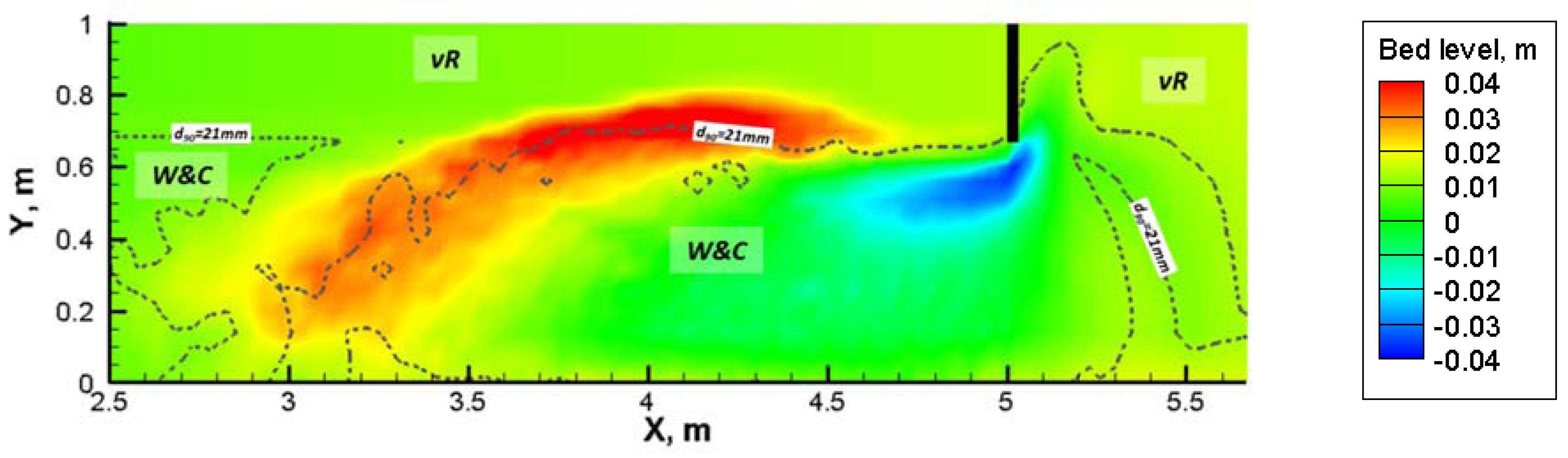
Finally, the spatial behavior of the combined sediment transport model is assessed. Figure 15 and Figure 16 show the equilibrium bed levels and bed shear stress distribution calculated by the combined approach, at the lowermost discharge. The dotted lines refer to the d90 = 0.021 m isolines, which bound the regions where the Wilcock and Crowe formula is applied. The off-line areas show the regions where the van Rijn model calculates the sediment transport.
A larger part of the deposition zone (red spot, behind the groin in Figure 15, blue spot in Figure 16) was formed primarily from the finer fractions and belongs to the van Rijn formula. Although the van Rijn model estimates much higher mobility for the smaller particles, the transport capacity is still too low () to transport even the smaller grains (see Section 3.4). On the other side of the d90 = 0.021 m isoline, the bed material is coarser and the Wilcock and Crowe formula is activated. In this zone, the transport capacity of the flow is higher (), but the estimated higher stability of the grains leads to a resistant bed formation. Thus, the combined application of the two formulas with the above presented conditions (Equations (4) and (5)) results in the described equlibrium bed formation. The formed dune ridge of the deposition zone (red spot in Figure 15) designates the places where the morphological conditions () do not result in any substantial sediment transport according to both formula.
5. Conclusions
In this paper, we introduced a novel approach to simulate sediment transport and related morphological changes in complex hydro-morphological situations, implementing and combining the Wilcock and Crowe [8] and the van Rijn [12] bedload transport models in a 3D numerical hydrodynamic model. The reason for this development was the fact that most of the empirical sediment transport formulas are not generally applicable for spatially and temporally strongly varying flow and sediment conditions, such as the development of local scour together with the transport of fine material. Through a comparative analysis with flume experiments of mixed size bed material, the capabilities of the numerical model were tested coupling the two, significantly different sediment transport formulas. The developed numerical tool distinguishes spatially and temporally between the two formulas, based on an indicator grain size and uses the Wilcock and Crowe model where the mixed sediment dominates and the van Rijn model where sand dominates. The improved numerical model gives better estimation of the morphological changes than the separate application of the models. The considerable differences compared to the single application of the Wilcock and Crowe model occurs mainly with respect to the calculation of the motion and deposition of the eroded sediments. The combined approach resulted in a better match to the measurements, which is enough to underline the potential of development. However, the presented combination method should not be considered as a generally validated sediment transport model, but as a demonstration of the benefit of the coupled application of sediment transport models.
It is important to note that it seems to be quite a challenging task to provide reliable experimental data for model validation. In this study, a thorough analysis of the flow, sediment transport and morphological changes was performed; however, the temporal changes could hardly be detected as opposed to the equilibrium conditions. The utilization of surrogate techniques for bed load transport measurements might be a suitable way to reveal the temporal behavior of the sediment transport. For instance, acoustic measurements using Acoustic Doppler Current Profiler ADCP to track the bed movement based on bottom tracking [51] could be applied. Also, the continuous measurement of the bed morphology could support the numerical model validation, for which ultrasonic [52] and coupled ultrasonic and laser techniques [53] were recently tested.
The future goal is obviously to apply the developed numerical tool to field-scale problems. An issue to be further investigated is, however, the scale-effect, which is likely presented when performing laboratory analysis of sediment transport. Therefore, a proper continuation of the present study would be to validate the model on the prototype scale and to reveal the major differences between the two scales in terms of the main features of the sediment transport. Indeed, the reliable morphodynamic modeling of rivers with complex flow and sediment transport characteristics is of major interest since economic, environmental and social impacts are directly connected to river morphology.
Acknowledgments
The support of the Norway Grant Mobility program (Grant Agreement number: EGT/156/M2-0007) is acknowledged, which made possible the personal discussions among the authors. We acknowledge the funding of the second author from the János Bolyai fellowship of the Hungarian Academy of Sciences. This work was partly supported by MTA TKI of the Hungarian Academy of Sciences. We also would like to thank Nils Reidar Olsen for the valuable advice regarding the numerical model implementation.
Author Contributions
Gergely T. Török developed the combined sediment transport model, performed the numerical model tests and prepared the draft version of this paper. Sándor Baranya and Nils Rüther continuously contributed to the model development stage with theoretical considerations and practical guidance, and to the preparation of the paper with proof reading and corrections.
Conflicts of Interest
The authors declare no conflict of interest.
References
- Parker, G. Transport of Gravel and Sediment Mixtures. In Sedimentation Engineering: Processes, Measurements, Modeling, and Practice; García, M., Ed.; ASCE: Reston, VA, USA, 2008; pp. 165–251. [Google Scholar]
- Meyer-Peter, E.; Müller, R. Formulas for Bed-Load Transport. In Proceedings of the Second Congress IAHR, Stockholm, Sweden, 7–9 June 1948.
- Einstein, H.A. The Bed-Load Function for Sediment Transportation in Open Channel Flows; Technical Bulletin; U.S. Department of Agriculture: Washington, DC, USA, 1950; p. 71.
- Ashida, K.; Michiue, M. Study on hydraulic resistance and bedload transport rate in alluvial streams. Trans. Jpn. Soc. Civ. Eng. 1972, 206, 59–69. [Google Scholar] [CrossRef]
- Parker, G.; Klingeman, P.C.; Mclean, D.G. Bedload and Size Distribution in Paved Gravel-Bed Streams. J. Hydraul. Div. 1982, 108, 544–571. [Google Scholar]
- Parker, G. Surface-Based Bedload Transport Relation for Gravel Rivers. J. Hydraul. Res. 1990, 28, 417–436. [Google Scholar] [CrossRef]
- Wilcock, P.R.; Kenworthy, S.T. A two-fraction model for the transport of sand/gravel mixtures. Water Resour. Res. 2002, 38, 1194–1205. [Google Scholar] [CrossRef]
- Wilcock, P.R.; Crowe, J.C. Surface-based transport model for mixed-size sediment. J. Hydraul. Eng. 2003, 129, 120–128. [Google Scholar] [CrossRef]
- Wu, W.; Wang, S.S.Y.; Jia, Y. Nonuniform sediment transport in alluvial rivers. J. Hydraul. Res. 2000, 38, 427–434. [Google Scholar] [CrossRef]
- Powell, D.M.; Reid, I.; Laronne, J.B. Evolution of bed load grain size distribution with increasing flow strength and the effect of flow duration on the caliber of bed load sediment yield in ephemeral gravel bed rivers. Water Resour. Res. 2001, 37, 1463–1474. [Google Scholar] [CrossRef]
- Yang, C.T.; Wan, S. Comparison of Selected Bed-Material Load Formulas. J. Hydraul. Res. 1991, 117, 973–989. [Google Scholar] [CrossRef]
- Van Rijn, L.C. Sediment Transport, Part I, Bed Load Transport. J. Hydraul. Eng. 1984, 110, 1431–1456. [Google Scholar] [CrossRef]
- Fernandez Luque, R. Erosion and Transport of Bed-load Sediment. Bachelor’s Thesis, Delft Technical University, Delft, The Netherlands, 1974. [Google Scholar]
- Fernandez Luque, R.; van Beek, R. Erosion and Transport of Bed-load Sediment. J. Hydraul. Res. 1976, 14, 127–144. [Google Scholar] [CrossRef]
- Guy, H.P.; Simons, D.B.; Richardson, E.V. Summary of Alluvial Channel Data from Flume Experiments, 1956–1961; Geological Survey Professional Paper; USGS: Washington, DC, USA, 1966; 104p.
- Stein, R.A. Laboratory Studies of Total Load and Apparent Bed Load. J. Geophys. Res. 1965, 70, 1831–1842. [Google Scholar] [CrossRef]
- Delft Hydraulics Laboratory. Verification of Flume Tests and Accuracy of Flow Parameters; Note R 657-VI; Delft Hydraulics Laboratory: Delft, The Netherlands, 1979. [Google Scholar]
- Wilcock, P.R.; Kenworthy, S.T.; Crowe, J.C. Experimental study of the transport of mixed sand and gravel. Water Resour. Res. 2001, 37, 3349–3358. [Google Scholar] [CrossRef]
- Török, G.T.; Baranya, S.; Rüther, N.; Spiller, S. Laboratory analysis of armor layer development in a local scour around a groin. In Proceedings of the International Conference on Fluvial Hydraulics River Flow, Lausanne EPFL, Lausanne, Switzerland, 3–5 September 2014.
- Detert, M.; Weitbrecht, V. User guide to gravelometric image analysis by BASEGRAIN. In Advances in Science and Research; Fukuoka, S., Nakagawa, H., Sumi, T., Zhang, H., Eds.; Taylor & Francis Group: London, UK, 2013. [Google Scholar]
- Strom, K.B.; Kuhns, R.D.; Lucas, H.J. Comparison of Automated Image-Based Grain Sizing to Standard Pebble-Count Methods. J. Hydraul. Eng. 2010, 136, 461–473. [Google Scholar] [CrossRef]
- Cea, L.; Puertas, J.; Pena, L. Velocity measurements on highly turbulent free surface flow using ADV. Exp. Fluids 2007, 42, 333–348. [Google Scholar] [CrossRef]
- Kim, S.C.; Friedrichs, C.T.; Maa, J.P.Y.; Wright, L.D. Estimating bottom stress in tidal boundary layer from Acoustic Doppler velocimeter data. J. Hydraul. Eng. 2000, 126, 399–406. [Google Scholar] [CrossRef]
- Biron, P.M.; Robson, C.; Lapointe, M.F.; Gaskin, S.J. Comparing different methods of bed shear stress estimates in simple and complex flow fields. Earth Surf. Process. Landf. 2004, 29, 1403–1415. [Google Scholar] [CrossRef]
- Soulsby, R.L.; Dyer, K.R. The form of the near-bed velocity profile in a tidally accelerating flow. J. Geophys. Res. Oceans 1981, 86, 8067–8074. [Google Scholar] [CrossRef]
- Török, G.T.; Baranya, S.; Rüther, N. Three-dimensional numerical modeling of non-uniform sediment transport and bed armoring process. In Proceedings of the 18th Congress of the Asia & Pacific Division of the IAHR 2012, Jeju, Korea, 19–23 August 2012. Paper 0816.
- Fischer-Antze, T.; Rüther, N.; Olsen, N.R.B.; Gutknecht, D. 3D modeling of non-uniform sediment transport in a channel bend with unsteady flow. J. Hydraul. Res. 2009, 47, 670–675. [Google Scholar] [CrossRef]
- Gaeuman, D.; Andrews, E.D.; Krause, A.; Smith, W. Predicting fractional bed load transport rates: Application of the Wilcock-Crowe equations to a regulated gravel bed river. Water Resour. Res. 2009, 45, W06409. [Google Scholar] [CrossRef]
- Janssen, S.R. A Part of Transport: Testing Sediment Models under Partial Transport Conditions. Master’s Thesis, University of Twente, Enschede, The Netherlands, 2010. [Google Scholar]
- Rüther, N.; Olsen, N.R.B. Modelling free-forming meander evolution in a laboratory channel using three-dimensional computational fluid dynamics. Geomorphology 2007, 89, 308–319. [Google Scholar] [CrossRef]
- Rüther, N.; Olsen, N.R.B. 3D modeling of transient bed deformation in a sine-generated laboratory channel with two different width to depth ratios. In Proceedings of the International Conference on Fluvial Hydraulics, Lisbon, Portugal, 6–8 September 2006.
- Rüther, N.; Olsen, N.R.B. Three-dimensional modeling of sediment transport in a narrow 90° channel bend. J. Hydraul. Eng. 2005, 131, 917–920. [Google Scholar] [CrossRef]
- Olsen, N.R.B.; Melaaen, M.C. Three-dimensional calculation of scour around cylinders. J. Hydraul. Eng. 1993, 119, 1048–1054. [Google Scholar] [CrossRef]
- Bihs, H.; Olsen, N.R.B. Numerical Modeling of Abutment Scour with the Focus on the Incipient Motion on Sloping Beds. J. Hydraul. Eng. 2011, 137, 1287–1292. [Google Scholar] [CrossRef]
- Zinke, P.; Olsen, N.R.B.; Bogen, J. Three-dimensional numerical modelling of levee depositions in a Scandinavian freshwater delta. Geomorphology 2011, 129, 320–333. [Google Scholar] [CrossRef]
- Olsen, N.R.B. A Three-Dimensional Numerical Model for Simulation of Sediment Movements in Water Intakes with Moving Option; User’s Manual 2002; Department of Hydraulic and Environmental Engineering, The Norwegian University of Science and Technology: Trondheim, Norway, 2002. [Google Scholar]
- Pope, S.B. Turbulent Flows; Cambridge University Press: Cambridge, UK, 2000. [Google Scholar]
- Patankar, S.V. Numerical Heat Transfer and Fluid Flow; McGraw-Hill Book Company: New York, NY, USA, 1980. [Google Scholar]
- Schlichting, H. Boundary Layer Theory; McGraw-Hill: New York, NY, USA, 1979. [Google Scholar]
- Parker, G.; Paola, C.; Leclair, S. Probabilistic Exner Sediment Continuity Equation for Mixtures with No Active Layer. J. Hydraul. Eng. 2000, 126, 818–826. [Google Scholar] [CrossRef]
- Villaret, C.; Van, L.A.; Huybrechts, N.; Van Pham Bang, D.; Boucher, O. Consolidation effects on morphodynamics modelling: Application to the Gironde estuary. La Houille Blanch. 2010, 6, 15–24. [Google Scholar] [CrossRef]
- Van Rijn, L.C. Equivalent roughness of alluvial bed. J. Hydraul. Eng. 1982, 108, 1215–1218. [Google Scholar]
- Koken, M.; Constantinescu, G. An investigation of the flow and scour mechanisms around isolated spur dikes in a shallow open channel: 2. Conditions corresponding to the final stages of the erosion and deposition process. Water Resour. Res. 2008, 44, W08407. [Google Scholar] [CrossRef]
- Catalano, P.; Wang, M.; Iaccarino, G.; Moin, P. Numerical simulation of the flow around a circular cylinder at high Reynolds numbers. Int. J. Heat Fluid Flow 2003, 24, 463–469. [Google Scholar] [CrossRef]
- Roulund, R.; Sumer, B.M.; Fredsøe, J.; Michelsen, J. Numerical and experimental investigation of flow and scour around a circular pile. J. Fluid Mech. 2005, 534, 351–401. [Google Scholar] [CrossRef]
- Baranya, S.; Olsen, N.R.B.; Stoesser, T.; Sturm, T. Three-dimensional RANS modeling of flow around circular piers using nested grids. Eng. Appl. Comput. Fluid Mech. 2012, 6, 648–662. [Google Scholar] [CrossRef]
- Baranya, S.; Józsa, J. Investigation of flow around a groin with a 3D numerical model, II. In Proceedings of the Ph.D. CivilExpo Symposium, Budapest, Hungary, 29–31 January 2004; pp. 12–19.
- Shields, A.F. Application of Similarity Principles and Turbulence Research to Bed-Load Movement; California Institute of Technology: Pasadena, CA, USA, 1936; Volume 26, pp. 5–24. [Google Scholar]
- Parker, G.; Dhamotharan, S.; Stefan, H. Model experiments on mobile, paved gravel bed streams. Water Resour. Res. 1982, 18, 1395–1408. [Google Scholar] [CrossRef]
- Jaeggi, M.N.R. Effect of Engineering Solutions on Sediment Transport. In Dynamics of Gravel-Bed Rivers; Billi, P., Hey, R.D., Thorne, C.R., Tacconi, P., Eds.; John Wiley & Sons Ltd.: Hoboken, NJ, USA, 1992. [Google Scholar]
- Ramooz, R.; Rennie, C.D. Laboratory measurement of bedload with an ADCP. In Bedload-Surrogate Monitoring Technologies; U.S. Geological Survey Scientific Investigations Report 2010-5091; Gray, J.R., Laronne, J.B., Marr, J.D.G., Eds.; USGS: Reston, VA, USA, 2010. [Google Scholar]
- Muste, M.; Baranya, S.; Tsubaki, R.; Kim, D.; Ho, H.; Tsai, H.; Law, D. Acoustic mapping velocimetry. Water Resour. Res. 2016, 52, 4132–4150. [Google Scholar] [CrossRef]
- Visconti, F.; Stefanon, L.; Camporeale, C.; Susin, F.; Ridolfi, L.; Lanzoni, S. Bed evolution measurement with flowing water in morphodynamics experiments. Earth Surf. Process. Landf. 2012, 37, 818–827. [Google Scholar] [CrossRef]
Figure 1.
The interpretation of the local coordinate system [19].
Figure 1.
The interpretation of the local coordinate system [19].

Figure 2.
The initial area-by-number (purple) and volume-by-number (green) grain-size distribution of the bed material.
Figure 2.
The initial area-by-number (purple) and volume-by-number (green) grain-size distribution of the bed material.

Figure 3.
Contour plots: bed changes distribution after each experiment. Circles: local VbW d50 (volume-by-weight) values of the bed surface (size and tone indicate size).
Figure 3.
Contour plots: bed changes distribution after each experiment. Circles: local VbW d50 (volume-by-weight) values of the bed surface (size and tone indicate size).


Figure 4.
The bed change time series in the deposition zone (red line and dots) and in the scour hole (blue line and dots). The discharge time series is also visualized by the black solid line.
Figure 4.
The bed change time series in the deposition zone (red line and dots) and in the scour hole (blue line and dots). The discharge time series is also visualized by the black solid line.
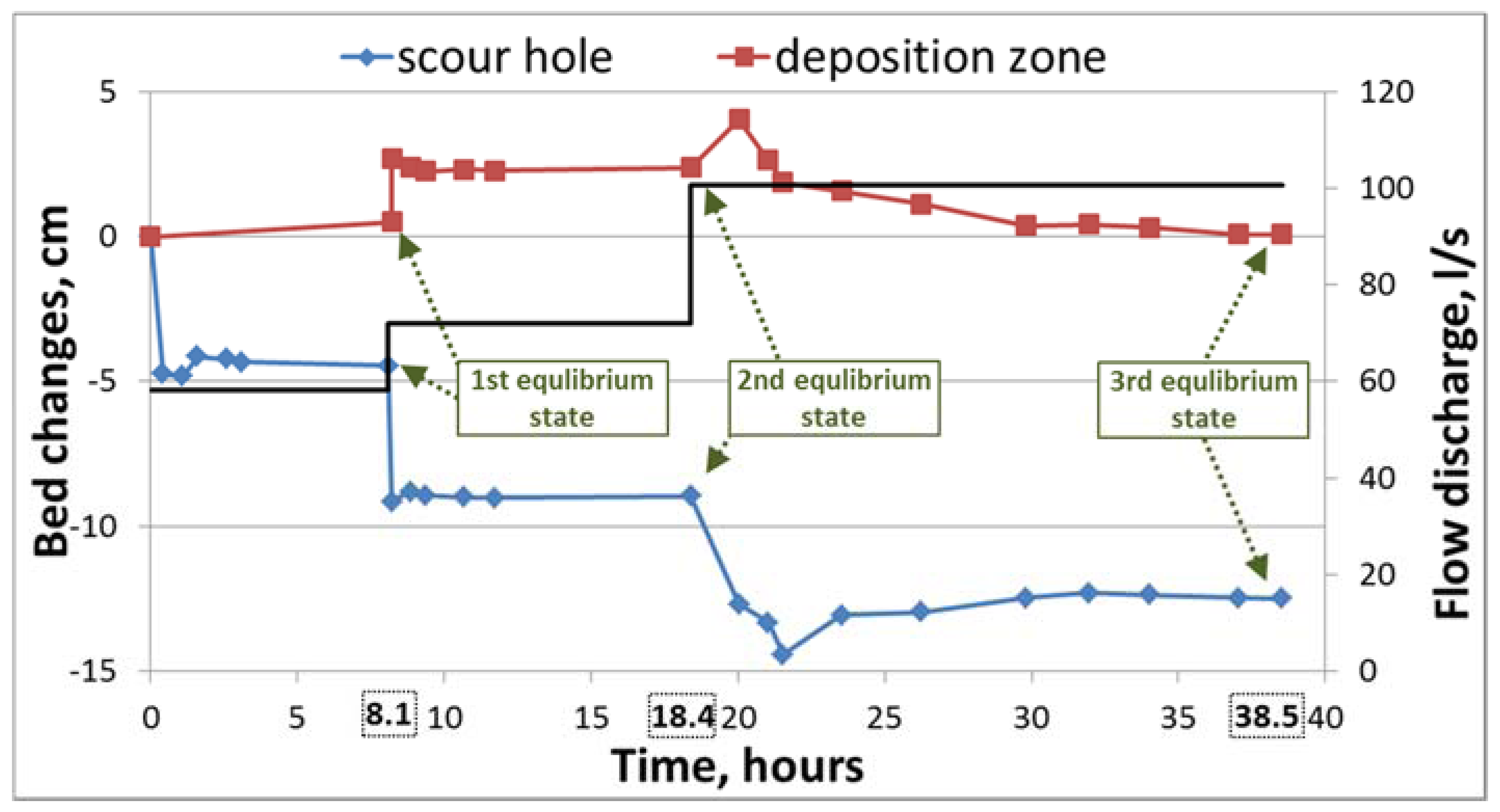
Figure 5.
Sketch of the computation grid.
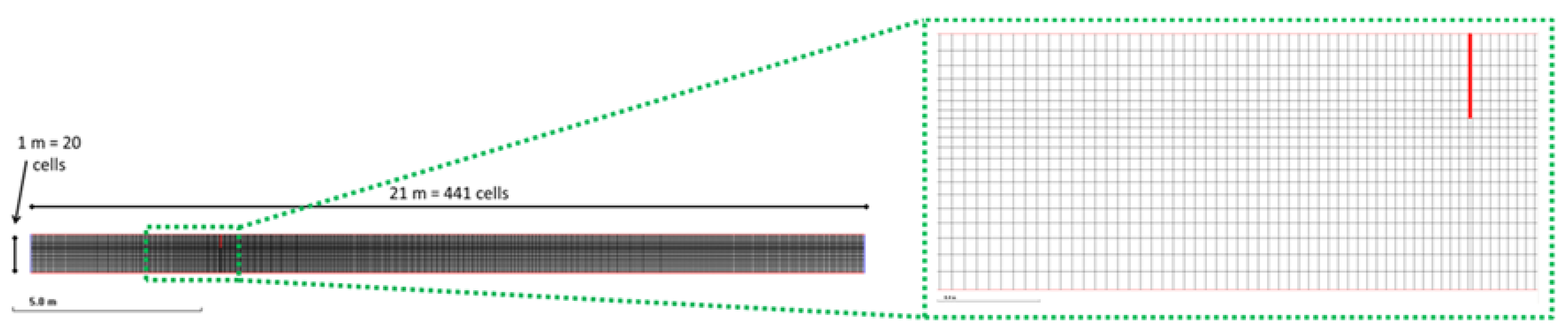
Figure 6.
Calculated bed shear stress distribution by the numerical 3D model. Above: ; below: . Circles refer to the estimated shear values from the ADV (Acoustic Doppler Velocimeter) measurements.
Figure 6.
Calculated bed shear stress distribution by the numerical 3D model. Above: ; below: . Circles refer to the estimated shear values from the ADV (Acoustic Doppler Velocimeter) measurements.
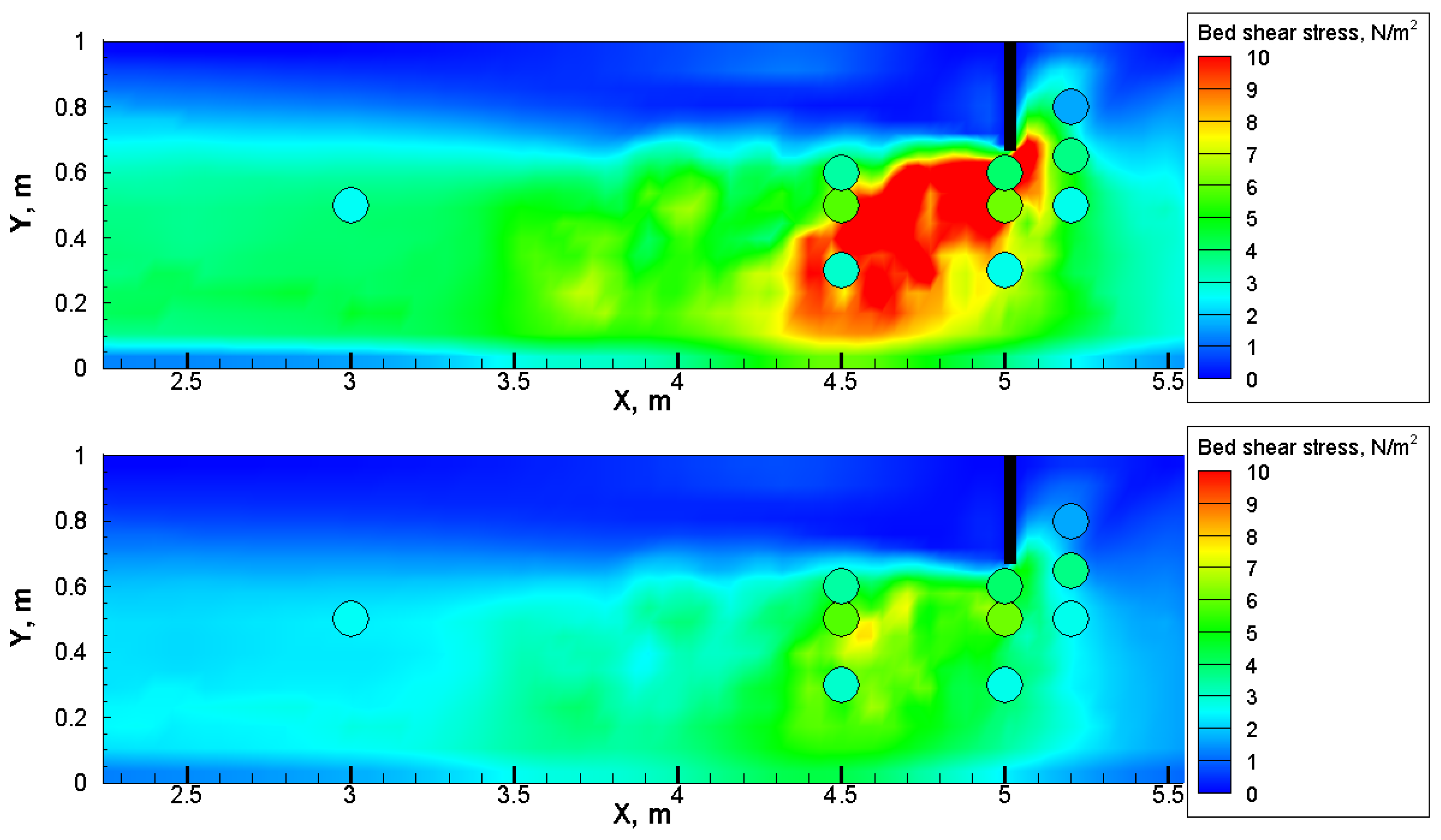
Figure 7.
The interpretation of the signs of the velocity vectors.
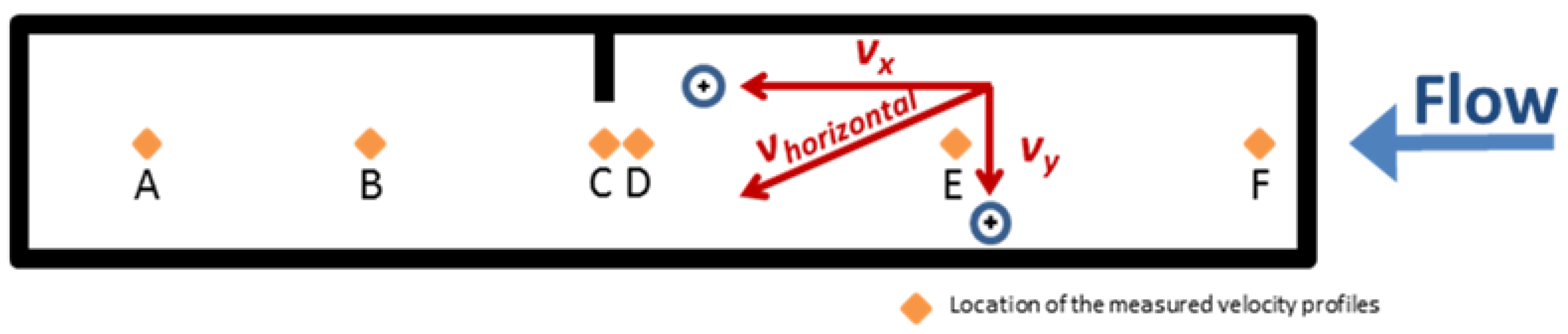
Figure 8.
Calculated and measured vhozitontal (first column), vx (second column) and vy (third column) vertical velocity profiles in the three equilibrium states. Three diagrams in a row belong to one vertical component, whose position can be identified by the letters (A, B, C…F) in Figure 7. The y axes show the water depth, while the x axes indicate the horizontal, longitudinal and the transversal velocity values. The model calculation was carried out using .
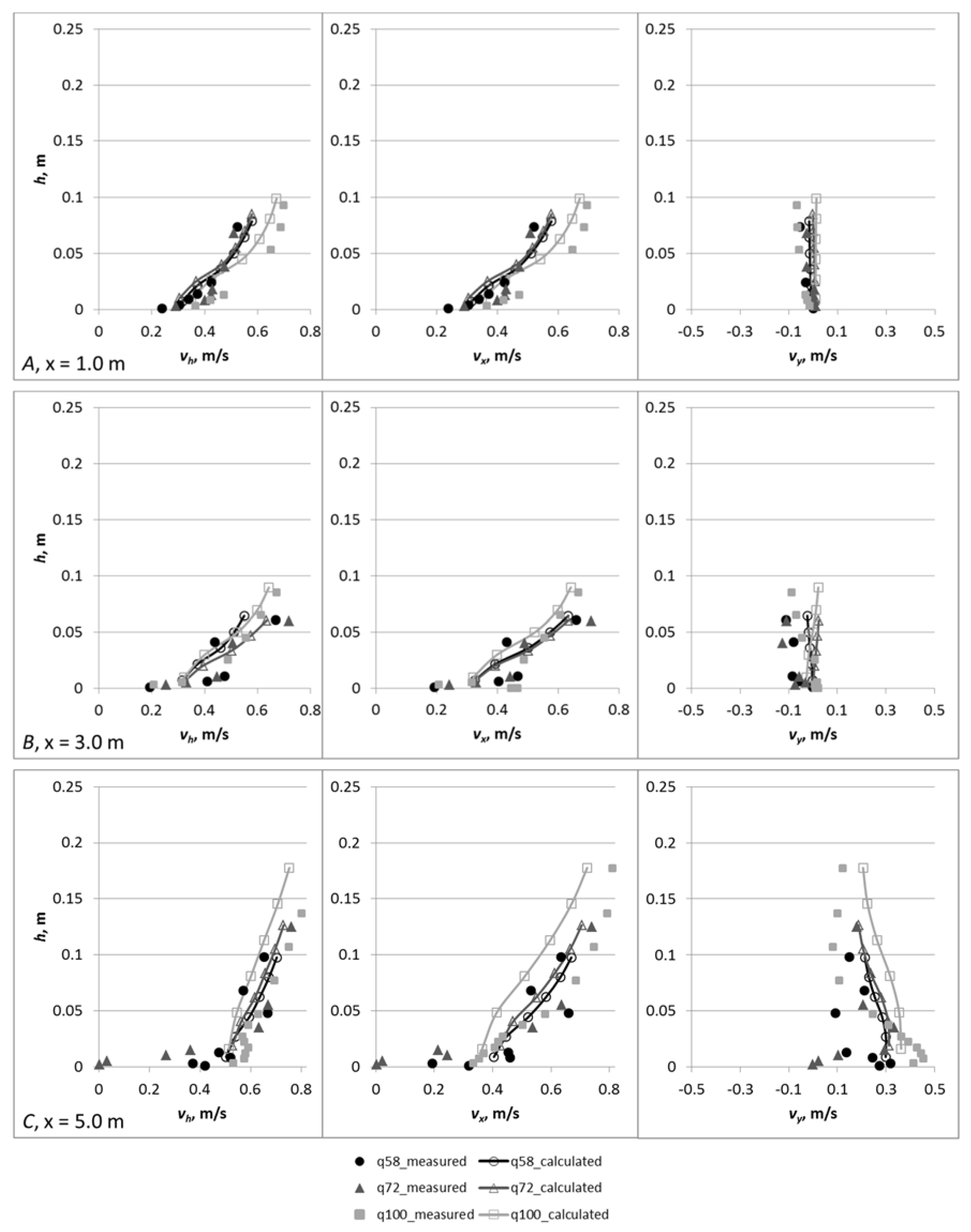

Figure 9.
Measured and simulated equilibrium bed levels at Q = 58 L/s (top: measured, i: vR; ii: Wilcock and Crowe formula; iii: combined approach).
Figure 9.
Measured and simulated equilibrium bed levels at Q = 58 L/s (top: measured, i: vR; ii: Wilcock and Crowe formula; iii: combined approach).
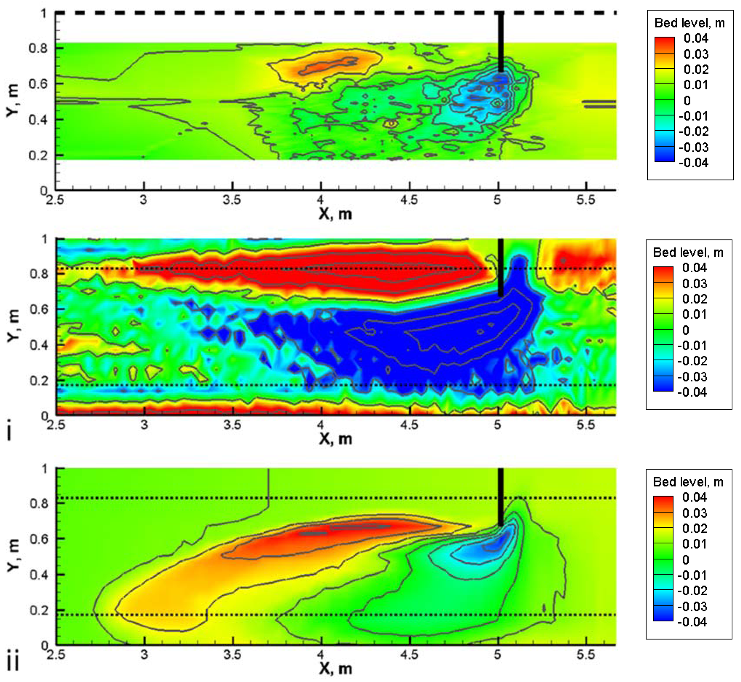

Figure 10.
Measured (circles) and calculated (i: vR; ii: Wilcock and Crowe formula; iii: combined approach) d50 distribution at Q = 58 L/s.
Figure 10.
Measured (circles) and calculated (i: vR; ii: Wilcock and Crowe formula; iii: combined approach) d50 distribution at Q = 58 L/s.
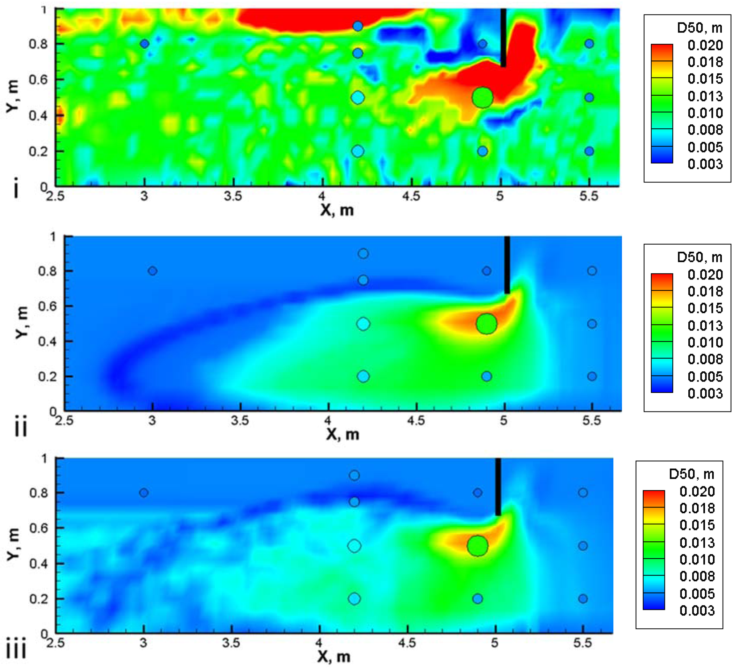
Figure 11.
Measured and simulated equilibrium bed levels at Q = 72 L/s. (top: measured; ii: Wilcock and Crowe formula; iii: combined approach).
Figure 11.
Measured and simulated equilibrium bed levels at Q = 72 L/s. (top: measured; ii: Wilcock and Crowe formula; iii: combined approach).
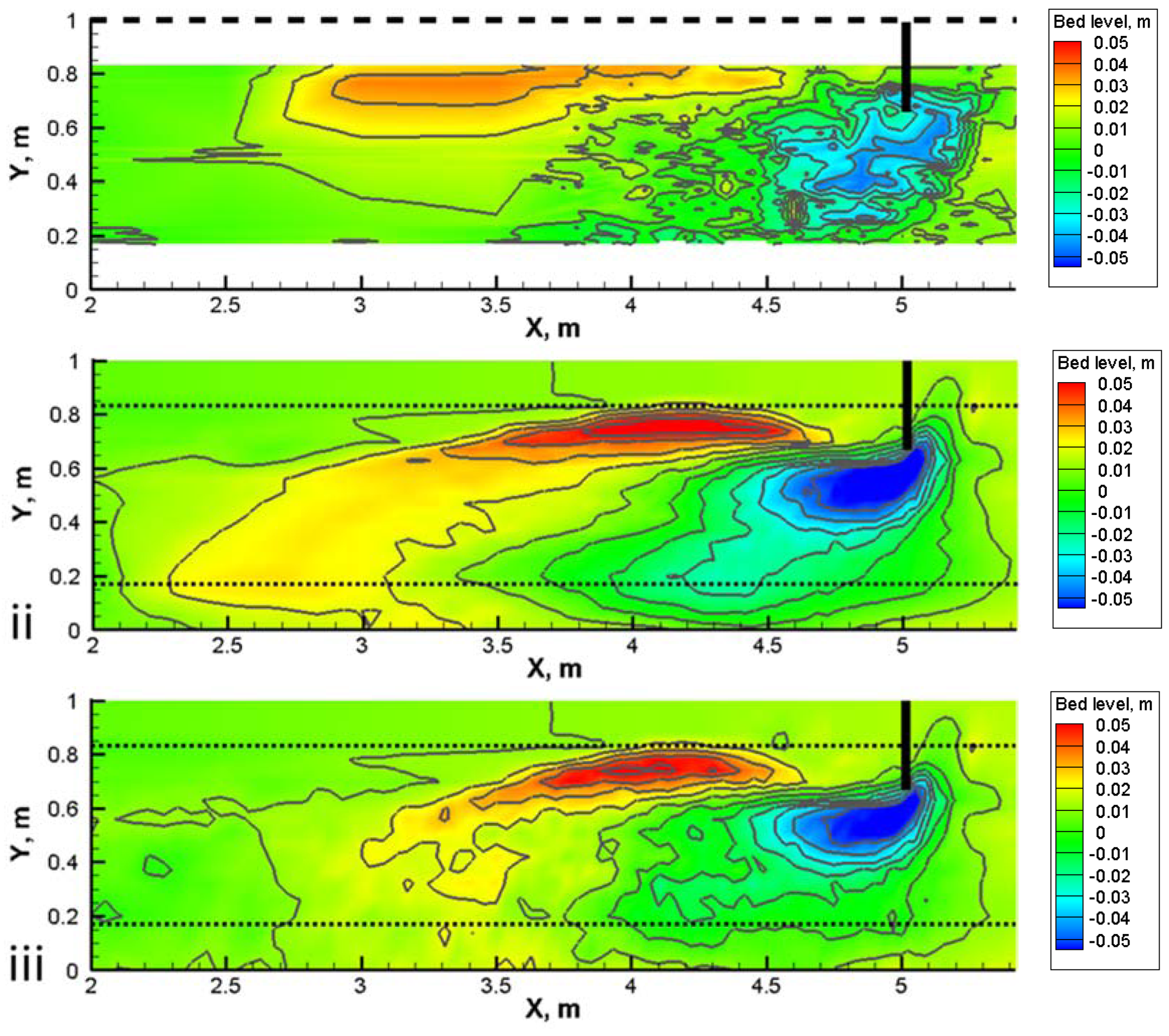
Figure 12.
Measured (circles) and calculated (ii: Wilcock and Crowe formula; iii: combined approach) d50 distribution at Q = 72 L/s.
Figure 12.
Measured (circles) and calculated (ii: Wilcock and Crowe formula; iii: combined approach) d50 distribution at Q = 72 L/s.
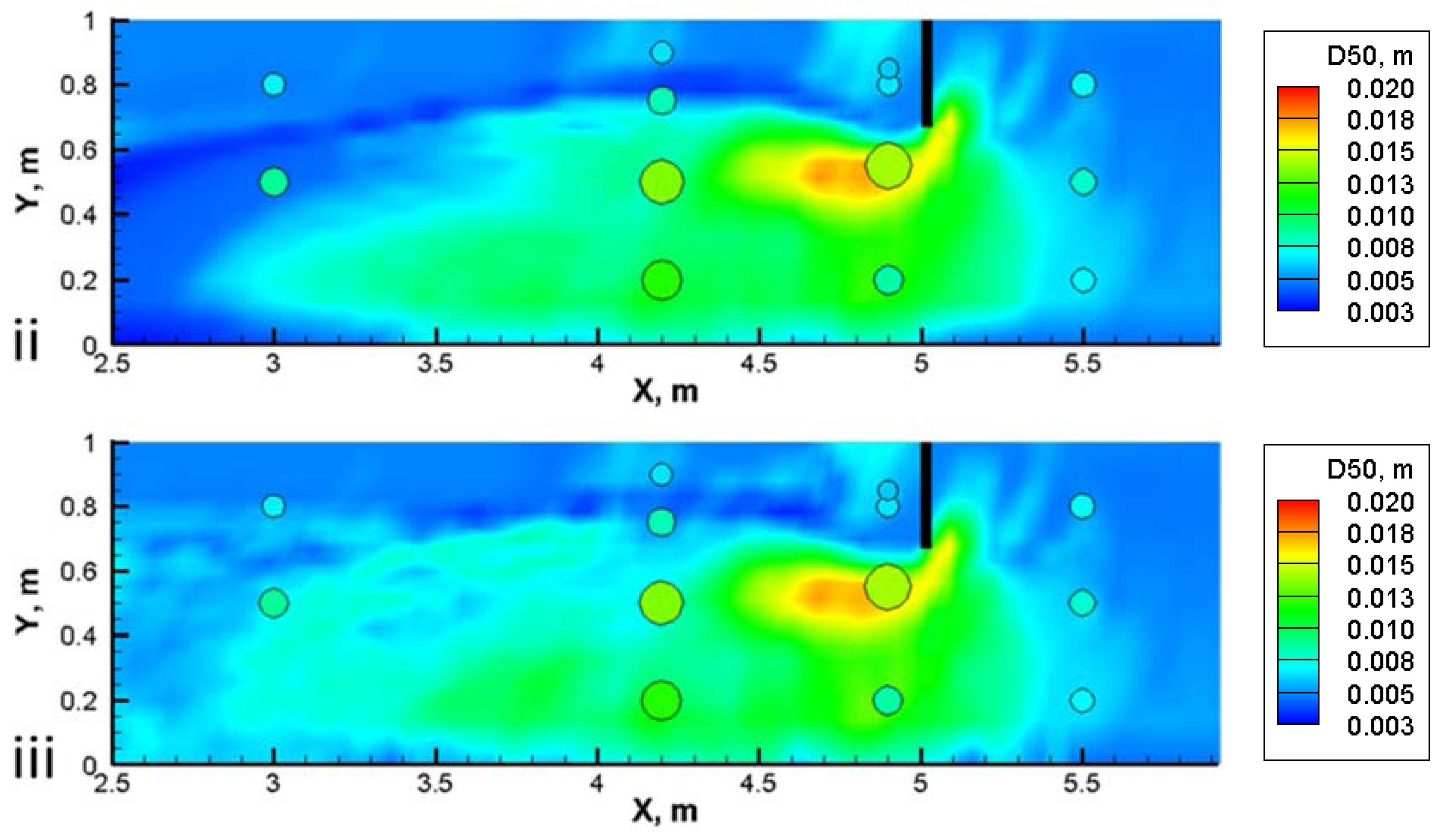
Figure 13.
Measured and simulated equilibrium bed levels at Q = 100 L/s. (top: measured; ii: Wilcock and Crowe formula; iii: combined approach).
Figure 13.
Measured and simulated equilibrium bed levels at Q = 100 L/s. (top: measured; ii: Wilcock and Crowe formula; iii: combined approach).
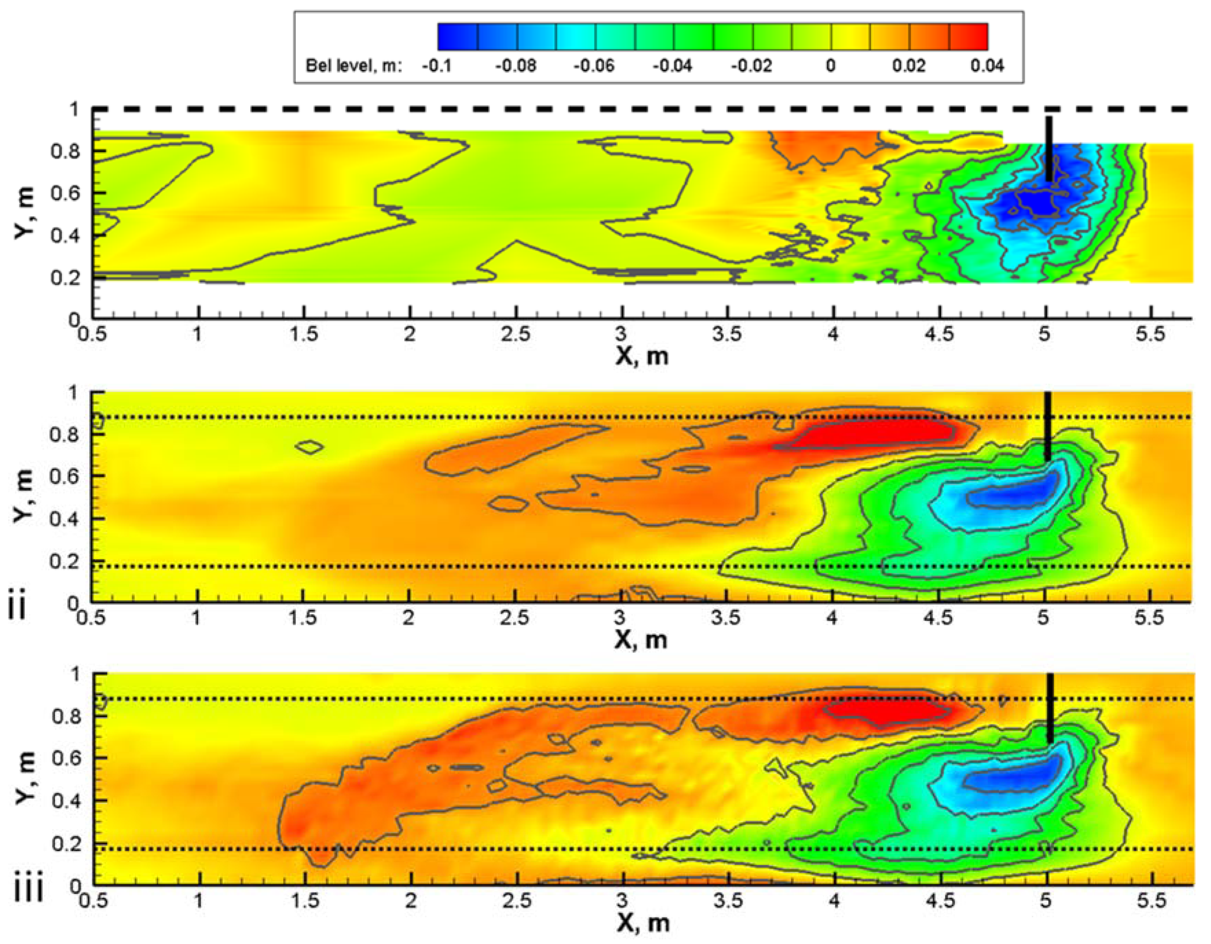
Figure 14.
Measured (circles) and calculated (ii: Wilcock and Crowe formula; iii: combined approach) d50 distribution at Q = 100 L/s.
Figure 14.
Measured (circles) and calculated (ii: Wilcock and Crowe formula; iii: combined approach) d50 distribution at Q = 100 L/s.

Figure 15.
Equilibrium bed levels and d90 = 0.021 m isolines (dotted lines) at Q = 58 L/s, resulting from the combined approach.
Figure 15.
Equilibrium bed levels and d90 = 0.021 m isolines (dotted lines) at Q = 58 L/s, resulting from the combined approach.

Figure 16.
Equilibrium bed shear stress distribution and d90 = 0.021 m isolines (dotted lines) at Q = 58 L/s, resulting from the combined approach.
Figure 16.
Equilibrium bed shear stress distribution and d90 = 0.021 m isolines (dotted lines) at Q = 58 L/s, resulting from the combined approach.

| Q, L/s | hout, m | vavg, m/s | Fr, - | Re, - | τavg, N/m2 | Sbed, - |
|---|---|---|---|---|---|---|
| 58 | 0.137 | 0.42 | 0.15 | 45,500 | 1.9 | 0.0027 |
| 72 | 0.143 | 0.50 | 0.21 | 56,000 | 3.4 | 0.0027 |
| 100 | 0.175 | 0.57 | 0.25 | 74,100 | 3.7 | 0.0027 |
Notes: Q: flow discharge, havg: water depth at the outlet, vavg: averaged flow velocity, Fr: Froude number, Re: Reynolds number, τavg: averaged bed shear stress, Sbed: bed slope.
Table 2.
The Vm/Vc values, where Vm is the calculated and Vc is the measured volume of the deposition form. W&C: Wilcock and Crowe.
| Flow discharge, L/s | Sediment Transport Model | ||
|---|---|---|---|
| Van Rijn | W&C | Combined | |
| 58 | 40.62 | 6.47 | 6.38 |
| 72 | - | 2.12 | 1.10 |
| 100 | - | 0.48 | 0.54 |
Table 3.
The VSh/Vtot values, where VSh is the volume of the shifted and Vtot is the total volume of the total deposition amount.
| Measured | Sediment Transport Model | |
|---|---|---|
| W&C | Combined | |
| 0.39 | 0.09 | 0.54 |
© 2017 by the authors; licensee MDPI, Basel, Switzerland. This article is an open access article distributed under the terms and conditions of the Creative Commons Attribution (CC-BY) license (http://creativecommons.org/licenses/by/4.0/).
Share and Cite
MDPI and ACS Style
Török, G.T.; Baranya, S.; Rüther, N. 3D CFD Modeling of Local Scouring, Bed Armoring and Sediment Deposition. Water 2017, 9, 56. https://doi.org/10.3390/w9010056
AMA Style
Török GT, Baranya S, Rüther N. 3D CFD Modeling of Local Scouring, Bed Armoring and Sediment Deposition. Water. 2017; 9(1):56. https://doi.org/10.3390/w9010056
Chicago/Turabian StyleTörök, Gergely T., Sándor Baranya, and Nils Rüther. 2017. "3D CFD Modeling of Local Scouring, Bed Armoring and Sediment Deposition" Water 9, no. 1: 56. https://doi.org/10.3390/w9010056
Note that from the first issue of 2016, this journal uses article numbers instead of page numbers. See further details here.