
Hydrologic Simulation of a Winter Wheat–Summer Maize Cropping System in an Irrigation District of the Lower Yellow River Basin, China


Abstract
:1. Introduction
2. Materials and Methods
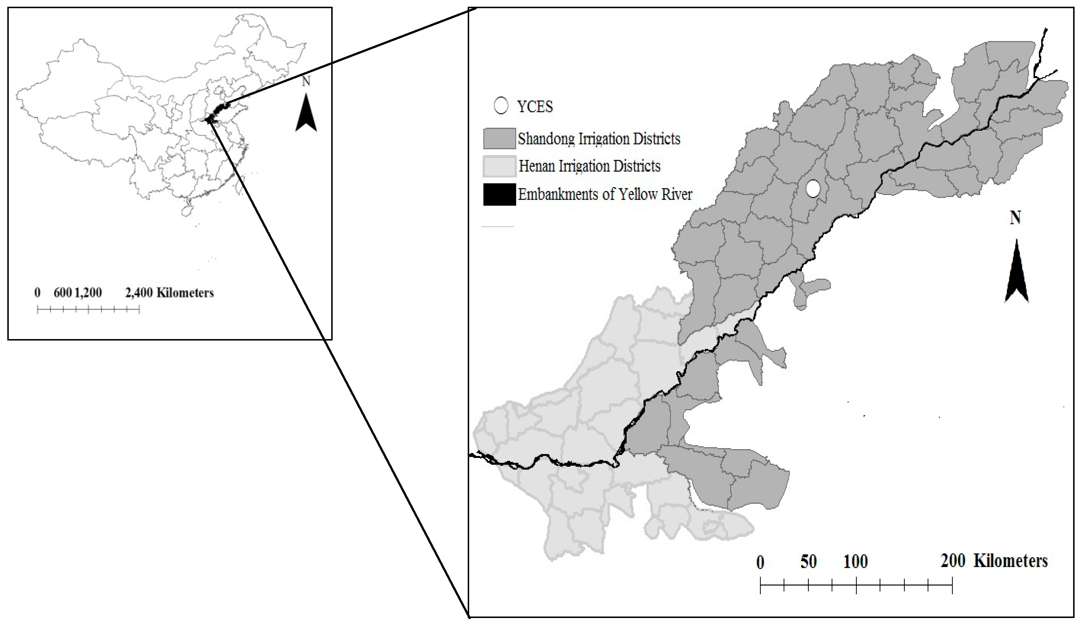
2.1. The Study Area
2.2. Data Preparation
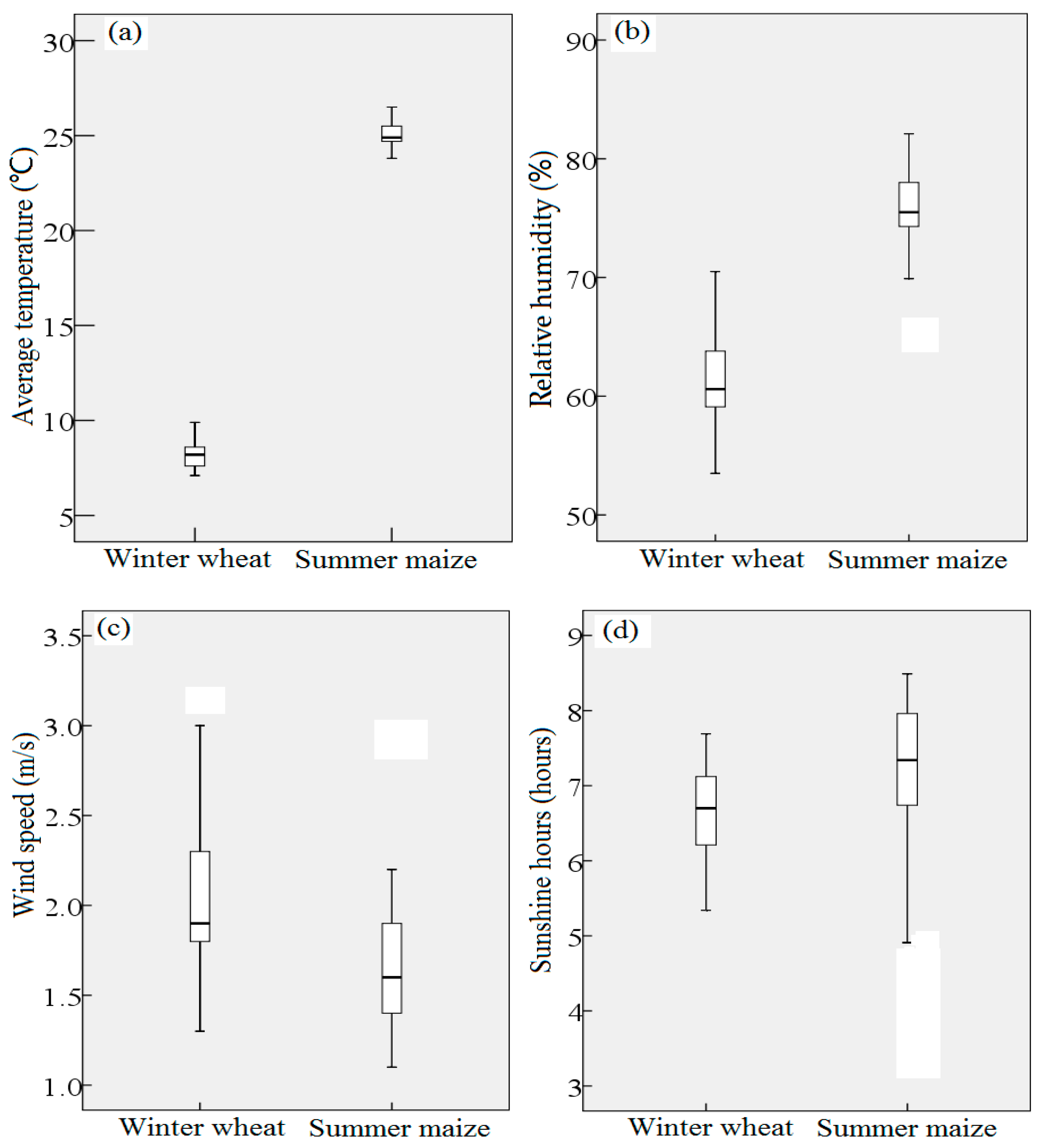
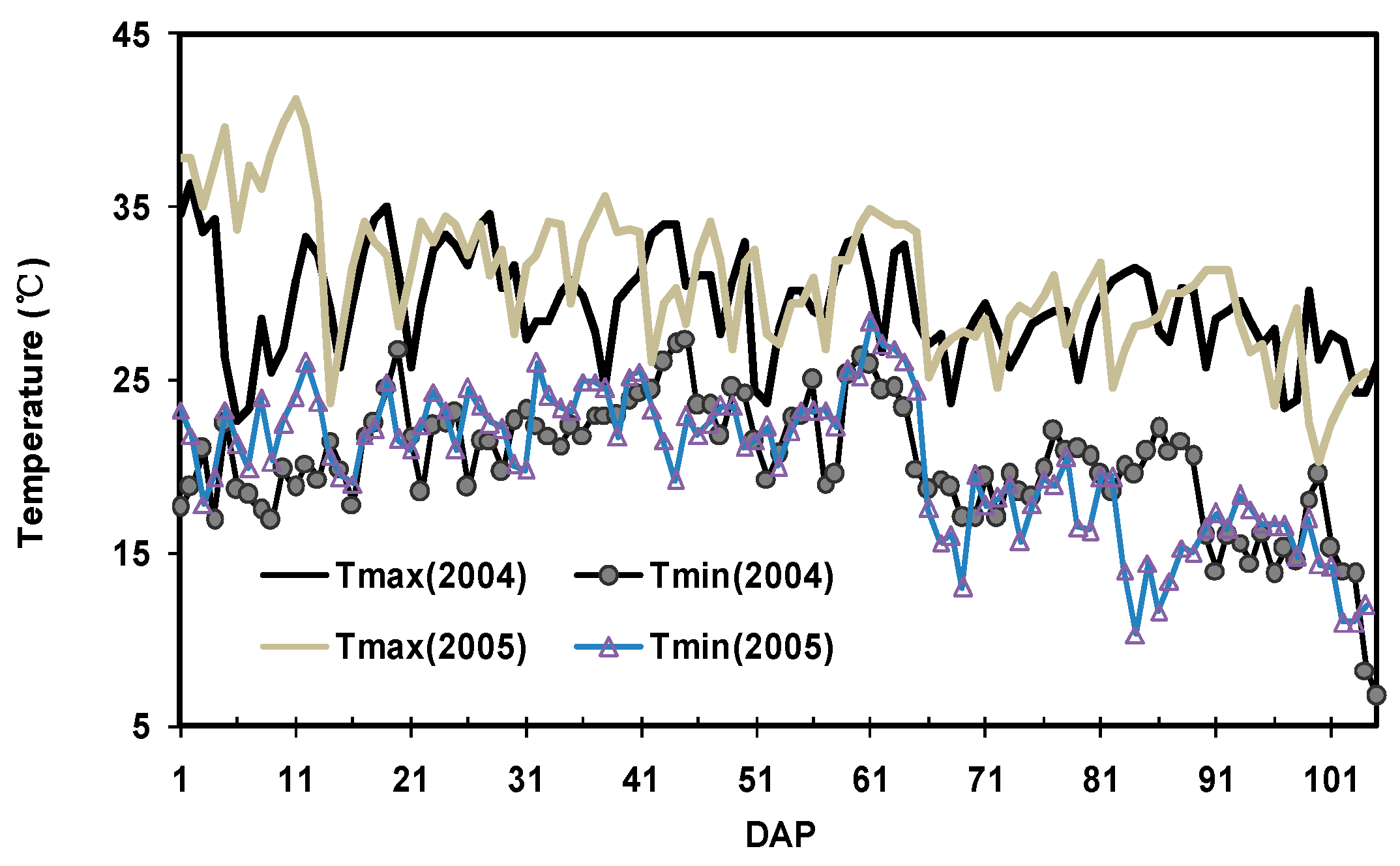
2.2.1. Weather
2.2.2. Crop Parameters
2.2.3. Soil Data
2.2.4. SWAT Model Configuration
2.3. Model Limitations in Simulating Crop Growth
2.4. Scenario Simulations
3. Results
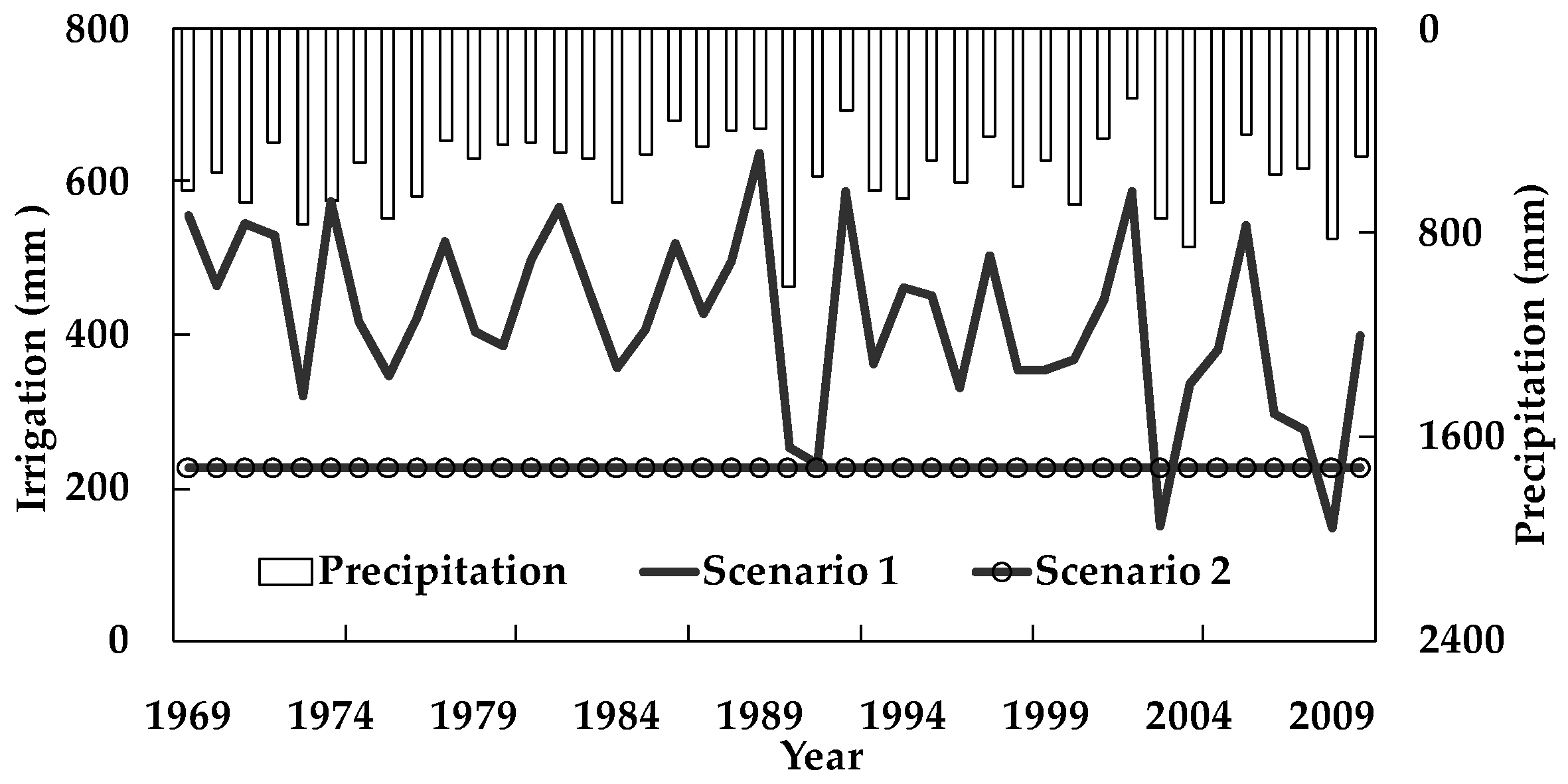
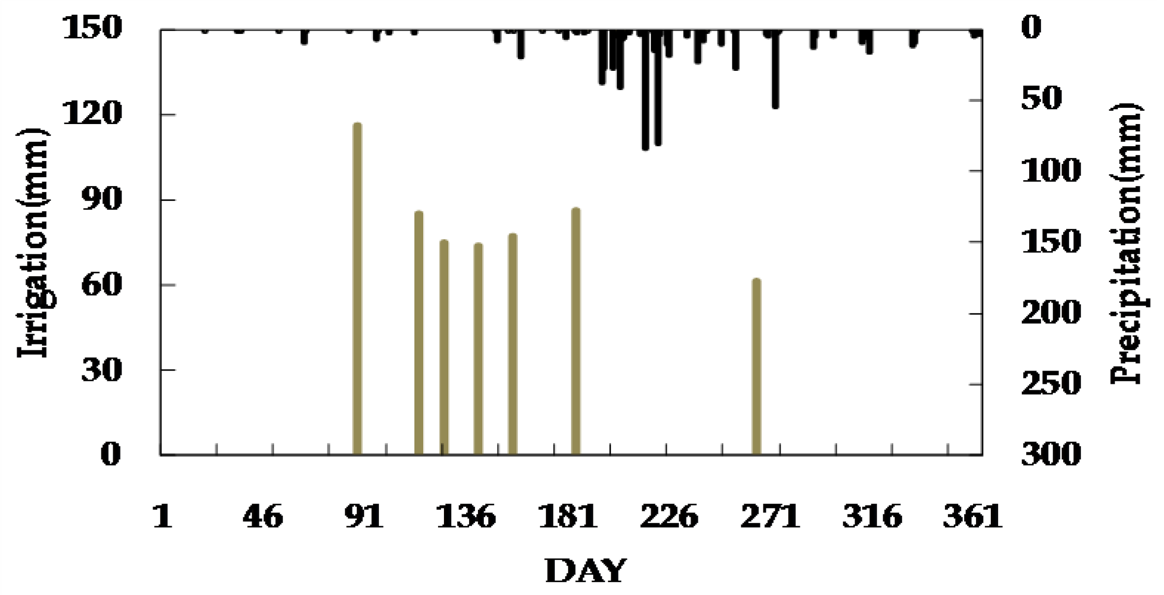
3.1. Irrigation
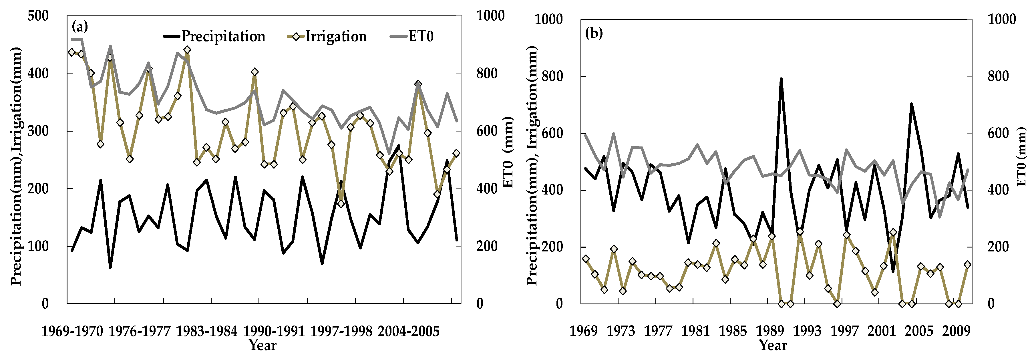
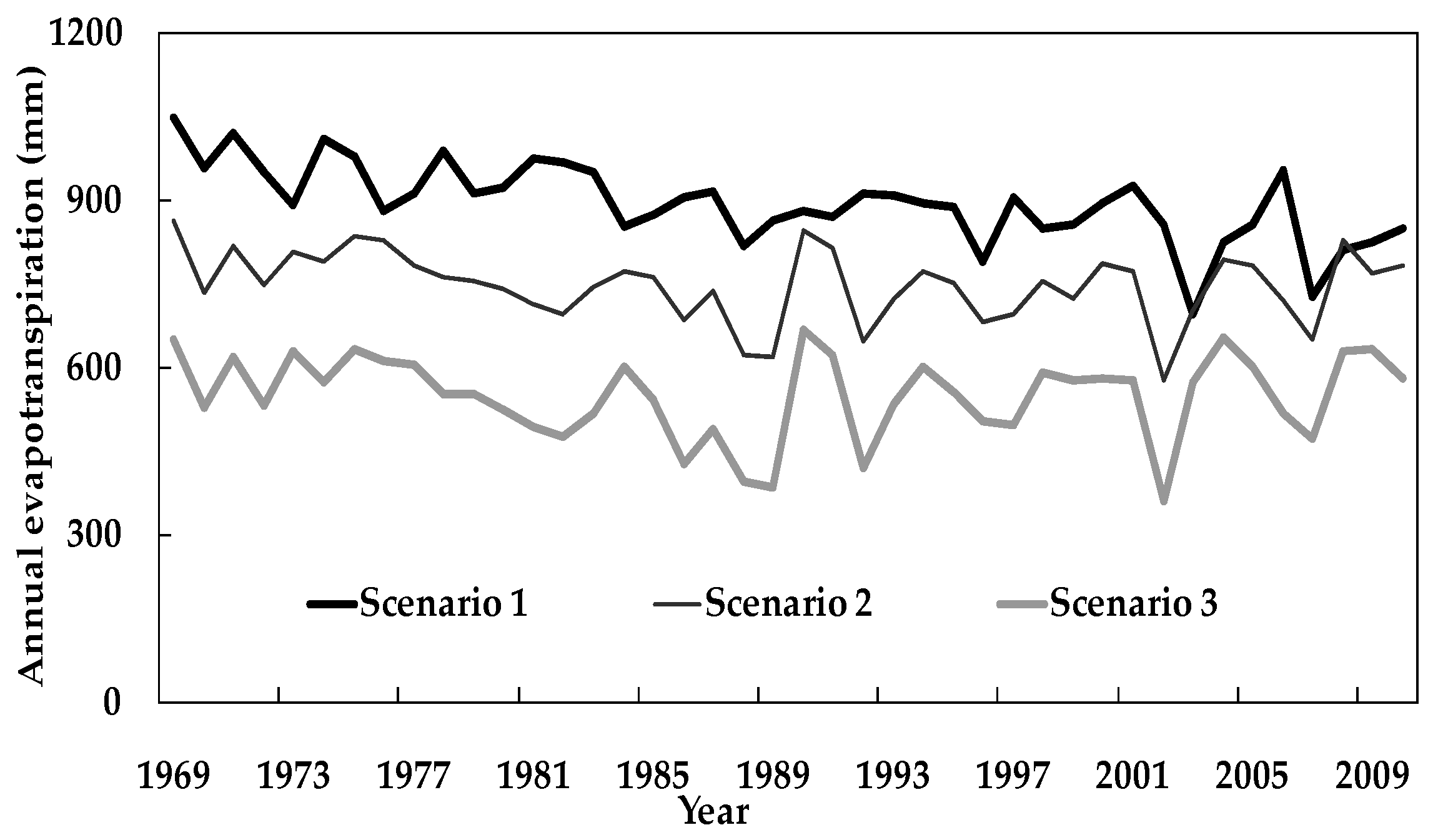
3.2. Evapotranspiration
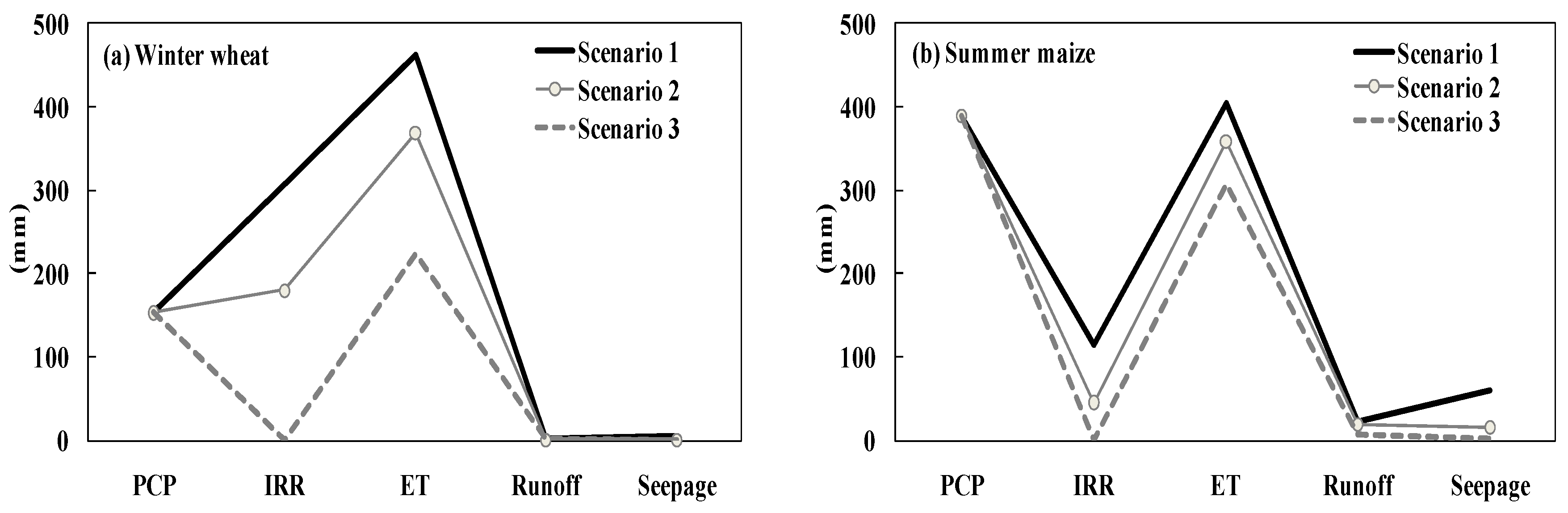
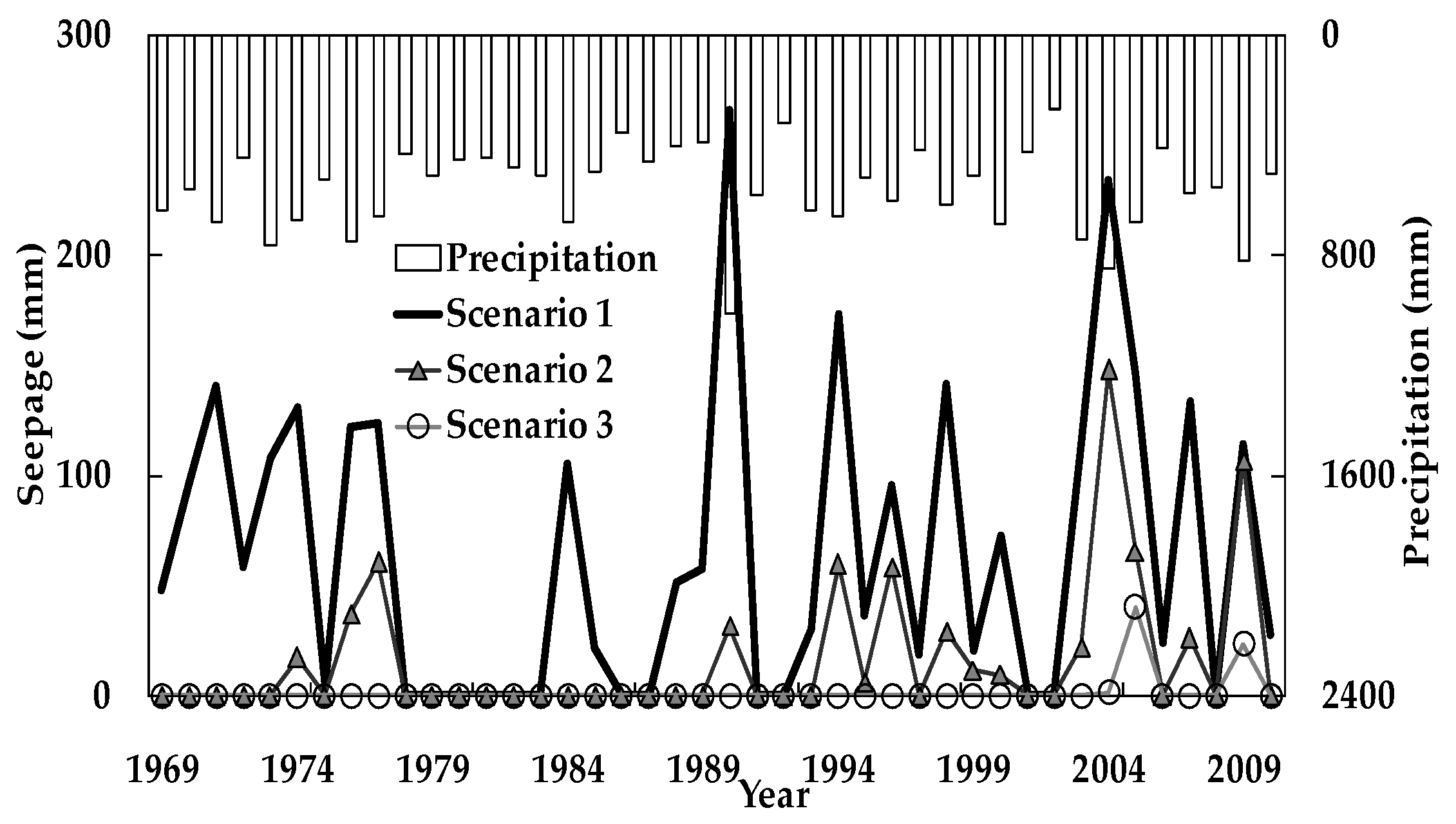
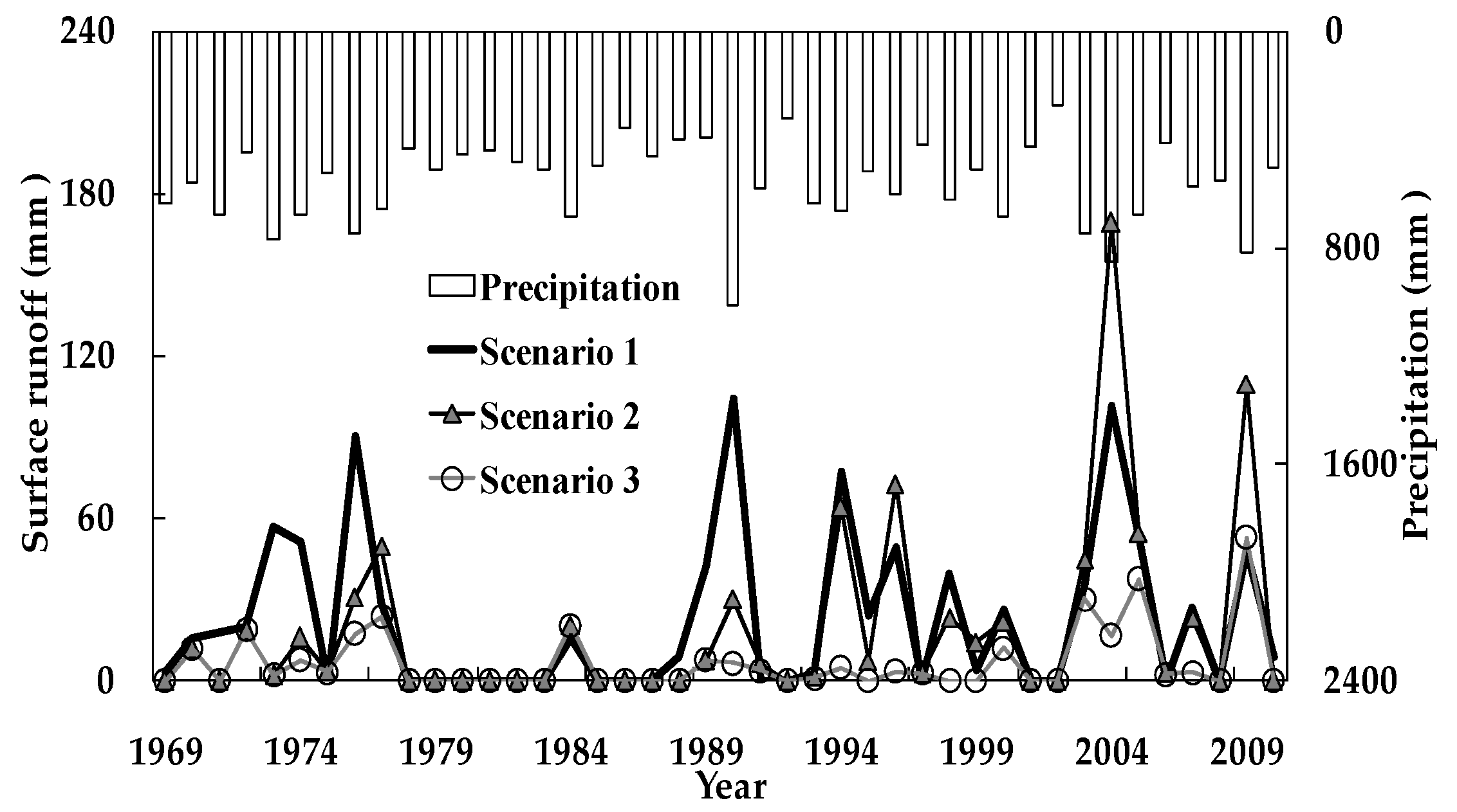
3.3. Seepage and Surface Runoff
3.4. Grain Yield and Water Use Efficiency
3.5. Effects of Meteorological Variables on Irrigation
4. Discussion
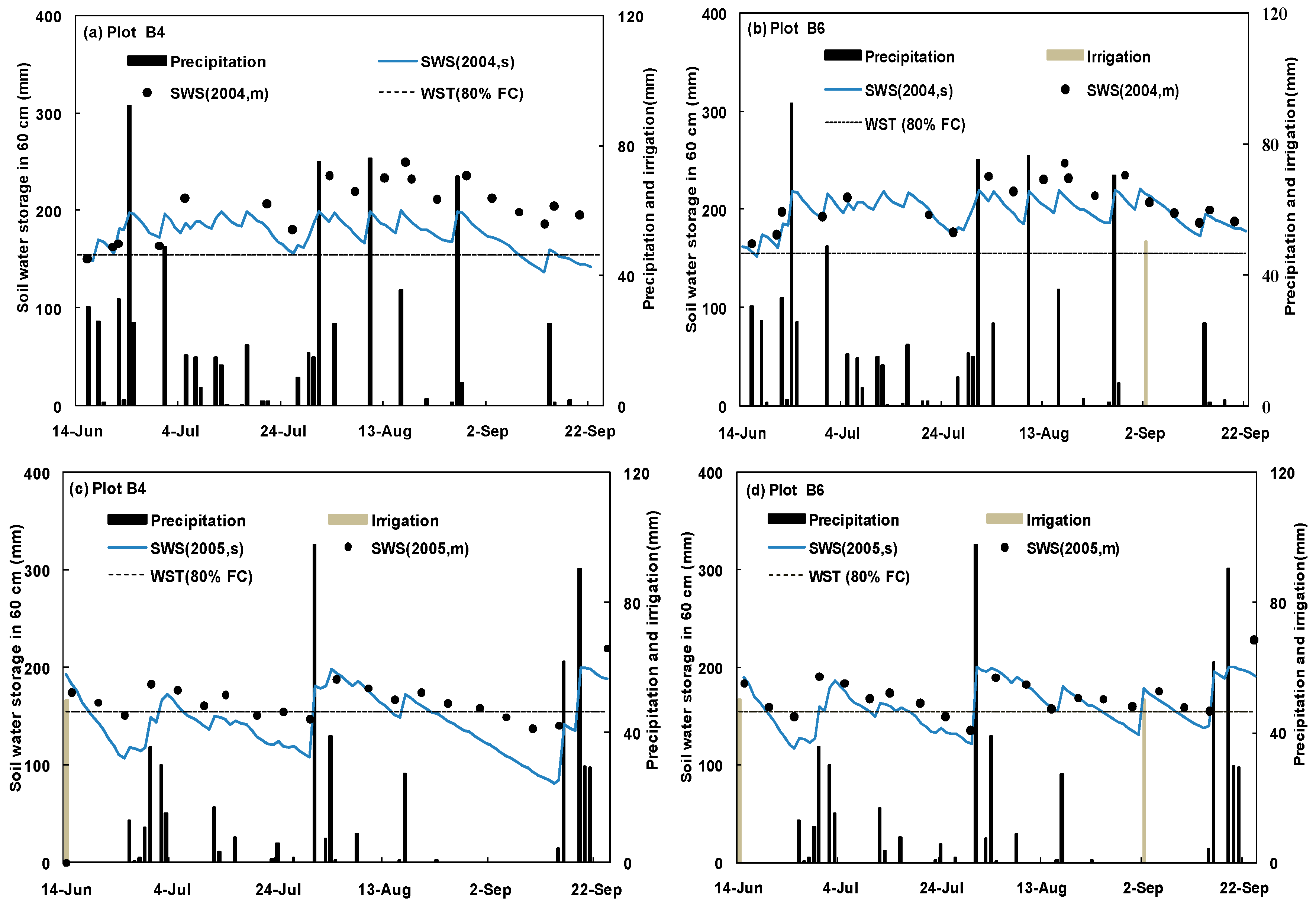
4.1. Validation and Uncertainty Analysis
4.2. Uncertainty of the Results
4.3. Credibility of Results
5. Conclusions
Acknowledgments
Author Contributions
Conflicts of Interest
References
- Young, R.A.; Onstad, C.A.; Borsch, D.D.; Anderson, W.P. AGNPS: A Nonpoint-Source Pollution model for evaluating agricultural watersheds. J. Soil Water Conserv. 1989, 44, 168–173. [Google Scholar]
- Williams, J.R.; Jones, C.A.; Kiniry, J.R.; Spanel, D.A. The EPIC crop growth model. Trans. ASAE 1989, 32, 497–511. [Google Scholar] [CrossRef]
- Arnold, J.G.; Allen, P.M.; Bernhardt, G. A comprehensive surface–ground water flow model. J. Hydrol. 1993, 142, 47–69. [Google Scholar] [CrossRef]
- Neitsch, S.L.; Arnold, J.G.; Kiniry, J.R.; Williams, J.R.; King, K.W. Soil and Water Assessment Tool Theoretical Documentation, Version 2000; Grassland, Soil and Water Research Laboratory, Agricultural Research Service: Temple, TX, USA, 2002.
- Luo, Y.; He, C.; Sophocleous, M.; Yin, Z. Assessment of crop growth and soil water modules in SWAT2000 using extensive field experiment data in an irrigation district of the Yellow River Basin. J. Hydrol. 2008, 352, 139–156. [Google Scholar] [CrossRef]
- Liu, L.; Luo, Y.; He, C.; Lai, J.B.; Li, X.B. Roles of the Combined Irrigation, Drainage, and Storage of the Canal Network in Improving Water Reuse in the Irrigation Districts along the Lower Yellow River, China. J. Hydrol. 2010, 391, 157–174. [Google Scholar] [CrossRef]
- Arnold, J.G.; Allen, P.M. Estimating hydrologic budgets for three Illinois watershed. J. Hydrol. 1996, 176, 57–77. [Google Scholar] [CrossRef]
- Rosenthal, W.D.; Hoffman, D.W. Hydrologic modeling/GIS as an aid in locating monitoring sites. Trans. ASAE 1999, 42, 1591–1598. [Google Scholar] [CrossRef]
- Spruill, C.A.; Workman, S.R.; Taraba, J.L. Simulation of daily and monthly stream discharge from small watersheds using the SWAT model. Trans. ASAE 2000, 43, 1431–1439. [Google Scholar] [CrossRef]
- Chu, T.W.; Shirmohammadi, A.; Montas, H.; Sadeghi, A. Evaluation of the SWAT model’s sediment and nutrient components in the piedomont physiographic region of maryland. Trans. ASAE 2004, 47, 1523–1538. [Google Scholar] [CrossRef]
- Gosain, A.K.; Rao, S.; Srinivasan, R.; Reddy, N.G. Return-flow Assessment for Irrigation Command in the Palleru River Basin using SWAT Model. Hydrol. Process. 2005, 19, 673–682. [Google Scholar] [CrossRef]
- Zhang, A.; Zhang, C.; Fu, G.; Wang, B.; Bao, Z.; Zheng, H. Assessments of impacts of climate change and human activities on runoff with SWAT for the Huifa river basin, northeast China. Water Resour. Manag. 2012, 26, 2199–2217. [Google Scholar] [CrossRef]
- Benaman, J.; Shoemaker, C.; Haith, D. Calibration and validation of soil and water assessment tool on an agricultural watershed in upstate New York. J. Hydrol. Eng. 2005, 10, 363–374. [Google Scholar] [CrossRef]
- Bouraoui, F.; Benabdallah, S.; Jrad, A.; Bidoglio, G. Application of the SWAT model on the Medjerda river basin (Tunisia). Phys. Chem. Earth 2005, 30, 497–507. [Google Scholar] [CrossRef]
- Mishra, A.; Kar, S. Modeling hydrologic processes and NPS pollution in a small watershed in subhumid subtropics using SWAT. J. Hydrol. Eng. 2012, 17, 445–454. [Google Scholar] [CrossRef]
- Bhumika, U.; Madan, K.J.; Arbind, K.V. Assessing climate change impact on water balance components of a river basin using SWAT model. Water Resour. Manag. 2015, 29, 4767–4785. [Google Scholar]
- Van Griensven, A.; Bauwens, W. Application and evaluation of ESWAT on the Dender Basin and the Wister Lake Basin. Hydrol. Process. 2005, 19, 827–838. [Google Scholar] [CrossRef]
- Eckhardt, K.; Arnold, J.G. Automatic calibration of a distributed catchment model. J. Hydrol. 2001, 251, 103–109. [Google Scholar] [CrossRef]
- Ray, S.S.; Dadhwal, V.K. Estimation of crop evapotranspiration of irrigation command area using remote sensing and GIS. Agric. Water Manag. 2001, 49, 239–249. [Google Scholar] [CrossRef]
- Launay, M.; Guerif, M. Assimilating remote sensing data into a crop model to improve predictive performance for spatial applications. Agri. Ecosyst. Environ. 2005, 111, 321–339. [Google Scholar] [CrossRef]
- Groeneveld, D.P.; Baugh, W.M.; Sanderson, J.S.; Cooper, D.J. Annual groundwater evapotranspiration mapped from single satellite scenes. J. Hydrol. 2007, 344, 146–156. [Google Scholar] [CrossRef]
- Santhi, C.; Muttiah, R.S.; Arnold, J.G.; Srinivasan, R. A gis-based regional planning tool for irrigation demand assessment and saving using SWAT. Trans. ASAE 2005, 48, 137–147. [Google Scholar] [CrossRef]
- Cabelguenne, M.; Debaeke, P. Experimental determination and modelling of the soil water extraction capacities of crops of maize, sunflower, soya bean, sorghum and wheat. Plant Soil 1998, 202, 175–192. [Google Scholar] [CrossRef]
- Borrás, L.; Maddonni, G.A.; Otegui, M.E. Leaf senescence in maize hybrids: Plant population, row spacing and kernel set effects. Field Crops Res. 2003, 82, 13–26. [Google Scholar] [CrossRef]
- Leeper, R.A.; Runge, E.C.A.; Walker, W.M. Effect of plant-available stored soil moisture on corn yields: I. Constant climatic conditions. Agron. J. 1974, 66, 723–727. [Google Scholar] [CrossRef]
- Calviño, P.A.; Andrage, F.H.; Sadras, V.O. Maize yield as affected by water availability, soil depth, and crop management. Agron. J. 2003, 95, 275–281. [Google Scholar] [CrossRef]
- Sárvári, M. Impact of nutrient supply, sowing time and plant density on maize yields. Acta Agron. Hung. 2005, 53, 59–70. [Google Scholar] [CrossRef]
- Cross, H.Z.; Zuber, M.S. Prediction of flowering dates in maize based on different methods of estimating thermal units. Agron. J. 1972, 64, 351–355. [Google Scholar] [CrossRef]
- Shaykewich, C.F. An appraisal of cereal crop phenology modeling. Can. J. Plant Sci. 1995, 75, 329–341. [Google Scholar] [CrossRef]
- Yan, W.; Hunt, L.A. An Equation for modelling the temperature response of plants using only the cardinal temperatures. Ann. Bot. 1999, 84, 607–614. [Google Scholar] [CrossRef]
- Lin, Q.; Shi, Y.; Wei, D.B. Relations between soil water and yield formation and determination of Water-saving irrigation scheme in Winter Wheat. Acta Agric. Boreali-Sin. 1998, 13, 1–4. (In Chinese) [Google Scholar]
- Zhu, Z.X.; Zhang, J.C. Crop Water Stress and Drought; Henan Science and Technology Press: Zhengzhou, China, 1991. [Google Scholar]
- Zhang, Y.Q.; Mao, X.S.; Sun, H.Y.; Li, W.J.; Yu, H.N. Effects of drought stress on chlorophyll fluorescence of winter wheat. Chin. J. Eco-Agric. 2002, 10, 13–15. [Google Scholar]
- Zhang, S.; Zhou, X.; Mu, Z.; Shan, L.; Liu, X. Effects of different irrigation patterns on root growth and water use efficiency of maize. Trans. Chin. Soc. Agric. Eng. 2009, 25, 1–6. [Google Scholar]
- Li, J.M.; Inanaga, S.; Li, Z.; Eneji, A.E. Optimizing irrigation scheduling for winter wheat in the North China Plain. Agric. Water Manag. 2005, 76, 8–23. [Google Scholar] [CrossRef]
- Liu, Y.; Cai, J.B.; Cai, L.G.; Pereira, L.S. Analysis of irrigation scheduling and water balance for an irrigation district at lower reaches of the Yellow River. J. Hydraul. Eng. 2005, 36, 701–708. (In Chinese) [Google Scholar]
- Fang, Q.; Ma, L.; Yu, Q.; Ahuja, L.R.; Malone, R.W.; Hoogenboom, G. Irrigation strategies to improve the water use efficiency of wheat–maize double cropping systems in North China Plain. Agric. Water Manag. 2010, 97, 1165–1174. [Google Scholar] [CrossRef]
- Wu, K. Water regime change characteristics and sustainable development of irrigation areas diverted water from Lower Reach of the Huanghe River. J. Irrig. Drain. 2003, 22, 45–47, 66. (In Chinese) [Google Scholar]
- Mann, H.B. Non-parametric tests against trend. Econometrica 1945, 13, 245–259. [Google Scholar] [CrossRef]
- Kendall, M.G. Rank Correlation Methods; Charles Griffin: London, UK, 1975. [Google Scholar]
- Sen, P.K. Estimates of the regression coefficient based on Kendall’s tau. J. Am. Stat. Assoc. 1968, 63, 1379–1389. [Google Scholar] [CrossRef]
- Singh, R.; Van Dam, J.C.; Feddes, R.A. Water productivity analysis of irrigated crops in Sirsa district, India. Agric. Water Manag. 2006, 82, 253–278. [Google Scholar] [CrossRef]
- Zhang, Q.; Xu, C.Y.; Chen, X.H. Reference evapotranspiration changes in China: Natural processes or human influences? Theor. Appl. Climatol. 2011, 103, 479–488. [Google Scholar] [CrossRef]
- Ma, X.N.; Zhang, M.; Li, Y.; Wang, S.; Ma, Q.; Liu, W. Decreasing potential evapotranspiration in the Huanghe watershed in climate warming during 1960–2010. J. Geogr. Sci. 2012, 22, 977–988. [Google Scholar] [CrossRef]
- Chen, B.; Ouyang, Z.; Cheng, W.X.; Liu, L.P. Water consumption for winter wheat and summer maize in the North China Plain in Recent 50 Years. J. Nat. Resour. 2012, 27, 1186–1199. (In Chinese) [Google Scholar]
- Neitsch, S.L.; Arnold, J.G.; Kiniry, J.R.; Williams, J.R. Soil and Water Assessment Tool Theoretical Documentation, Version 2009; Grassland, Soil and Water Research Laboratory, Agricultural Research Service: Temple, TX, USA, 2011.
- Hu, W.; Yan, C.R.; Li, Y.C.; Liu, Q. Impacts of climate change on winter wheat growing period and irrigation water requirements in the north china plain. Acta Ecol. Sin. 2014, 34, 2367–2377. (In Chinese) [Google Scholar] [CrossRef]
- Huan, H.J.; Yang, Z.Q.; Liu, Y.; Xia, F.H.; Yang, K. Temporal and spatial variation of water deficit and irrigation requirement for corn in the middle of Shandong province in China. Jiangsu Agric. Sci. 2016, 44, 342–347. (In Chinese) [Google Scholar]
- Song, Z.W.; Zhang, H.L.; Snyder, R.L.; Anderson, F.E.; Chen, F. Distribution and trends in reference evapotranspiration in the North China Plain. J. Irrig. Drain. Eng. 2010, 136, 240–247. [Google Scholar] [CrossRef]
- Liu, X.Y.; Li, Y.Z.; Hao, W.P. Trend and causes of water requirement of main crops in North China in recent 50 years. Trans. CSAE 2005, 21, 155–159. (In Chinese) [Google Scholar]
- Yang, X.L.; Song, Z.W.; Wang, H.; Shi, Q.H.; Chen, F.; Chu, Q.Q. Spatio-temporal variations of winter wheat water requirement and climatic causes in Huang-Huai-Hai Farming Region. Chin. J. Eco-Agric. 2012, 20, 356–362. (In Chinese) [Google Scholar] [CrossRef]
- Yang, X.L.; Huang, J.; Chen, F.; Chu, Q.Q. Comparison of temporal and spatial variation of water requirement of corn in Huang-Huai-Hai farming system region. J. China Agric. Univ. 2011, 16, 26–31. (In Chinese) [Google Scholar]


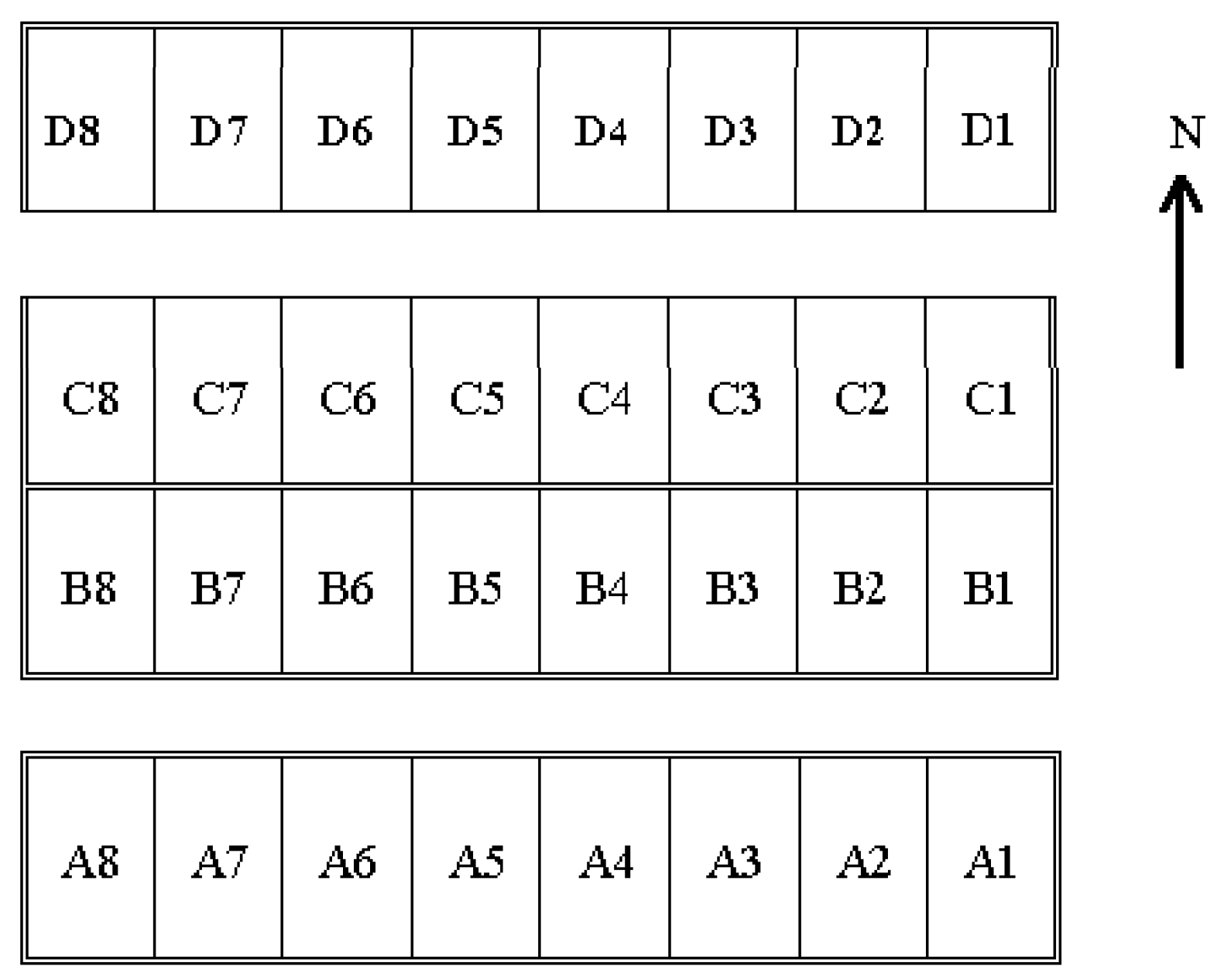
| 1 | 2 | 3 | 4 | 5 | 6 | 7 | 8 | Plant Density | |
|---|---|---|---|---|---|---|---|---|---|
| A | Treatment I: No irrigation | Treatment II: 40% FC | ND | ||||||
| B | Treatment III: 60% FC | Treatment IV: 80% FC | |||||||
| C | Treatment V: No irrigation | Treatment VI: 40% FC | 75% ND | ||||||
| D | Treatment VII: 60% FC | Treatment VIII: 80% FC | |||||||
| 1 | 2 | 3 | 4 | 5 | 6 | 7 | 8 | Plant Density | |
|---|---|---|---|---|---|---|---|---|---|
| A | Treatment I: No irrigation | Treatment II: 60% FC | 150% ND | ||||||
| B | Treatment III: No irrigation | Treatment IV: 60% FC | 133% ND | ||||||
| C | Treatment V: No irrigation | Treatment VI: 60% FC | 117% ND | ||||||
| D | Treatment VII: No irrigation | Treatment VIII: 60% FC | ND | ||||||
| Growth Season | PHU (°C) a | LAImax b | frphu,1 c | frlai,1 d | frphu,2 e | frlai,2 f | frphu,sen g |
|---|---|---|---|---|---|---|---|
| Winter wheat | 1852.6 | 8.5 | 0.20 | 0.20 | 0.45 | 0.96 | 0.48 |
| Summer maize | 1850.9 | 5.0 | 0.35 | 0.30 | 0.50 | 0.95 | 0.60 |
| Depth (mm) | 50.0 | 300.0 | 600.0 | 700.0 | 800.0 | 1200.0 | 1800.0 |
|---|---|---|---|---|---|---|---|
| Bulk density (g/cm3) | 1.45 | 1.50 | 1.46 | 1.50 | 1.45 | 1.45 | 1.45 |
| Soil AWC a (mm/mm) | 0.26 | 0.26 | 0.24 | 0.24 | 0.22 | 0.22 | 0.22 |
| Ksat b (mm/h) | 150.0 | 150.0 | 150.0 | 150.0 | 150.0 | 150.0 | 150.0 |
| Content of organic carbon (%) | 2.5 | 1.0 | 0.0 | 0.0 | 0.0 | 0.0 | 0.0 |
| Content of clay (%) | 11.8 | 18.8 | 18.5 | 18.5 | 19.5 | 14.0 | 15.7 |
| Content of silt (%) | 66.7 | 67.8 | 70.6 | 70.6 | 70.6 | 70.6 | 70.6 |
| Content of sand (%) | 21.5 | 13.4 | 10.9 | 10.9 | 9.9 | 15.4 | 13.7 |
| Growth Season | A1–A4 | A5–A8 | B1–B4 | B5–B8 | C1–C4 | C5–C8 | D1–D4 | D5–D8 |
|---|---|---|---|---|---|---|---|---|
| 2004 | −22.7 | −19.9 | −18.7 | −20.4 | −25.4 | −19 | −10.3 | −1.6 |
| 2005 | −1.1 | −8.1 | −18.7 | −22.6 | −18.3 | −15.5 | −1.7 | 10.4 |
| Growth Season | PHU (°C) a | LAImax b | frphu,1 c | frlai,1 d | frphu,2 e | frlai,2 f | frphu,sen g |
|---|---|---|---|---|---|---|---|
| 2004 | 1750.4 | 5 | 0.25 | 0.27 | 0.40 | 0.95 | 0.55 |
| 2005 | 1870.4 | 5 | 0.37 | 0.30 | 0.55 | 0.95 | 0.65 |
| Variable | Winter Wheat | Summer Maize | Annual | |||
|---|---|---|---|---|---|---|
| Z | β | Z | β | Z | β | |
| Average temperature | 3.88 * | 0.04 | 2.10 ** | 0.02 | - | - |
| Wind speed | −3.01 * | −0.02 | −1.76 ** | −0.01 | - | - |
| Relative humidity | 2.53 * | 0.14 | 0.61 | 0.02 | - | - |
| Sunshine hours | −3.80 * | −0.03 | −3.79 * | -0.04 | - | - |
| ET0 | −4.71 * | −4.55 | −3.60 * | −2.69 | −5.58 * | −3.95 |
| Precipitation | 0.86 | 0.53 | −0.55 | −0.81 | −0.14 | −0.35 |
| Irrigation | −3.13 * | −2.91 | −0.69 | −0.33 | −2.48 * | −3.80 |
| Crop | Statistic | Scenario 1 | Scenario 2 | Scenario 3 | |||
|---|---|---|---|---|---|---|---|
| Yield | WUE a | Yield | WUE | Yield | WUE | ||
| (kg·ha−1) | (kg·m−3) | (kg·ha−1) | (kg·m−3) | (kg·ha−1) | (kg·m−3) | ||
| Winter wheat | Max | 6272 | 1.46 | 5697 | 1.81 | 4460 | 2.06 |
| Min | 3903 | 0.86 | 3142 | 0.79 | 1007 | 0.49 | |
| Mean | 5284 | 1.15 | 4709 | 1.29 | 2548 | 1.15 | |
| Stdev | 575 | 0.14 | 598 | 0.21 | 895 | 0.36 | |
| CV | 0.11 | 0.12 | 0.13 | 0.17 | 0.35 | 0.31 | |
| Summer maize | Max | 7955 | 1.87 | 7522 | 1.88 | 7417 | 2.12 |
| Min | 3204 | 1.06 | 3206 | 1.06 | 2508 | 1.13 | |
| Mean | 6146 | 1.51 | 5265 | 1.46 | 4963 | 1.61 | |
| Stdev | 1046 | 0.17 | 1029 | 0.18 | 1143 | 0.23 | |
| CV | 0.17 | 0.11 | 0.20 | 0.13 | 0.23 | 0.15 | |
| Variable | Winter Wheat | Summer Maize | ||
|---|---|---|---|---|
| Correlation Coefficient | p Values | Correlation Coefficient | p Values | |
| Average temperature | −0.261 | 0.103 | 0.272 | 0.081 |
| Wind speed | 0.696 | 0.000 * | 0.409 | 0.009 * |
| Relative humidity | −0.585 | 0.000 * | −0.738 | 0.000 * |
| Sunshine hours | 0.553 | 0.000 * | 0.813 | 0.000 * |
| Variable | Winter Wheat | Summer Maize | ||
|---|---|---|---|---|
| Correlation Coefficient | p Values | Correlation Coefficient | p Values | |
| ET0 | 0.806 | 0.000 * | 0.515 | 0.000 * |
| Precipitation | −0.430 | 0.005* | −0.276 | 0.077 |
| Parameters | PET | IWR | Significance |
|---|---|---|---|
| FRGRW1 | 1 | 1 | Fraction of PHU at point 1 on the optimal leaf area development curve |
| BLAI | 2 | 4 | Maximum potential leaf area index |
| DLAI | 3 | 2 | Fraction of growing season when leaf area declines |
| FRGRW2 | 4 | 7 | Fraction of PHU at point 2 on the optimal leaf area development curve |
| LAIMX2 | 5 | 5 | Fraction of the maximum LAI at point 2 on the optimal leaf area development curve |
| LAIMX1 | 6 | 6 | Fraction of the maximum LAI at point 1 on the optimal leaf area development curve |
| Soil AWC | 7 | 3 | Soil available water content |
| Bulk density | 8 | 8 | Soil bulk density |
| Simulated PET of Winter Wheat | Simulated IWR of Winter Wheat | Simulated PET of Summer Maize | Simulated IWR of Summer Maize | |
|---|---|---|---|---|
| Percent within the 95% CI | 98% | 93% | 93% | 100% |
© 2017 by the authors; licensee MDPI, Basel, Switzerland. This article is an open access article distributed under the terms and conditions of the Creative Commons Attribution (CC-BY) license (http://creativecommons.org/licenses/by/4.0/).
Share and Cite
Liu, L.; Ma, J.; Luo, Y.; He, C.; Liu, T. Hydrologic Simulation of a Winter Wheat–Summer Maize Cropping System in an Irrigation District of the Lower Yellow River Basin, China. Water 2017, 9, 7. https://doi.org/10.3390/w9010007
Liu L, Ma J, Luo Y, He C, Liu T. Hydrologic Simulation of a Winter Wheat–Summer Maize Cropping System in an Irrigation District of the Lower Yellow River Basin, China. Water. 2017; 9(1):7. https://doi.org/10.3390/w9010007
Chicago/Turabian StyleLiu, Lei, Jianqin Ma, Yi Luo, Chansheng He, and Tiegang Liu. 2017. "Hydrologic Simulation of a Winter Wheat–Summer Maize Cropping System in an Irrigation District of the Lower Yellow River Basin, China" Water 9, no. 1: 7. https://doi.org/10.3390/w9010007