Assessment on the Effect of Climate Change on Streamflow in the Source Region of the Yangtze River, China

Abstract

Tuotuo River basin, known as the source region of the Yangtze River, is the key area where the impact of climate change has been observed on many of the hydrological processes of this central region of the Tibetan Plateau. In this study, we examined six Global Climate Models (GCMs) under three Representative Concentration Pathways (RCPs) scenarios. First, the already impacted climate change was analyzed, based on the historical data available and then, the simulation results of the GCMs and RCPs were used for future scenario assessments. Results indicated that the annual mean temperature will likely be increased, ranging from −0.66 °C to 6.68 °C during the three future prediction periods (2020s, 2050s and 2080s), while the change in the annual precipitation ranged from −1.18% to 66.14%. Then, a well-known distributed hydrological soil vegetation model (DHSVM) was utilized to evaluate the effects of future climate change on the streamflow dynamics. The seasonal mean streamflows, predicted by the six GCMs and the three RCPs scenarios, were also shown to likely increase, ranging from −0.52% to 22.58%. Watershed managers and regulators can use the findings from this study to better implement their conservation practices in the face of climate change.

1. Introduction

Climate change and variability has been known as an indisputable observation that has recently attracted substantial attentions from governmental institutions around the world [1,2]. Indeed, The Fourth Assessment Report of the Intergovernmental Panel on Climate Change (IPCC AR4) [3,4,5] has pointed out that the global warming will lead to speeding up of the glacial melting process, impacting global hydrologic cycle, and change the distribution patterns of the future precipitations. Compared with the IPCC AR4, the IPCC AR5 [6] had a great innovative warning, it not only pointed out the possible scenarios of atmospheric radiation forces, but also made daring predictions for the near future climate change impacts that the public and government around the world should seriously be concerned. Accordingly, other reports have also warned that the existing and the future water resources availability around the world have been and will be severely impacted by climate change [7,8,9,10]. Thus, assessing the extent of climate change impacts on hydrology of the river basins as well as other water resources, both surface and groundwater, is of a great significance for water resources management and the findings are crucial for decision making on the potential change for the future utilization of these valuable water resources.

To systematically study the effects of climate change on future hydrological processes, Global Climate Models (GCMs) have been proven to be the effective tools for simulating scenarios of both current and the future climate patterns. The model’s outputs could also be used as the critical and useful inputs for application of local hydrological models. However, the spatial mismatch problem between the GCMs and the hydrological models is the key concerns for climate change assessment and the direct use of the GCMs outputs is difficult to be accurately associated with the regional climate change impacts. Thus, a downscaling method is needed to resolve this mismatch issue between the outputs of the GCMs and the inputs for the local hydrologic models [11,12]. There are several kinds of statistical downscaling methods like SDSM, CF, LARS-WG and BSCD, etc. The relative performance of different WGs was evaluated by Semenov [13] who indicated that LARS-WG is better than WGEN at reproducing monthly temperature and precipitation means across the USA, Europe and Asia due to a greater number of parameters and the use of more complex distributions [14]. Luo et al. [15] pointed out that LARS-WG displayed a better performance in simulating the wet-dry series than SDSM and other methods. Etemadi et al. [16] found that the LARSWG method gave a better performance at reproducing various statistical characteristics of observed data at a 95% confidence level than SDSM, which meant that LARS-WG gave less uncertainty. Thus, the LARS-WG is the ideal model for downscaling work in this study. Therefore, the LARS-WG has been successfully applied in many recent studies [17,18], primarily because of its the convenience use and the feasibility of method.

In particular, in the northwest region of the China, climate change impacts have greatly affected the local water resources and the environment. Especially over the Tibetan Plateau, known as “the third pole of the world”, with an average altitude of over 4000 m. During the past 30 years, the Tibetan Plateau has been experiencing significant climate change impacts, which have led to the many related hydrology and climatic variables changes, such as the change in atmospheric conditions, hydrologic water cycle, and the local environmental and water quantity, as well as the basin’s streamflows and lakes water levels [19]. Some of the recently related studies have also shown that the temperature of the high elevation areas have risen more than that of the lower elevation areas, thus even the slight change in the hydrologic cycle, have resulted in significant impact on the weather pattern as well as the management strategies of water resources in the Tibetan Plateau areas [20,21,22,23]. For example, Gao et al. [20] used the HBV-light model to simulate glacier streamflow and glacier mass balance (GMB) in a small watershed in the central Tibetan Plateau. They also used the regional climate model ECHAM5/MPI-OM to simulate the climate change effects on the streamflow and the GMB for the next 40 years. The results showed that the annual runoff would increase while the mean ice elevation may decrease due to the continuous rising temperature. Li et al. [21] used twenty GCMs and two scenarios to study the impact of climate change on the streamflow pattern in the Yellow River region. Their simulation results showed that in both, the Yangtze River and the Yellow River region, the streamflow levels are likely to increase due to the increase in precipitation amounts and the rise in temperature.

The Yangtze River basin is one of the most important region for agricultural and industrial production in China and the Tuotuo River basin, known as the headwater of the Yangtze River, has recently observed obvious hydrological changes under climate changes [24,25]. Therefore, research is needed to better understand the specific impacts of climate change on hydrology and water resources in this plateau, especially for the future wise water resources management decisions in this region.

In this paper, we applied a distributed hydrological soil vegetation model (DHSVM) to detect the effects of climate changes on hydrology in the source region of the Yangtze River for the future period (2011–2100), based on six GCMs and three RCPs. One main objective is to study the long-term changes in hydrology, including evapotranspiration. The second objective is to analyze the uncertainties associated with the climate change impact scenarios and hydrological modelling in the study area.

2. Materials and Methods

2.1. Study Area

The Tuotuo River basin (shown in Figure 1) is considered as the headwater of the Yangtze River, located in the central part of the Tibetan Plateau region in China. The area of this basin is approximately 15,000 km² and is bounded by the coordination of 89°48′ E–92°54′ E and 33°22′ N–35°12′ N. The study area also features some high elevations zones with the average elevation of nearly 4500 m above the sea level. On average, over 50% of the study area is covered by alpine and sub-alpine plain grass, 2.4% of this basin is covered by the glacier. This vast territorial area are with some high elevations, changeable climate, and low temperature all over the year, which make up the rugged environment characteristics of the Tuotuo River basin.

Due to the spatial location of the area, the annual mean temperature, during the past 30 years, was around −4.2 °C, the highest average temperature of 7.5 °C occurred during the July months, and the extreme minimum temperature observed to be nearly −33.8 °C. The basin normally receives annual mean precipitation of 261 mm and over 70% of annual precipitation occurs normally between June and October with June and August being usually the wettest months of the year. There is only one hydrological station (the Tuotuo River station) exists in the study area due to the harsh climatic conditions.

2.2. Databases Sources

2.2.1. Digital Elevation Model Data

The Digital Elevation Model (DEM) data with 90 m resolution were obtained from the CGIAR-CSI (http://srtm.csi.cgiar.org). The data were used to delineate the watershed boundaries and to generate the river basin networks.

2.2.2. Soils and Land Cover Data

Land use data were derived from the scientific data center, Chinese Academy of Sciences (http://www.gscloud.cn). Soil classification databases were derived from the Cold and Arid Regions Science Data Center at the Lanzhou, China (http://westdc.westgis.ac.cn). The glacier distribution data were derived from the Second Glacier Inventory Dataset of China [26]. The land cover and soil types of the study area is presented in Figure 2.

2.2.3. Streamflow and Meteorological Data

The historical daily meteorological data for the study area were derived from the China Meteorological Data Sharing Service System (http://cdc.nmic.cn). The meteorological data used in this research included daily precipitations, daily maximum, minimum and mean temperatures, for 1961–2010 for the Tuotuo River station. The daily streamflow data for the Tuotuo River station were derived from the China Hydrological Yearbook. As the streamflow data were only available during the melt season (May–October), the mean value of streamflow during melt season was called seasonal streamflow with the premise of no confusion.

2.2.4. Global Climate Model Data

The future climate change scenarios considered for this investigation consisted of six GCMs (BNU-ESM, CNRM-CM5, GISS-E2-R, MIROC-ESM, MPI-ESM-LR and MRI-CGCM3) and three Representative Concentration Pathways (RCPs) scenarios (RCP2.6, RCP4.5 and RCP8.5) of CMIP5 [27] over the Tuotuo River basin. The selected three RCPs are low, medium-low and high radiative forcing scenarios, respectively. The three RCPs use radiative forcing values of 2.6, 4.5 and 8.5 W/m⁻², respectively [28]. Different temporal scale outputs (daily or monthly) of GCMs have been used by various studies to assess climate change effects on hydrology [29,30,31,32]. However, some studies pointed out that the daily outputs of GCM could not be directly used [15] and monthly GCMs outputs were widely used in the northwest China [33,34]. Thus, the monthly outputs of GCMs and LARS-WG method were applied to project the future climate change scenarios.

All GCMs data were in monthly scale and were interpolated to the same spatial scale (1° × 1°) [35].

Table 1. Information of six GCMs.

Model Name	Model Center	Resolution (Lon × Lat)
BNU-ESM	College of Global Change and Earth System Science, Beijing Normal University, China	128 × 64
CNRM-CM5	CNRM/Center European de Recherché et Formation Advances en calcul Scientifique, France	256 × 128
GISS-E2-R	GISS, National Aeronautics and Space Administration Goddard Institute for Space Studies, USA	144 × 90
MIROC-ESM	JAMSTEC, AORI, and NIES, Japan	128 × 64
MPI-ESM-LR	Max Planck Institute for Meteorology, Germany	192 × 96
MRI-CGCM3	Meteorological Research Institute, Japan	320 × 160

gives the information of all the GCMs used in this research.

2.2.5. Downscaling Method

Downscaling is a necessary step to reduce the spatial discrepancy between GCMs and hydrological model. Consequently, we applied the Long Ashton Research Station Weather Generator (LARS-WG) to generate daily temperature and precipitation data for the future time periods. The LARS-WG method was developed by the Rothamsted Research of UK [36]. The attractiveness of this method is mainly due to the fact that LARS-WG uses fewer meteorological sequences to generate more meteorological sequences and it can also combine that with the local climate situation patterns, using the existing measured meteorological elements to generate scenarios for the future meteorological elements. LARS-WG also uses a semi-empirical distribution model to generate daily precipitation data. However, the solution scheme of the temperature is different from that of the precipitation, the temperature series are generated by the usage of a Finite Fourier series.

In this study, we used the LARS-WG method to generate the time series of future meteorological data with using the existing historical data and the monthly outputs from the six GCMs [37]. The future prediction years considered were divided into the three time periods: 2011–2040 (denoted as 2020s); 2041–2070 (denoted as 2050s); and 2071–2100 (denoted as 2080s). It should also be noted that the 2001–2010 was selected as the base year in all the scenarios used.

2.2.6. Hydrological Model

The distributed hydrological soil vegetation model (DHSVM) was also applied in this research. This is a distributed hydrological and physical process-based model that was first developed in 1994 by Wigmosta [38]. DHSVM takes into account the underlying surface factors such as vegetation types and soil spatial heterogeneity and also considers these parameters as an integrated system. The main objective of using this model was to simulate streamflow changes over a range of climate scenarios. During the simulations, the DEM was processed with GIS tools to provide local elevation, land slope, flow direction and stream networks. Specifically, the DHSVM describes snow cover, soil water, evapotranspiration, and streamflow hydrology, based on the DEM data. The reasons that DHSVM has shown to have an excellent performance in the evaluation of streamflow response for evaluating climate change impacts are as follows: (1) the DHSVM model combines spatially explicit physical characteristics of the watershed, so it could evaluate the hydrological changes more veritably; and (2) the model could extrapolate the meteorological data from the meteorological station to each grid based on elevation which could better reflect the climate change in mountainous area.

The version of the hydrological model used in this study is DHSVM 3.1.2; the spatial resolution of DHSVM during historical and future climate change projection is 1 km while the temporal resolution is in daily scale. The meteorological data includes temperature, precipitation, wind speed, relative humidity and solar radiation. The observed daily temperature and precipitation data were derived from the China Meteorological Data Sharing Service System. Wind speed, relative humidity and solar radiation data were generated using the weather generator (WXGEN) [39,40]. In future simulations, the changes of meteorological data were taken into account based on the GCMs while the land covers and soil types were considered unchanged.

2.2.7. Hydrological Model Performance Evaluation

Four criterions, including The Nash-Sutcliffe efficiency coefficient (NSE) [41], correlation coefficient (R), root mean square error (RMSE) and Kling-Gupta efficiency (KGE) [42,43,44] were applied to evaluate the fitness between the simulated and observed data series of streamflow as follow:

$$\mathrm{NSE}=1-\frac{{\displaystyle {\sum }_{i=1}^n{(Q_{sim,i}-Q_{obs,i})}^2}}{{\displaystyle \sum _{i=1}^n{(Q_{obs,i}-{\overline{Q}}_{obs,i})}^2}}$$

(1)

$$\mathrm{R}=\frac{{\displaystyle {\sum }_{i=1}^n(Q_{obs,i}-{\overline{Q}}_{obs})(Q_{sim,i}-{\overline{Q}}_{sim})}}{\sqrt{{\displaystyle {\sum }_{i=1}^n(Q_{obs,i}-{\overline{Q}}_{obs})}}•\sqrt{{\displaystyle {\sum }_{i=1}^n(Q_{sim,i}-{\overline{Q}}_{sim})}}}$$

(2)

$$\mathrm{RMSE}=\sqrt{\frac{{\displaystyle {\sum }_{i=1}^n{(Q_{obs,i}-Q_{sim,i})}^2}}{n}}$$

(3)

$$\mathrm{KGE}=1-\sqrt{{(\mathrm{R}-1)}^2+{(\mathsf{\beta }-1)}^2+{(\mathsf{\alpha }-1)}^2}$$

(4)

$$\mathsf{\beta }=\frac{{\mathsf{\mu }}_{sim}}{{\mathsf{\mu }}_{obs}}$$

(5)

$$\mathsf{\alpha }=\frac{C{V}_{sim}}{C{V}_{obs}}$$

(6)

where: $Q_{obs,i}$ is the observed streamflow; $Q_{sim,i}$ is the simulated streamflow; ${\overline{Q}}_{obs}$ is average value of all observed streamflow; ${\overline{Q}}_{sim}$ is average value of all simulated streamflow; n stands for the length of the time series; $\mathsf{\mu }$ stands for the average, CV is the coefficient variation. A value near 1 for the NSE indicates that the simulating values are close to the observed data, which means the simulations are optimal. Whereas, the value of R, ranged from 0 to 1, and indicates less error of variance as the R values approaching to 1. The RMSE can reflect the dispersion of a data set and indicates less deviation when the RMSE approaching to 0. The KGE is a three dimensional decomposition of the NSE and evaluate the dynamics (R), bias ($\mathsf{\beta }$) and variability ($\mathsf{\alpha }$) [45]. It displays a perfect simulation with the KGE value approaching to 1.

3. Results and Discussion

3.1. Model Calibration and Validation

The parameters of DHSVM could be divided into two categories: the constant parameters which take the same values over the whole basin; the parameters of soil types and land covers which take different values with different soil types and land covers. Following the study of Zhao [46] and Naz [47], seven sensitive parameters in streamflow simulation were selected and one-at-a-time searches were performed to optimize the calibrated parameters to calibrate the DHSVM. An overview of the seven parameters was shown in

Table 2. The parameters of DHSVM.

Parameter Type	Parameter Name	Unit	Adjusted Value
Soil parameters	Lateral Conductivity	m/s	10−5–10−2
	Exponential Decrease	m−1	0–5
	Porosity	m3/m3	0.4–0.6
	Field Capacity	m3/m3	0.18–0.41
Vegetation parameters	Height	m	0.1–75
	Min Stomatal Resistance	s/m	200–700
	Monthly LAI	m2/m2	0.5–22

.

The performance of DHSVM was evaluated by comparing the observed and simulated streamflow values in daily scale. Streamflow data from 1992 to 1997 were used for the model calibration and the data from 2007 to 2010 were used for the validation.

Table 3. Model performance of Calibration and validation periods.

	NSE	R2	RMSE	KGE
Calibration period	0.64	0.65	12.09	0.82
Validation period	0.66	0.69	8.36	0.85

and Figure 3 give an overview of the simulated results for calibration and validation periods. As shown in the figure, the daily NSE values are 0.64 and 0.66 for the calibration and the validation periods, respectively and the R² values were 0.65 and 0.69 for the two periods, respectively. The NSE and R² show a satisfactory result that DHSVM displayed well in Tuotuo River basin. The RMSE were 12.09 and 8.36 for the two periods, while the KGE were 0.82 and 0.85 for the two periods, respectively. The major problem was that the DHSVM could not capture the peak very well, especially in July of 1996, 2008 and 2009. However, it should be noted that the historical streamflow data were only available during the melting season (May–September) and for after 1987 and this most likely could be the reason for the lower NSE values observed.

3.2. Climate Change Scenarios

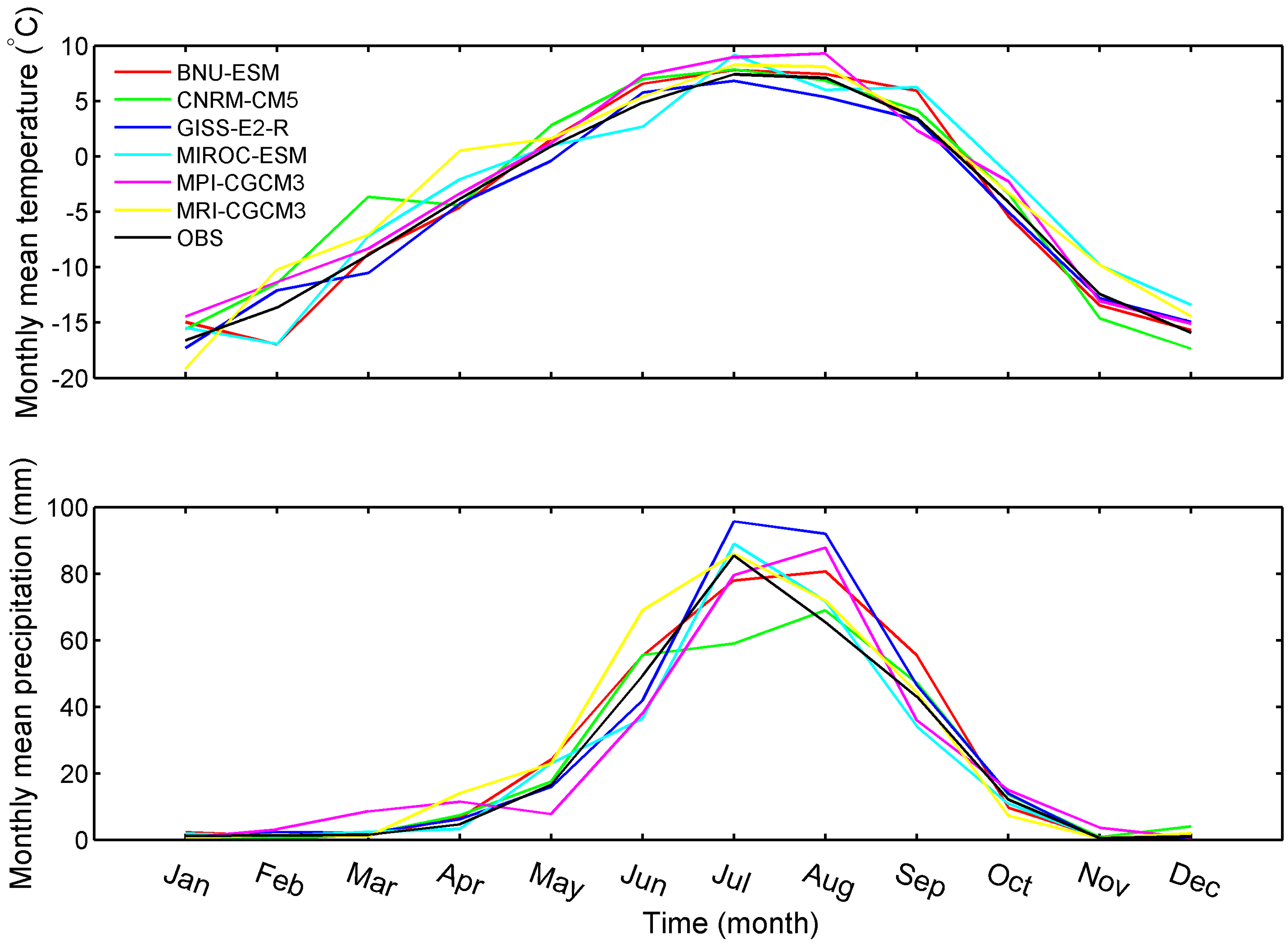
The evaluation of the ability of the GCMs to correctly represent the past plays an important role in this study. Three criteria, including monthly mean value, correlation coefficient (R) and root mean square error (RMSE), were applied to accomplish this work. The results of the three criteria were respectively shown in Figure 4 and

Table 4. R and RMSE values of the daily meteorology data from the six GCMs and meteorological station.

GCMs		BNU-ESM	CNRM-CM5	GISS-E2-R	MIROC-ESM	MPI-ESM-LR	MRI-CGCM3
R	Precipitation	0.71	0.68	0.66	0.72	0.82	0.77
	Temperature	0.82	0.85	0.86	0.92	0.93	0.85
RMSE	Precipitation	2.21	3.65	1.37	3.14	1.62	2.14
	Temperature	0.63	1.42	0.25	1.26	1.52	0.08

. For the monthly mean value of precipitation and temperature, the simulations of six GCMs showed acceptable results. For monthly temperature, the BNU-ESM projected the largest decrease (−3.29 °C) in February compares with the observed data while the MIROC-ESM gave the biggest increase (2.78 °C) in September. However, results were still acceptable while the changes of annual mean temperature of the six GCMs ranged from −0.32 °C to 1.07 °C. For the monthly mean precipitation, the change ratios ranged from −39.9% to 39.7%, however the annual mean value changed from −8.5% to 12.2% (June to October). For the R and RMSE, the six GCMs all showed satisfactory results. The R of precipitation ranged from 0.66 to 0.82 while that of temperature ranged from 0.82 to 0.93. The RMSE of precipitation ranged from 1.37 to 3.65 while that of temperature ranged from 0.08 to 1.52. In a word, based on the results of the three criteria, the six GCMs could correctly represent the past climate of this basin.

The generated daily data series were also tested using correlation coefficient (R) and root mean square error (RMSE) compared with the observed data. The result was shown in

Table 5. Validation results of the daily meteorology data generated by LARS-WG and the observed data using R and RMSE.

GCMs		BNU-ESM	CNRM-CM5	GISS-E2-R	MIROC-ESM	MPI-ESM-LR	MRI-CGCM3
R	Precipitation	0.85	0.82	0.81	0.86	0.92	0.89
	Temperature	0.87	0.89	0.88	0.95	0.96	0.97
RMSE	Precipitation	1.96	2.01	1.21	2.21	1.25	3.31
	Temperature	0.35	0.85	0.16	0.72	0.96	0.07

. For daily generated precipitation and temperature, the LARS-WG gave a satisfactory performance. The R of precipitation ranged from 0.81 to 0.92 while that of temperature ranged from 0.87 to 0.97. The RMSE of precipitation ranged from 1.25 to 3.31 while those of temperature ranged from 0.07 to 0.96. Generally, the LARS-WG displayed a good performance in generating daily meteorological data series.

3.2.1. Changes in Seasonal Mean Precipitation and Temperature

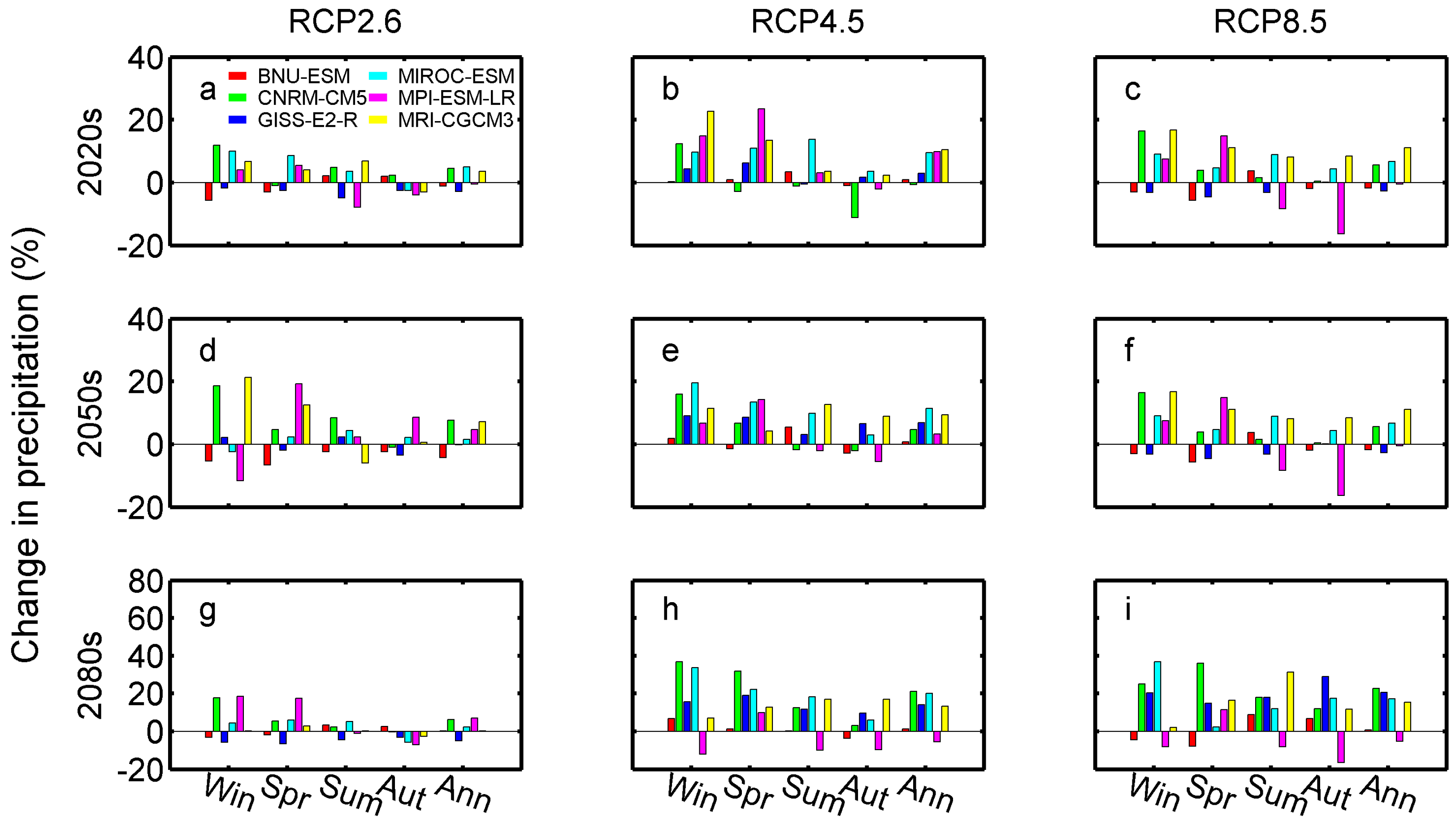
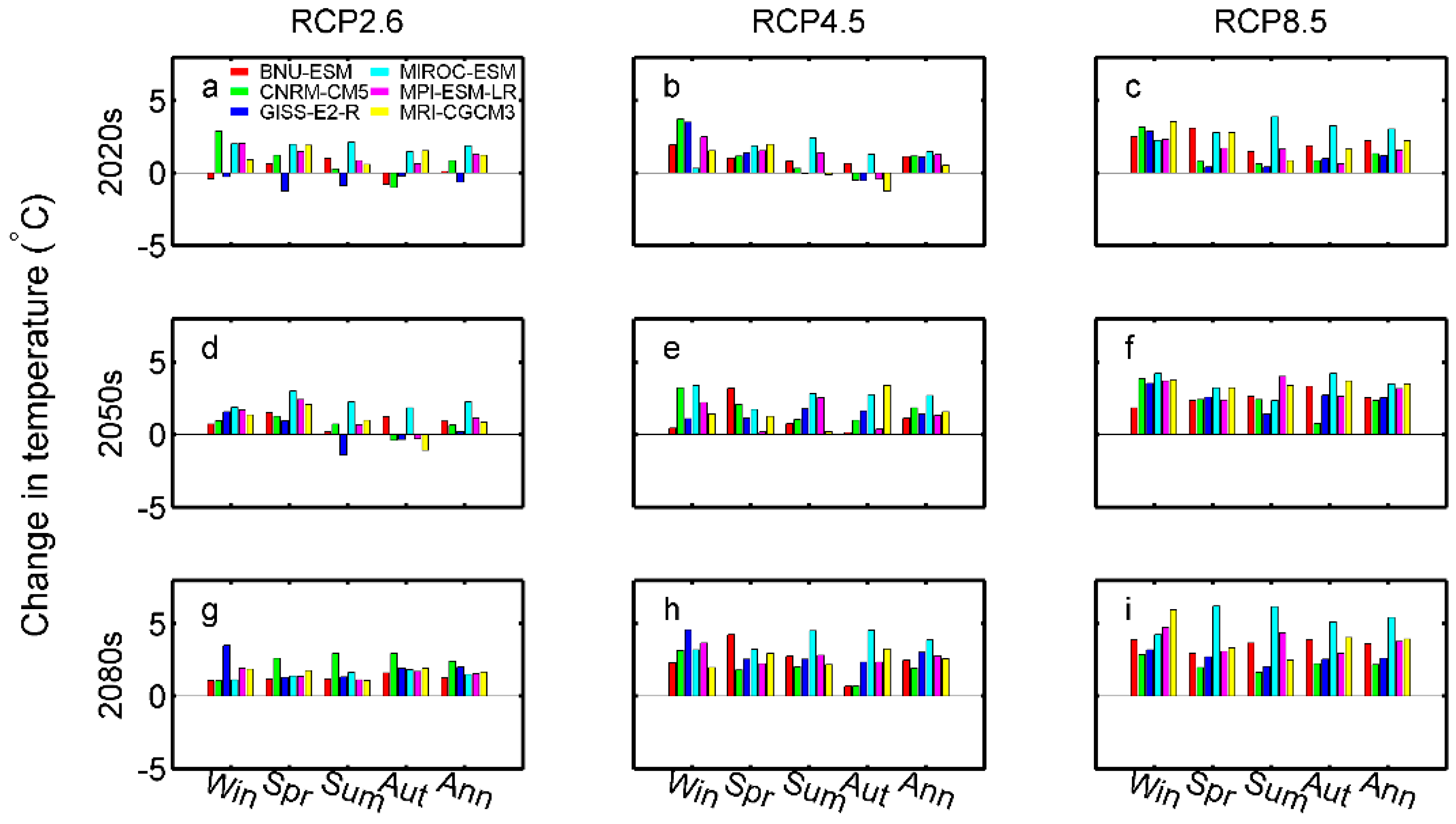
As the basin hydrology appeared to be closely related to the seasonal climatic conditions, climate change scenarios and the data analysis were performed on a seasonal basis for the future. Figure 5 and Figure 6 show changes in seasonal mean precipitation and temperature for the future periods under different RCPs, respectively. For the seasonal precipitation predictions, most of the GCMs gave increase projections for all the three future periods under different RCP scenarios. As shown in the figure, RCP8.5 always predicted a greater increase than the RCP4.5 and RCP2.6 scenarios in the annual mean precipitation. For the multi-GCMs, the average changes in the annual precipitation were 5.4%, 6.3% and 6.1% under RCP2.6, 8.3%, 12.6% and 15.9% under RCP4.5, and 7.1%, 16.1% and 28.4% under RCP8.5 for 2020s, 2050s and 2080s, respectively. These statistical results showed that in the future, the precipitation is predicted to be increased during the twenty-first century, especially in the 2080s. However, it also showed that there exists a big difference between GCMs and RCPs, which means that GCMs and RCPs can be considered the most important contributor of the uncertainty in these analyses.

From Figure 6, it was shown that the changes in temperature were not consistent with those of precipitation. The changes in temperature showed continuous growth. The average changes in annual mean temperature were 0.78 °C, 0.99 °C and 1.73 °C under RCP 2.6, 1.12 °C, 1.66 °C and 2.81 °C under RCP 4.5, 1.92 °C, 2.94 °C and 3.6 °C under RCP 8.5 for the 2020s, 2050s and 2080s, respectively.

For seasonal precipitation and temperature projected by different GCMs and RCPs, however, the difference in the seasonal values showed to be more significant than the annual changes. In general, this study area would be warmer and wetter in the future years.

3.2.2. Changes in Annual Mean Precipitation and Temperature

Table 6. Annual changes in Tasmin (°C) for the future periods (2020s, 2050s and 2080s) under RCPs (RCP 2.6, RCP 4.5 and RCP 8.5).

Periods	Annual Change in Tasmin (°C)
	BNU-ESM	CNRM-CM5	GISS-E2-R	MIROC-ESM	MPI-ESM-LR	MRI-CGCM3
RCP2.6
2020s	0.97	0.52	0.57	1.35	0.62	0.59
2050s	1.39	0.75	0.82	2.53	0.95	0.67
2080s	1.04	1.05	0.34	2.72	0.65	0.69
RCP4.5
2020s	1.20	0.39	1.12	1.93	0.65	0.67
2050s	1.98	1.36	2.32	3.62	1.53	1.63
2080s	2.46	1.78	2.77	4.66	1.98	1.92
RCP8.5
2020s	1.04	1.04	0.34	2.72	0.65	0.70
2050s	2.47	1.78	2.77	4.66	1.98	1.92
2080s	5.71	4.04	4.41	8.52	4.58	4.67

and

Table 7. Annual changes in tasmax (°C) for the future periods (2020s, 2050s and 2080s) under RCPs (RCP 2.6, RCP 4.5 and RCP 8.5).

Periods	Annual Change in Tasmax (°C)
	BNU-ESM	CNRM-CM5	GISS-E2-R	MIROC-ESM	MPI-ESM-LR	MRI-CGCM3
RCP2.6
2020s	1.01	0.41	0.55	1.31	0.66	0.59
2050s	1.58	0.74	0.84	2.23	1.01	0.71
2080s	1.23	0.96	0.58	2.45	0.54	0.90
RCP4.5
2020s	1.10	0.59	0.99	1.63	0.62	0.49
2050s	2.17	1.33	1.74	3.03	1.67	1.37
2080s	2.60	1.65	2.23	3.97	2.23	1.85
RCP8.5
2020s	1.23	0.96	0.58	2.45	0.54	0.90
2050s	2.59	1.65	2.22	3.96	2.23	1.85
2080s	5.33	3.15	4.03	7.09	5.01	3.91

respectively show the annual changes in the maximum and minimum temperature values (denoted as Tasmax and Tasmin, respectively) for the future prediction periods using six different GCMs under the three RCPs scenarios. In comparison to the precipitation, the trend change in temperature data showed to be more consistent. However, for the annual mean Tasmax and Tasmin under different RCPs, MIROC-ESM simulation scenarios always provided the largest increase in the future predictions.

For the Tasmin condition, the multi-GCMs ensemble, for the three time periods studied, provided increase in the magnitude from 0.77 °C to 1.08 °C under RCP2.6, 1.85 °C to 2.59 °C under RCP4.5, and 1.08 °C to 5.32 °C under RCP8.5 scenarios. For Tasmax, however, the results were relatively different compared with the Tasmin; under RCP2.6, the increase ranged from 0.75 °C to 1.11 °C, 1.18 °C to 2.42 °C under RCP4.5, and 1.11 °C to 4.75 °C under RCP8.5. Thus, temperature appeared to be an important factor affecting mostly on the evapotranspiration and the streamflow, suggesting that understanding the future change in trends for the Tasmax and the Tasmin values are critically important in evaluating the effects of the climate change on streamflow.

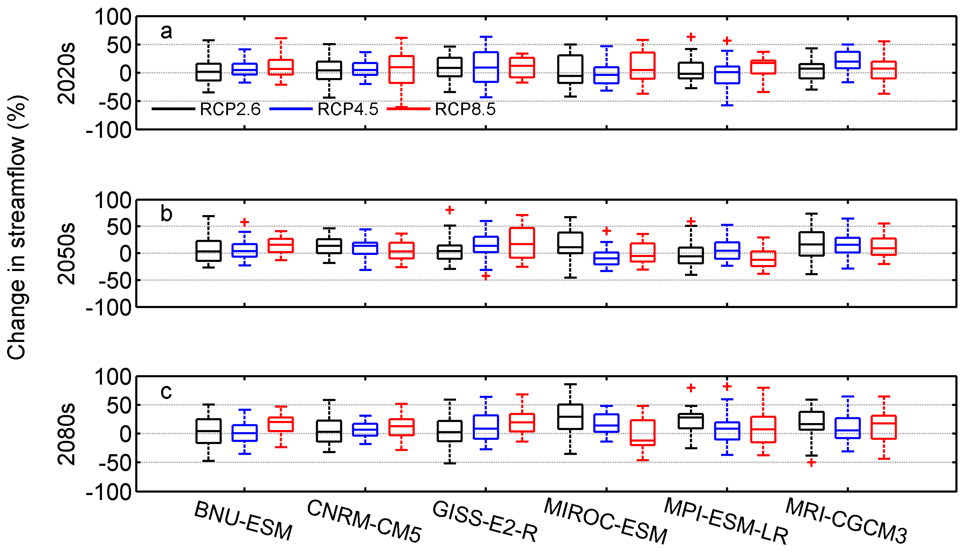
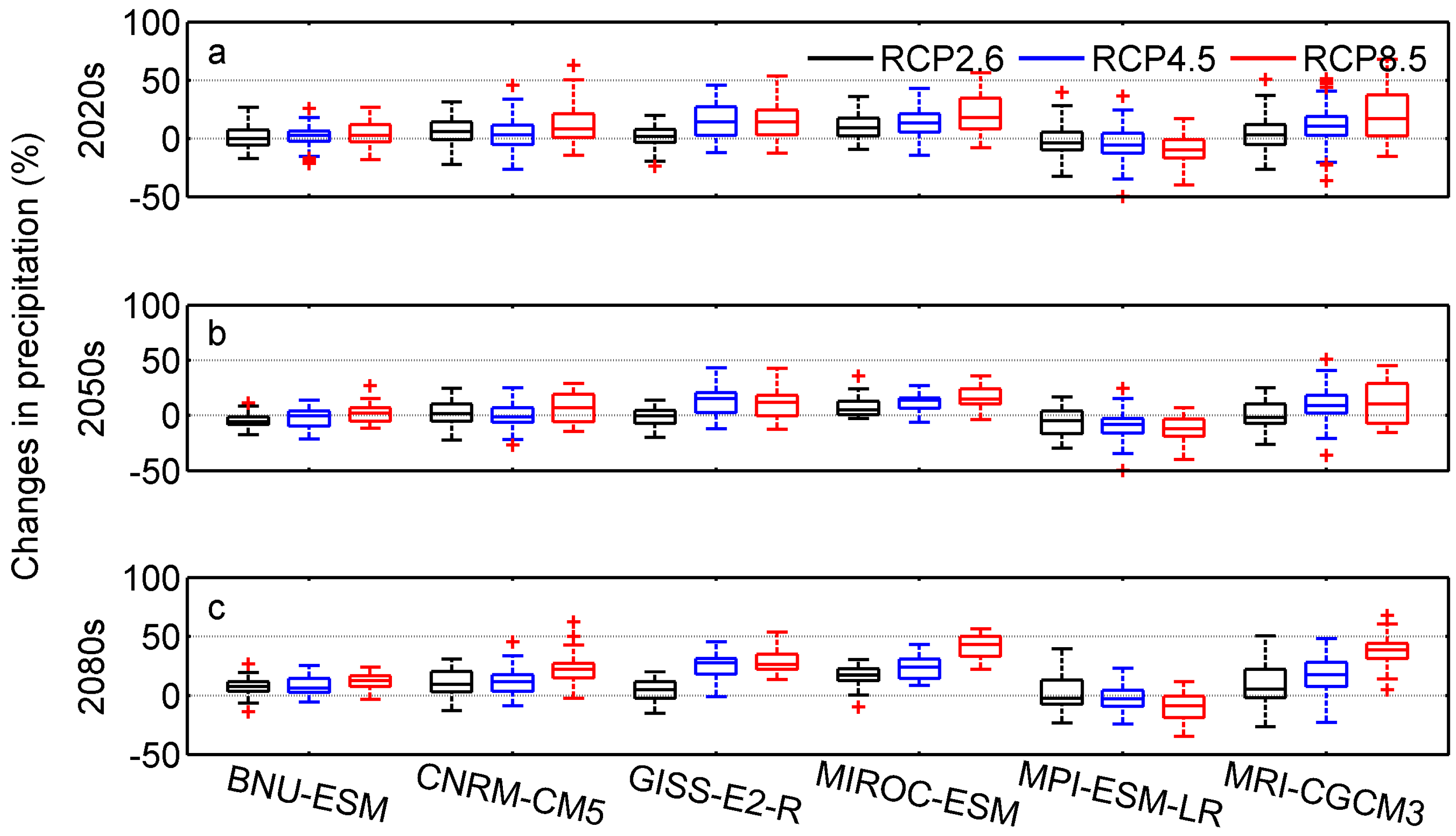
Figure 7 presents the change ratios for the simulated annual mean precipitation, compared to the control period through box plot, which could be applied to illustrate the dispersal of the data, by combination of GCMs and RCPs for the future prediction periods respectively.

For the 2020s, 2050s and 2080s, MPI-ESM-LR always provided the largest decreases in the median values. During all the three periods examined, nearly all GCMs used showed consistent results; the change ratios (in median) of precipitation under RCP8.5 gave the biggest value, while those of the RCP2.6 scenarios gave the lowest values. The only exception, however, was the MPI-ESM-LR; the change ratio in 2080s presented the largest decrease under RCP8.5. For the 2050s, the three models (BNU-ESM, CNRM-CM5, and GISS-E2-R) showed similar trends, compared with the 2080s, while the other GCMs (MIROC-ESM, MPI-ESM-LR, and MRI-CGCM3) projected slight changes among each others. In the 2020s analyses, MRI-CGCM3 and MPI-ESM-LR showed the biggest increase of 8.6% and 6.9% under RCP8.5 and RCP4.5, respectively, whereas in the 2050s predictions, the GISS-E2-R under RCP2.6 showed the biggest increase (17.8%) while the MPI-ESM-LR under RCP8.5 presented the biggest decrease (−8.0%). Meanwhile, in the 2080s, MIROC-ESM under RCP8.5 projected the largest increase (40.1%) and MPI-ESM-LR under RCP8.5 predicted the largest decrease (−13.8%). Data in Figure 8 also showed that the combinations of different GCMs and RCPs scenarios would lead to relatively a large amount of uncertainties in projecting the future climate change scenarios, and the uncertainty induced by GCM modeling itself is appeared to be the larger source, compared with the other sources of uncertainties.

3.2.3. Climate Change Impacts on Hydrology Simulations

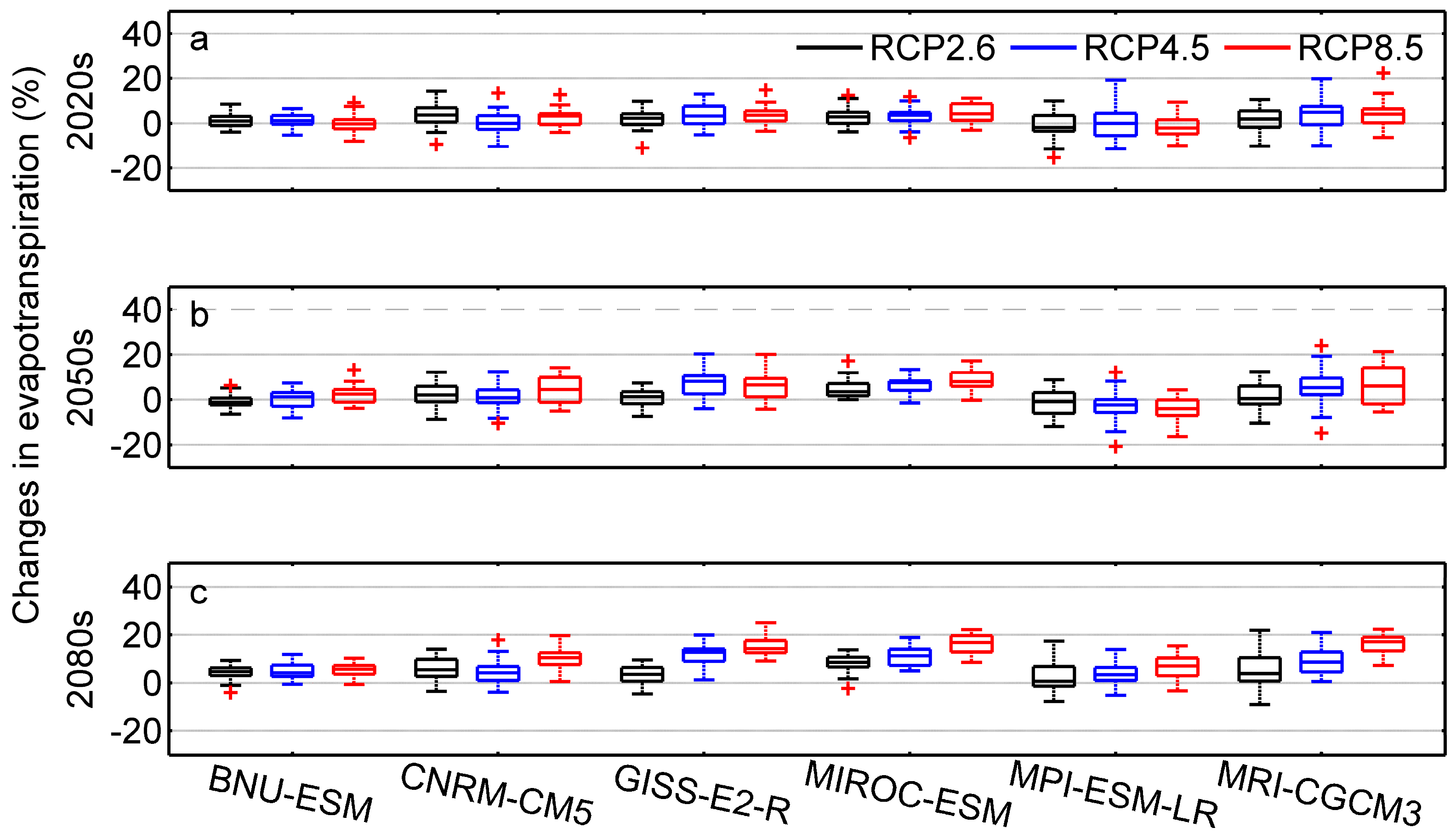
Figure 8 gives the simulation results on annual mean evapotranspiration simulated by the DHSVM under different GCMs and RCPs in the future time periods with box plot method. From the figure, it was shown that the changes of evapotranspiration had some similarities. During all the GCMs, the medians of MPI-ESM-LR under RCP 8.5 always gave the largest decrease ranging from −4.07% to −1.93% in the three future periods. In 2020s, MRI-CGCM3 represented the biggest increase in median (4.06%) under RCP 8.5. In 2050s, GISS-E2-R gave the largest increase in median (8.06%) under RCP 8.5, while MIROC-ESM showed the biggest increase (18.8%) under RCP 8.5. In 2020s, half GCMs (GISS-E2-R, MIROC-ESM and MRI-CGCM3) showed increase trend under the three RCPs. In 2050s, four GCMs (CNRM-CM5, GISS-E2-R, MIROC-ESM and MRI-CGCM3) gave the increase trend. While in 2080s all the GCMs, except MPI-ESM-LR, gave the increase trend in median. From the figure, it was also showed that the RCP 8.5 always gave the largest increase in median, while the RCP 2.6 always gave the smallest.

Figure 9 gives the probability density functions (PDFs) of the annual mean temperature, precipitation, and seasonal mean streamflow projected by the six GCMs used under the three RCPs scenarios for the future long-term prediction (2011–2100). Overall, the PDFs showed that nearly all six GCMs and the RCPs scenarios projected increase in both temperature and precipitation, suggesting that the future climate in this study area projected by GCMs under three RCPs will most likely expected to be warmer and wetter. It also showed that the increase in the magnitude of the change varied greatly between the different combinations of the GCMs and the three RCPs scenarios. More precisely, for the annual mean temperature, under RCP2.6, the MPI-ESM-LR predicted the largest increase (0.66 °C), whereas, GISS-E2-R predicted a decrease, the only decrease situation (−0.34 °C) among all the GCMs and RCPs examined, while under RCP4.5, MIROC-ESM provided the largest increase (4.78 °C) and BNU-ESM provided the smallest increase (1.39 °C), and under RCP8.5, the MIROC-ESM projected the largest increase (6.68 °C) and CNRM-CM5 projected the lowest increase (2.11 °C). For the annual precipitation, however, the GCMs behaved relatively consistent with temperature data. However, BNU-ESM always provided the smallest increase, ranged from 1.18% to 14.32% under all the three RCPs scenarios, while CNRM-CM5, MRI-CGCM3, and MIROC-ESM, provided the largest increase of nearly 36%, 72% and 65% under RCP2.6, RCP4.5, and RCP8.5 scenarios, respectively. For the seasonal mean streamflow, all GCMs under RCPs scenarios showed increased trend for the future predictions, however the mean streamflow showed greater differences, compared with other scenarios. Furthermore, the MRI-CGCM3 showed the largest increase in trend, ranged from 14.2% to 22.9% for the mean values of the seasonal streamflow data, while the MPI-ESM-LR analyses suggested the smallest increase in the trend, ranged from nearly 7.0% to 13.7%. Overall, for GISS-E2-R, MIROC-ESM-LR, and MRI-CGCM3, the change in the mean streamflow values under RCP8.5 were smaller than those under RCP2.6 and RCP4.5 scenarios.

Figure 10 presents the box plots of change ratios of the streamflow during the melt season (May–October) under the three RCPs scenarios in the three future prediction periods. As was shown in the figure, the change ratios for the future streamflow and precipitation showed slightly difference. For the 2020s, MRI-CGCM3 showed the largest increase (19.54%) under RCP4.5 scenario in the median case, whereas, MIROC-ESM showed the largest decrease (−5.7%) under RCP2.6 scenario. For the 2050s periods, GISS-E2-R and MPI-ESM-LR under RCP8.5 scenario projected the largest increase (16.74%) and decrease (−12.47%), respectively. For the 2080s period, MIROC-ESM provided the largest increase (28.98%) under RCP2.6 and MIROC-ESM gave the largest decrease (−12.23%) under RCP8.5. The mean values of the median projected by all GCMs and RCPs scenarios were 5.76%, 6.31%, and 10.64% for the three future periods, respectively. While the mean values of streamflow projected by all GCMs used and the RCPs scenarios were 6.6%, 8.19% and 11.76% for three future periods, respectively. These analyses clearly showed that the larger increase in the streamflow trend was in the 2080s, compared to the 2020s and the 2050s periods, which suggest that in the future prediction periods. Some researches pointed out that the annual rainfall and streamflow in the Upper Yangtze River basin (UYRB) is projected to decrease over the next 90 years [48,49], however there were some differences with this study in precipitation and streamflow. The main reason might be the increase of the evapotranspiration and the snowmelt in the source region of the Yangtze River.

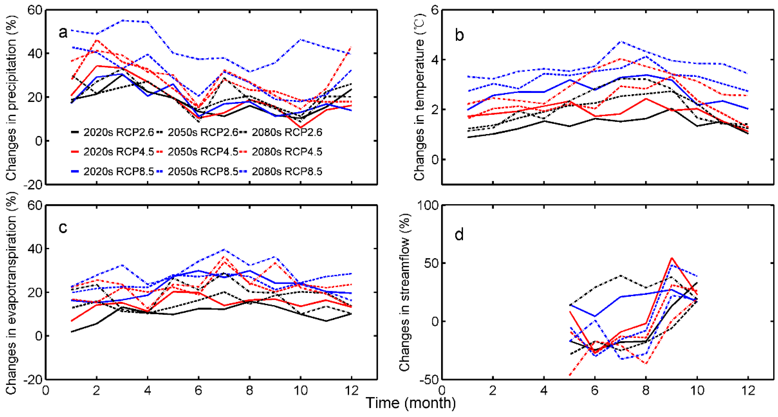
Figure 11 gives the changes ratios of monthly mean precipitation (a), temperature (b), evapotranspiration (c) and seasonal mean streamflow (d) for the future predictions under three RCPs. In this study, the multi-GCMs ensemble method was used to simulate the climate change scenarios which calculate the arithmetic mean value of the six GCMs outputs. In this study, the multi-GCM simulation was divided into nine scenarios (3 RCPs × 3 future periods).

For precipitation, however, the monthly changes showed interchangeable in the three future periods for the different scenarios. In all the scenarios tested, the trend of precipitation values in 2080s under RCP8.5 provided always the largest increase (31.52%–55.01%), while this trend in the precipitation in the 2020s showed the smallest increase. Furthermore, for all time period tested, multi-GCMs ensemble projected an increase in precipitation values, especially during the months of March, May and July. However in the Tuotuo River basin, summers have normally become much wetter as the precipitation distributions mostly concentrated during the months of May through August. The multi-GCMs ensemble results showed considerable differences between RCPs scenarios. The ensemble results also showed that the increase in the precipitation trend occurred mainly during the June and July time periods.

For temperature, the monthly results showed continuous change trends and all the predictions gave increase trends. During all the scenarios, the predictions in 2020s under RCP 2.6 always gave the smallest increase of variation (0.88 °C–2.03 °C), while those in 2080s under RCP 8.5 always gave the biggest increase (3.23 °C–4.73 °C). For all the months around the year, the biggest increase in temperature mainly occurred in July, August and September. In July, the increase in temperature ranged from 1.52 °C to 4.73 °C, in August, the increase ranged from 1.63 °C to 4.32 °C, while in September the increase ranged from 1.96 °C to 3.96 °C.

For evapotranspiration, it was shown in the figure that all the climate changes scenarios presented increase trends. During all the scenarios, the changes in 2080s under RCP 8.5 always showed the largest increase (16.25%–39.6%) while the changes in 2020s under RCP 2.6 always gave the smallest (1.86%–15.8%). It was also shown in the figure that the biggest increase mainly occurred in July (12.3%–39.6%), August (15.8%–32.25%) and September (13.6%–36.3%), which were similar to the changes of temperature.

Since the streamflow data were available only for the melting seasons (May to October) in Tuotuo River basin, the statistical comparison results of streamflow were also presented only for that specific time period. As indicted in Figure 11a, precipitation performed a substantial increase in winter season (December–February) more than other seasons, meaning that there would be more snow accumulation in winter. However, as energy in the arid zone is sufficient for forcing evapotranspiration [34], thus the increased precipitation would be mostly dissipated by increasing evapotranspiration and contribute to relatively little change of streamflow during this period in this study area.

Although the change in the monthly streamflow showed to be similar with the change in the monthly precipitation trend, there were negligible differences between them. Our analyses showed that among the future scenarios examined, the streamflow in 2020s under RCP2.6 and 2080s under RCP8.5 provided the smallest (4.36%) and biggest (41.52%) increases in trend, respectively, while the precipitation in 2080s under RCP8.5 always gave the biggest increase all year around. The main reason could most likely be due to the increase in temperature and the solar radiation during those time periods. This is primarily because the trend of temperature increase under RCP8.5 was more rapid than the same increase under RCP4.5 scenarios, suggesting that the increase in temperature corresponds to the increase in evapotranspiration that ultimately results in the decrease in streamflow. Thus, temperature can be considered as one of the key factors for analyzing the impacts of climate warming on the future prediction of the streamflow hydrology.

3.3. Uncertainty Analysis

The uncertainty in model simulations plays an important role for evaluating the effects of future climate change on the environment and should also be considered, especially in assessing that impact on the hydrology and water resources management of the Yangtze River source region. Uncertainties in this particular study can mainly be divided into three parts: (1) the uncertainty caused by the system errors of LARS-WG; (2) the uncertainty caused by the local hydrological model simulations; and (3) the uncertainty caused by the combinations of GCMs and RCPs examined. In this study, the part (3) of uncertainty source is discussed as follows.

There is no doubt that the uncertainty caused by GCMs is the main source of uncertainty for assessing the climate change impact on local water resource and hydrology. In this study, six GCMs were used to predict the future climate change scenarios and the results of the six GCMs showed large difference in precipitation. Under RCP 2.6, the changes in annual precipitation ranged from −7.6% to 17.31%; under RCP 4.5, the changes ranged from −8.63% to 27.68% while under RCP 8.5, the changes ranged from −12.17% to 43.01%. For annual mean temperature, there were relative small difference between different GCMs. The increase in the annual mean temperature given by the different GCMs were 0.46 °C to 2.58 °C under RCP 2.6, 0.44 °C to 4.31 °C under RCP 4.5 and 0.69 °C to 6.80 °C under RCP 8.5.

For the average predictions by a same GCM under different RCPs for the future periods, the changes in precipitation ranged from −5% to 25.3%, while the changes in temperature ranges from 0.69 °C to 2.58 °C. These results indicated that in the long time prediction, the uncertainty caused by RCPs is relatively smaller than that of GCMs.

Although only six GCMs were used in this research, some studies pointed out that these six GCMs were widely used and had a good performance in China [50,51,52]. In addition, this work involved downscaling of GCMs and hydrological simulation, the workload is relatively large. Thus, only six GCMs were used in this research. However, more kinds of GCMs would be considered and the differences of the GCMs would be analyzed in our future work.

The LARS-WG was primarily applied in this study to generate meteorological data. Different GCMs also expected to project different results both for the past and the future predictions. However, LARS-WG does not modify the future precipitation occurrence and its distribution that can be the major factor of uncertainty. In addition, the inverse distance weights method was also used to provide downscaling grids to stations that also can be an important factor. Therefore, LARS-WG can be considered as an inaccurate method in predicting extreme rainfall events for the short-term predictions, but would be apposite to be used for long-term predictions.

In addition, the uncertainty associated with the parameters of hydrological model could also influence the simulation results. Although DHSVM could interpolate the precipitation data in the plain region, the basin average precipitation data may not fully reflect the true situation in the mountainous areas. The coarse spatial resolution of 1 km for running DHSVM might bring about more errors for hydrological simulation especially in high elevation areas and the DHSVM could not simulate the peak streamflow very well. However, it is relatively not so important to focus on capturing the daily peak streamflow for studying the climate change impacts on hydrology in the long-time future projections. In addition, land use and soil types were assumed to be changeless with the climate change scenarios in this assessment. However, since the changes observed in soil and land use in this study area were relatively small in the past few decades, it can be considered as one of the sources of less uncertainty.

4. Conclusions

This paper focused on evaluating the response of local hydrology in the Tuotuo River basin to possible future climate changes using six GCMs coupled with three RCPs from IPCC AR5, the LARS-WG statistical downscaling method and a distributed hydrological soil vegetation model (DHSVM). Predictions provided by the six GCMs show that both temperature and precipitation will increase in the future periods. Generally, annual mean temperature was projected to increase for all scenarios, with changes ranging from 0.66 °C to 6.68 °C. In terms of annual mean precipitation, the change magnitude ranged from −1.18% to 66.14%. These findings reveal that the future climate of the Tuotuo River basin will be wetter and warmer.

The DHSVM was applied to assess the effects of the climate changes on the future evapotranspiration and stream hydrology. The change in evapotranspiration for the future periods ranges from −4.07% to 18.8%. In addition, the streamflow in this area will likely increase due to the increased in precipitation and the expected seasonal mean streamflow ranged from −0.52% to 22.58%. However, the change in the trend of streamflow was not consistent with that of increased in precipitation, because of the comprehensive effect of temperature and precipitation. Monthly streamflow showed to be increased from May to August and changed slightly during the other month. As was indicated in this research, the increase in precipitation was mainly concentrated during the wet seasons; for seasonal streamflow, that results in a more unequal distribution in the future, and needs to be paid more attentions in order to better manage the regional water resource availability.

As mentioned, uncertainties always exist in all processes involved in evaluating the climate change impacts on the environment. The main sources of the uncertainties were found to be caused by the different GCMs and RCPs used. This study attempted to quantify the uncertainties caused by the GCMs and RCPs. From the result, it was found that the uncertainties caused by RCPs were smaller than those caused by GCMs. However, there were still limitation of using only six models instead of all available CMIP5 models. The differences between models are the key factors, there were quite large discrepancies between different projected climate change scenarios based on GCMs outputs. As these GCMs were selected following other similar studies and different statistical indexes were applied to evaluate their applicability, these screening works guaranteed the reliability of these GCMs. Thus, although this research did not combine all the available GCMs and climate scenarios to study climate change impacts on the Tuotuo River basin, our feeling is that the six GCMs and three RCPs used were relatively adequate numbers to reasonably describe the climate change trend for this exceptional climatic region.

In future research, there is obviously a need for more downscaling methods, GCMs and RCPs to be employed to assess the effects of climate change scenarios on streamflow dynamics. The uncertainties that potentially can brought into this analyses by the local hydrological model should also been taken into account, however, it should be noted that their contributions are, in most cases, much smaller than those by GCMs. Due to the special geographical location of the Tibetan Plateau, our future study should focus more on the effects of climate change on the snow and glacier melting intensities as well as their contributions to the seasonal streamflow hydrology.

References

1. Li, Y.L.; Tao, H.; Yao, J.; Zhang, Q. Application of a distributed catchment model to investigate hydrological impacts of climate change within Poyang Lake Catchment (China). Hydrol. Res. 2016, 47, 120–135. [Google Scholar] [CrossRef]
2. Awan, U.K.; Liaqat, U.W.; Choi, M.; Ismaeel, A. A swat modeling approach to assess the impact of climate change on consumptive water use in Lower Chenab Canal area of Indus basin. Hydrol. Res. 2016, 47, 1025–1037. [Google Scholar] [CrossRef]
3. Srikanthan, R.; Mcmahon, T.A. Stochastic generation of annual, monthly and daily climate data: A review. Hydrol. Earth Syst. 2001, 5, 653–670. [Google Scholar] [CrossRef]
4. Xu, C.Y.; Singh, V.P. Review on regional water resources assessment models under stationary and changing climate. Water Resour. Manag. 2004, 18, 591–612. [Google Scholar] [CrossRef]
5. Solomon, S.; Qin, D.; Manning, M.; Chen, Z.; Marquis, M.; Averyt, K.B.; Tignor, M.; Miller, H.L. IPCC Fourth Assessment Report: Climate Change 2007—The Physical Science Basis (IPPC WGI AR4); Cambridge University Press: Cambridge, UK; New York, NY, USA, 2007. [Google Scholar]
6. Hartmann, C.L.A.D.L.; Brönnimann, S.; Dentener, F.J.; Dlugokencky, E.J.; Easterling, D.R.; Kaplan, A.; Soden, B.J. IPCC (2013), Climate Change 2013, in the Physical Science Basis, Working Group I Contribution to the Fifth Assessment Report of the Intergovernmental Panel on Climate Change; Cambridge University Press: Cambridge, UK, 2014. [Google Scholar]
7. Bowling, L.C.; Lettenmaier, D.P. The effects of forest roads and harvest on catchment hydrology in a mountainous maritime environment. In Land Use and Watersheds: Human Influence on Hydrology and Geomorphology in Urban and Forest Areas; American Geophysical Union: Washington, DC, USA, 2001. [Google Scholar]
8. Bueler, E.; Brown, J.; Lingle, C. Exact solutions to the thermomechanically coupled shallow-ice approximation: Effective tools for verification. J. Glaciol. 2007, 53, 499–516. [Google Scholar] [CrossRef]
9. Ligaray, M.; Kim, H.; Sthiannopkao, S.; Lee, S.; Cho, K.; Kim, J. Assessment on hydrologic response by climate change in the Chao Phraya River Basin, Thailand. Water 2015, 7, 6892–6909. [Google Scholar] [CrossRef]
10. Jin, H.; Zhu, Q.; Zhao, X.; Zhang, Y. Simulation and prediction of climate variability and assessment of the response of water resources in a typical watershed in China. Water 2016, 8, 490. [Google Scholar] [CrossRef]
11. Boé, J.; Terray, L.; Habets, F.; Martin, E. Statistical and dynamical downscaling of the Seine Basin climate for hydro-meteorological studies. Int. J. Climatol. 2007, 27, 1643–1655. [Google Scholar] [CrossRef]
12. Chen, J.; Brissette, F.P.; Leconte, R. Uncertainty of downscaling method in quantifying the impact of climate change on hydrology. J. Hydrol. 2011, 401, 190–202. [Google Scholar] [CrossRef]
13. Semenov, M.A.; Brooks, R.J.; Barrow, E.M.; Richardson, C.W. Comparison of the WGEN and LARS-WG stochastic weather generators for diverse climates. Clim. Res. 1998, 10, 95–107. [Google Scholar] [CrossRef]
14. Fowler, H.J.; Blenkinsop, S.; Tebaldi, C. Linking climate change modelling to impacts studies: Recent advances in downscaling techniques for hydrological modelling. Int. J. Climatol. 2007, 27, 1547–1578. [Google Scholar] [CrossRef]
15. Luo, Q.; Wen, L.; Mcgregor, J.L.; Timbal, B. A comparison of downscaling techniques in the projection of local climate change and wheat yields. Clim. Chang. 2013, 118, 249–261. [Google Scholar] [CrossRef]
16. Etemadi, H.; Samadi, S.; Sharifikia, M. Uncertainty analysis of statistical downscaling models using general circulation model over an international wetland. Clim. Dyn. 2014, 42, 2899–2920. [Google Scholar] [CrossRef]
17. Duan, K.; Mei, Y. Comparison of meteorological, hydrological and agricultural drought responses to climate change and uncertainty assessment. Water Resour. Manag. 2014, 28, 5039–5054. [Google Scholar] [CrossRef]
18. Zhuang, X.W.; Li, Y.P.; Huang, G.H.; Liu, J. Assessment of climate change impacts on watershed in cold-arid region: An integrated multi-GCM-based stochastic weather generator and stepwise cluster analysis method. Clim. Dyn. 2015, 47, 1–19. [Google Scholar] [CrossRef]
19. Yang, K.; Wu, H.; Qin, J.; Lin, C.; Tang, W.; Chen, Y. Recent climate changes over the Tibetan Plateau and their impacts on energy and water cycle: A review. Glob. Planet. Chang. 2014, 112, 79–91. [Google Scholar] [CrossRef]
20. Gao, H.; He, X.; Ye, B.; Pu, J. Modeling the runoff and glacier mass balance in a small watershed on the central Tibetan Plateau, China, from 1955 to 2008. Hydrol. Process. 2012, 26, 1593–1603. [Google Scholar] [CrossRef]
21. Li, L.; Hao, Z.C.; Wang, J.H.; Wang, Z.H.; Yu, Z.B. Impact of future climate change on runoff in the head region of the Yellow River. J. Hydrol. Eng. 2008, 13, 347–354. [Google Scholar] [CrossRef]
22. Chen, X.; You, Q.; Sielmann, F.; Ruan, N. Climate change scenarios for Tibetan Plateau summer precipitation based on canonical correlation analysis. Int. J. Climatol. 2016, 36, 2173–2188. [Google Scholar] [CrossRef]
23. Shi, P.; Duan, K.; Liu, Q.; Yang, J.; Zhang, X.; Sun, J. Response of Xiao Dongkemadi Glacier in the central Tibetan Plateau to the current climate change and future scenarios by 2050. J. Mt. Sci. 2016, 13, 13–28. [Google Scholar] [CrossRef]
24. Yong, Z.; Liu, S.; Xu, J.; Shangguan, D. Glacier change and glacier runoff variation in the Tuotuo River Basin, the source region of Yangtze River in Western China. Environ. Geol. 2008, 56, 59–68. [Google Scholar]
25. Yao, Z.; Liu, Z.; Huang, H.; Liu, G.; Wu, S. Statistical estimation of the impacts of glaciers and climate change on river runoff in the headwaters of the Yangtze River. Quat. Int. 2014, 336, 89–97. [Google Scholar] [CrossRef]
26. Guo, W.; Xu, J.; Liu, S.; Shangguan, D.; Wu, L.; Yao, X.; Zhao, J.; Liu, Q.; Jiang, Z.; Li, P.; et al. The Second Glacier Inventory Dataset of China, version 1.0; Cold and Arid Regions Science Data Center: Lanzhou, China, 2014. [Google Scholar]
27. Taylor, K.E.; Stouffer, R.J.; Meehl, G.A. An overview of CMIP5 and the experiment design. Bull. Am. Meteorol. Soc. 2011, 93, 485–498. [Google Scholar] [CrossRef]
28. Vuuren, D.P.V.; Edmonds, J.; Kainuma, M.; Riahi, K.; Thomson, A.; Hibbard, K.; Hurtt, G.C.; Kram, T.; Krey, V.; Lamarque, J.F. The representative concentration pathways: An overview. Clim. Chang. 2011, 109, 5–31. [Google Scholar] [CrossRef]
29. Naz, B.S.; Kao, S.C.; Ashfaq, M.; Rastogi, D.; Mei, R.; Bowling, L.C. Regional hydrologic response to climate change in the conterminous United States using high-resolution hydroclimate simulations. Glob. Planet. Chang. 2016, 143, 100–117. [Google Scholar] [CrossRef]
30. Beecham, S.; Rashid, M.; Chowdhury, R.K. Statistical downscaling of multi-site daily rainfall in a south Australian catchment using a generalized linear model. Int. J. Climatol. 2014, 34, 3654–3670. [Google Scholar] [CrossRef]
31. Basheer, A.K.; Lu, H.; Omer, A.; Ali, A.B.; Abdelgader, A.M.S. Impacts of climate change under CMIP5 RCP scenarios on the streamflow in the Dinder River and ecosystem habitats in Dinder National Park, Sudan. Hydrol. Earth Syst. Sci. Discuss. 2015, 12, 10157–10195. [Google Scholar] [CrossRef]
32. Khadka, D.; Babel, M.S.; Shrestha, S.; Tripathi, N.K. Climate change impact on glacier and snow melt and runoff in Tamakoshi Basin in the Hindu Kush Himalayan (HKH) Region. J. Hydrol. 2014, 511, 49–60. [Google Scholar] [CrossRef]
33. Su, F.; Zhang, L.; Ou, T.; Chen, D.; Yao, T.; Tong, K.; Qi, Y. Hydrological response to future climate changes for the major upstream river basins in the Tibetan Plateau. Glob. Planet. Chang. 2015, 136, 82–95. [Google Scholar] [CrossRef]
34. Zhang, Y.; Su, F.; Hao, Z.; Xu, C.; Yu, Z.; Wang, L.; Tong, K. Impact of projected climate change on the hydrology in the headwaters of the Yellow River Basin. Hydrol. Process. 2015, 29, 4379–4397. [Google Scholar] [CrossRef]
35. Ouyang, F.; Zhu, Y.; Fu, G.; Lü, H.; Zhang, A.; Yu, Z.; Chen, X. Impacts of climate change under CMIP5 RCP scenarios on streamflow in the Huangnizhuang catchment. Stoch. Environ. Res. Risk Assess. 2015, 29, 1781–1795. [Google Scholar] [CrossRef]
36. Semenov, M.A.; Barrow, E.M. Use of a stochastic weather generator in the development of climate change scenarios. Clim. Chang. 1997, 35, 397–414. [Google Scholar] [CrossRef]
37. Toews, M.W.; Allen, D.M. Evaluating different gcms for predicting spatial recharge in an irrigated arid region. J. Hydrol. 2009, 374, 265–281. [Google Scholar] [CrossRef]
38. Wigmosta, M.S.; Vail, L.W.; Lettenmaier, D.P. A distributed hydrology-vegetation model for complex terrain. Water Resour. Res. 1994, 30, 1665–1679. [Google Scholar] [CrossRef]
39. Wallis, T.W.R.; Griffiths, J.F. An assessment of the weather generator (WXGEN) used in the erosion/productivity impact calculator (EPIC). Agric. For. Meteorol. 1995, 73, 115–133. [Google Scholar] [CrossRef]
40. Bae, D.H.; Jung, I.W.; Lettenmaier, D.P. Hydrologic uncertainties in climate change from IPCC AR4 GCM simulations of the Chungju Basin, Korea. J. Hydrol. 2011, 401, 90–105. [Google Scholar] [CrossRef]
41. Nash, J.E.; Sutcliffe, J.V. River flow forecasting through conceptual models part I—A discussion of principles. J. Hydrol. 1970, 10, 282–290. [Google Scholar] [CrossRef]
42. Gupta, H.V.; Kling, H.; Yilmaz, K.K.; Martinez, G.F. Decomposition of the mean squared error and NSE performance criteria: Implications for improving hydrological modelling. J. Hydrol. 2009, 377, 80–91. [Google Scholar] [CrossRef]
43. Magnusson, J.; Wever, N.; Essery, R.; Helbig, N.; Winstral, A.; Jonas, T. Evaluating snow models with varying process representations for hydrological applications. Water Resour. Res. 2015, 51, 2707–2723. [Google Scholar] [CrossRef]
44. Nicolle, P.; Pushpalatha, R.; Perrin, C.; François, D.; Thiéry, D.; Mathevet, T.; Lay, M.L.; Besson, F.; Soubeyroux, J.M.; Viel, C. Benchmarking hydrological models for low-flow simulation and forecasting on French catchments. Hydrol. Earth Syst. Sci. 2014, 18, 2829–2857. [Google Scholar] [CrossRef] [Green Version]
45. Dick, J.J.; Tetzlaff, D.; Birkel, C.; Soulsby, C. Modelling landscape controls on dissolved organic carbon sources and fluxes to streams. Biogeochemistry 2015, 122, 361–374. [Google Scholar] [CrossRef] [Green Version]
46. Zhao, Q.; Ye, B.; Ding, Y.; Zhang, S.; Yi, S.; Wang, J.; Shangguan, D.; Zhao, C.; Han, H. Coupling a glacier melt model to the variable infiltration capacity (VIC) model for hydrological modeling in North-Western China. Environ. Earth Sci. 2013, 68, 87–101. [Google Scholar] [CrossRef]
47. Naz, B.S.; Frans, C.D.; Clarke, G.K.C.; Burns, P.; Lettenmaier, D.P. Modeling the effect of glacier recession on streamflow response using a coupled glacio-hydrological model. Hydrol. Earth Syst. Sci. 2014, 18, 787–802. [Google Scholar] [CrossRef] [Green Version]
48. Guo, J.; Chen, H.; Xu, C.Y.; Guo, S.; Guo, J. Prediction of variability of precipitation in the Yangtze River Basin under the climate change conditions based on automated statistical downscaling. Stoch. Environ. Res. Risk Assess. 2012, 26, 157–176. [Google Scholar] [CrossRef]
49. Sun, J.; Lei, X.; Tian, Y.; Liao, W.; Wang, Y. Hydrological impacts of climate change in the upper reaches of the Yangtze River Basin. Quat. Int. 2013, 304, 62–74. [Google Scholar] [CrossRef]
50. You, Q.; Fraedrich, K.; Sielmann, F.; Min, J.; Kang, S.; Ji, Z.; Zhu, X.; Ren, G. Present and projected degree days in China from observation, reanalysis and simulations. Clim. Dyn. 2013, 43, 1449–1462. [Google Scholar] [CrossRef]
51. Chen, L.; Frauenfeld, O.W. Surface air temperature changes over the twentieth and twenty-first centuries in China simulated by 20 CMIP5 models. J. Clim. 2014, 27, 3920–3937. [Google Scholar] [CrossRef]
52. Li, J.; Mao, J. Changes in the boreal summer intraseasonal oscillation projected by the CNRM-CM5 model under the RCP 8.5 scenario. Clim. Dyn. 2016, 107, 1–24. [Google Scholar] [CrossRef]
Figure 1. Location of the Tuotuo River basin.
Water 09 00070 g001
Figure 2. Soil types and land covers over the study area.
Water 09 00070 g002
Figure 3. The simulation results for calibration and validation periods.
Water 09 00070 g003
Figure 4. Monthly mean of the past simulation.
Water 09 00070 g004
Figure 5. Changes in seasonal precipitation (%) in the future periods (2020s, 2050s and 2080s) under RCP 2.6, RCP 4.5 and RCP 8.5: (a) 2020s under RCP2.6; (b) 2020s under RCP4.5; (c) 2020s under RCP8.5; (d) 2050s under RCP 2.6; (e) 2050s under RCP4.5; (f) 2050s under RCP8.5; (g) 2080s under RCP2.6; (h) 2080s under RCP4.5; (i) 2080s under RCP8.5.
Water 09 00070 g005
Figure 6. Changes in seasonal temperature (°C) in the future periods (2020s, 2050s and 2080s) under RCP 2.6, RCP 4.5 and RCP 8.5: (a) 2020s under RCP2.6; (b) 2020s under RCP4.5; (c) 2020s under RCP8.5; (d) 2050s under RCP 2.6; (e) 2050s under RCP4.5; (f) 2050s under RCP8.5; (g) 2080s under RCP2.6; (h) 2080s under RCP4.5; (i) 2080s under RCP8.5.
Water 09 00070 g006
Figure 7. Box plots of change ratios in annual precipitation (%) in the future periods ((a) 2020s, (b) 2050s and (c) 2080s) under RCPs (RCP2.6, RCP4.5 and RCP8.5).
Water 09 00070 g007
Figure 8. Box plots of change ratios in annual evapotranspiration (%) in the future periods ((a) 2020s, (b) 2050s and (c) 2080s) under RCPs (RCP2.6, RCP4.5 and RCP8.5).
Water 09 00070 g008
Figure 9. Box plots of change ratios in seasonal streamflow (%) in the future periods ((a) 2020s, (b) 2050s and (c) 2080s) under RCPs (RCP2.6, RCP4.5 and RCP8.5).
Water 09 00070 g009
Figure 10. Probability density functions plots of annual mean temperature, precipitation and seasonal mean streamflow in future (2011–2100) under three RCPs ((a,d,g) RCP2.6, (b,e,f) RCP4.5 and (c,f,i) RCP8.5).
Water 09 00070 g010
Figure 11. Changes in monthly precipitation (a), temperature (b), evapotranspiration (c) and streamflow (d) under RCPs for the future periods.
Water 09 00070 g011