Long-Term Streamflow Forecasting Based on Relevance Vector Machine Model

Abstract

Long-term streamflow forecasting is crucial to reservoir scheduling and water resources management. However, due to the complexity of internally physical mechanisms in streamflow process and the influence of many random factors, long-term streamflow forecasting is a difficult issue. In the article, we mainly investigated the ability of the Relevance Vector Machine (RVM) model and its applicability for long-term streamflow forecasting. We chose the Dahuofang (DHF) Reservoir in Northern China and the Danjiangkou (DJK) Reservoir in Central China as the study sites, and selected the 500 hpa geopotential height in the northern hemisphere and the sea surface temperatures in the North Pacific as the predictor factors of the RVM model and the Support Vector Machine (SVM) model, and then conducted annual streamflow forecasting. Results indicate that forecasting results in the DHF Reservoir is much better than that in the DJK Reservoir when using SVM, because streamflow process in the latter basin has a magnitude bigger than 1000 m³/s. Comparatively, accurate forecasting results in both the two basins can be gotten using the RVM model, with the Nash Sutcliffe efficiency coefficient bigger than 0.7, and they are much better than those gotten from the SVM model. As a result, the RVM model can be an effective approach for long-term streamflow forecasting, and it also has a wide applicability for the streamflow process with a discharge magnitude from dozen to thousand cubic meter per second.

1. Introduction

Conducting streamflow forecasting, especially long-term streamflow forecasting at monthly, annual, inter-annual or even decadal scales, is an important precondition for reservoir scheduling, water resources management, flood control and many other practical water activities [1,2]. However, it is a difficult task in practice due to the stochastic and nonlinear characteristics of streamflow process at multi-time scales [3,4]. During the recent decades, a large number of methods have been developed and improved for the streamflow forecasting. They can be generally divided into two types: process-driven methods and data-driven methods [5]. The former are based on mathematical simulation of streamflow process and the internally physical mechanisms that contribute to the hydrological cycle [6]. Process-driven methods usually require a large number of data inputs and parameter calibration. Comparatively, data-driven methods usually identify and describe the correlation between inputs and outputs, without considering the physical mechanisms of hydrological process in a watershed, and thus they have two advantages of low quantitative demand of data and simple formulation.

Owing to the complexity of physical mechanism in streamflow process and the influences of many random factors, the results gotten from process-driven methods cannot meet practical needs enough in some situations, especially in those data-ungauged basins. Comparatively, data-driven methods are an effective alternative, and they have been more widely used for long-term streamflow forecasting [7]. Data-driven methods generally include times series analysis-based and artificial intelligence (AI)-based methods [8,9,10,11]. They are simple and can be easily implemented, and so play an important role in hydrology research. However, the data should be stationary and follow normal distribution when using traditional times series analysis-based methods, which perform poorly in predicting extreme (both peak and small) streamflow values. Recently, AI technique has become increasingly popular in hydrology. Artificial neural networks (ANNs) model, one type of AI models, has gained more popularity for hydrological forecasting [12,13]. An extensive review about the model type can be found in the references [7,8]. However, a hard problem for ANNs is underfitting or overfitting [14], which would influence their fault-tolerant capability.

Another type of AI-based methods, called Support Vector Machine (SVM), has attracted the concerns from many researchers [15,16,17,18,19,20]. SVM is based on the structural risk minimization (SRM) principle and is an approximation implementation of SRM, with a good generalization capability [15]. It is considered as a kernel-based learning system rooted in the statistical learning theory, and has been applied widely for streamflow forecasting. For example, Asefa et al. used SVM to forecast flows at seasonal and hourly scales in the Sevier River Basin [17]; Lu et al. indicated a superior SVM performance over ANN in forecasting annual runoff [18]; and Li et al. predicted runoff by coupling SVM with the chaos analysis [19]. An improved SVM model, called Relevance Vector Machine (RVM), was proposed by Tipping [21,22]. It has the identical functional form as SVM [23,24]. RVM introduces a general Bayesian framework for obtaining sparse solution, and can derive accurate prediction models which typically utilize fewer basis functions than SVM; further, it can offer a number of additional advantages such as the benefit of probabilistic prediction, automatic estimation of parameters, and the facility to utilize arbitrary basis functions. The RVM model has been successfully applied for the pattern recognition and regression in different fields, including power load forecast and quality inspection [25]. However, there are relatively fewer applications of RVM in hydrology compared with other AI-based methods.

The objective of this study is therefore to investigate the performance of the RVM model in long-term streamflow forecasting, and further demonstrate its applicability for different basins. To achieve the goal, we chose the Dahuofang (DHF) Reservoir in North China and the Danjiangkou (DJK) Reservoir in Central China, which have obviously different underlying surface conditions and climate conditions, as the study areas and conduct long-term streamflow forecasting. Before it is feasible, how to identify proper physical factors which influence runoff is an important task for developing reliable model. Many researchers have investigated the statistical relationship between hydrological variables and ocean-atmospheric signals, such as the El Nino-Southern Oscillation, sea surface temperature (SST) and others [9,26,27,28,29,30,31,32]. Because ocean-atmospheric signals have time-lag effect on hydrological variables, models based on these factors could extend the forecasting period. Here the ocean-atmospheric signals, including the atmospheric circulation patterns of 500 hpa geopotential height in the northern hemisphere and the sea surface temperatures (SSTs) in the North Pacific, are used as the predictor factors, and the RVM model is applied for annual streamflow forecasting in the DHF and DJK basins.

2. The RVM Model

A brief description of the RVM model is provided here. The idea of the learning machine was first proposed by Turing [33]; after then, Vapnik discussed the feature of learning machine and proposed SVM, based on the statistical learning [16]. Tipping put forward a Sparse Bayesian learning model called RVM [21]. It can give more accurate prediction and utilize much fewer basis functions than SVM; further, the RVM model can describe the distribution function of the predicting variable under the Bayesian probabilistic framework.

Given a set of training data ${\left\{x_n,t_n\right\}}_{n=1}^N$, where x_n is the input vector and t_n is the target vector with the total number of N, the output for the RVM model is given as:

$$t_n=y(w_n;w)+{\epsilon }_n\text{ with }y(x;\omega )={\displaystyle \sum _{i=1}^N{\omega }_{i}K(x,x_i)+{\omega }_0}$$

(1)

where $w={({\omega }_1,{\omega }_2,\cdots ,{\omega }_N)}^T$ are parameters, ε_n are independent samples following a Gaussian distribution ${\epsilon }_n~N(0,{\sigma }^2)$, and $K(x,x_i)$ is a kernel function. Here the Gauss radial basis function $G(x,x_i)=\exp (-\frac{{\Vert x-x_i\Vert }^2}{{\sigma }^2})$, which has low complexity and has been used widely, is used as the kernel for the study of two cases. The parameters are estimated by the maximum likelihood method:

$$p(t|w,{\sigma }^2)={(2\pi {\sigma }^2)}^{-N/2}\exp \left\{-\frac{1}{2{\sigma }^2}{\left|t-\varphi w\right|}^2\right\}$$

(2)

where $t={(t_1\cdots t_N)}^T$, $w={({\omega }_0\cdots {\omega }_N)}^T$; $\varphi ={[\phi (x_1),\phi (x_2),\cdots ,\phi (x_N)]}^T$ is a $N\times (N+1)$ designed matrix, with $\phi (x_N)={[1,K(x_n,x_1),K(x_n,x_2),\cdots ,K(x_n,x_1)]}^T$. All parameters in Equation (2) compose a vector of hyperparameters, with the total number of N + 1. Following the general practice, we chose the Gamma distribution as the hyperpriors of all parameters α:

$$Gamma(\alpha |a,b)=\mathsf{\Gamma }{(a)}^{-1}{b}^a{\alpha }^{a-1}{e}^{-b\alpha }$$

(3)

with $\mathsf{\Gamma }(a)={\displaystyle {\int }_0^{\infty }{t}^{a-1}{e}^{-t}dt}$. In order to gain the same hyperpriors, here we fix the intimal values of those parameters in Equation (3) as 0.001. Then, following the Bayesian inference the posterior of all parameters can be described as:

$$p(\omega ,\alpha ,{\sigma }^2|t)=\frac{p(t|\omega ,\alpha ,{\sigma }^2)p(\omega ,\alpha ,{\sigma }^2)}{p(t)}$$

(4)

For a new test point $x_{*}$, predictions can be made at the corresponding target $t_{*}$ in terms of the predictive distribution:

$$p(t_{*}|t)={\displaystyle \int p(t_{*}|w,\alpha ,{\sigma }^2)}p(w,\alpha ,{\sigma }^2|t)dwd\alpha d{\sigma }^2$$

(5)

After determining the optimal hyperparameters ${\alpha }_{MP}$ and ${\sigma }_{MP}^2$, we can describe the predictive distribution as:

$$p(t_{*}|t,{\alpha }_{MP},{\sigma }_{MP}^2)={\displaystyle \int p(t_{*}|w,\alpha ,{\sigma }_{MP}^2)}p(w|t,{\alpha }_{MP},{\sigma }_{MP}^2)dw$$

(6)

Because both terms in the above integrand function are the Gaussian distribution, they can also be expressed as:

$$p(t_{*}|t,{\alpha }_{MP},{\sigma }_{MP}^2)=N(t_{*}|y_{*},{\sigma }_{*}^2)$$

(7)

with $y_{*}={\mu }^T\varphi (x_{*})$ and ${\sigma }_{*}^2={\sigma }_{MP}^2+\varphi {(x_{*})}^T\mathsf{\Sigma }\varphi (x_{*})$. Finally, the predictive mean is $y(x_{*};\mu )$.

More detailed description of the RVM model can be found in [21,22]. The forecasting process of hydrological variables by RVM can also be found in the flow chart in Figure 1.

3. Materials

3.1. Study Area

The Dahuofang (DHF) Reservoir and the Danjiangkou (DJK) Reservoir are chosen as the study sites (Figure 2), with an average annual precipitation of 800 mm and 870 mm respectively. The DHF Reservoir is located in the mid reaches of the Hun River, China, with a basin area of 5437 km² and a water capacity of 2.27 billion m³. It supplies water to the Shenyang and Fushun cities, provides water resources for the agriculture in the Liaoning Province, and protects the downstream regions from flood disasters. The DJK Reservoir, as a tributary of the Yangtze River, is located in the upper reaches of the Hanjiang River, with a basin area of 96,217 km² and a water capacity of 30 billion m³. The DJK Reservoir aims at flood control, power generation, irrigation and shipping functions. Because the two reservoirs were designed as annual regulation, annual streamflow forecasting has socioeconomic significance for local regions.

3.2. Data Sets

The data sets used for long-term streamflow forecasting include the oceanic-atmospheric signals and the naturalized annual streamflow data at the DHF and DJK Reservoir. The annual streamflow data were measured from 1962 to 2006 in the DHF Reservoir, and those were measured from 1957 to 2006 in the DJK Reservoir. These runoff data were gotten from the Chinese Hydrological Yearbook.

The oceanic-atmospheric signals include the atmospheric circulation patterns of 500 hpa geopotential height (Z₅₀₀) in the northern hemisphere and SSTs in the North Pacific. The data of Z₅₀₀ in the northern hemisphere are a product of the NCEP/NCAR reanalysis 40-year Project and were obtained from the NOAA Physical Sciences Center (http://www.cdc.noaa.-gov/cgi-bin/Composites/printpage.pl). The data of the Z₅₀₀ index are given on a 2.5° by 2.5° latitude and longitude grid, and are available from 1948 to present. The region with the latitude 0° N–90° N and longitude 0° W–2.5° W was considered for the study. The data of SSTs in the North Pacific were obtained from the National Climatic Data Center (http://www.cdc.noaa.gov/cdc/data.noaa.ersst.html). The SSTs data consist of average monthly values for a 2° by 2° grid. The extended reconstructed global SSTs were based on the comprehensive ocean-atmosphere data set from 1854 to present. The region of the North Pacific Ocean (120° E–80° W and 10° S–50° N) was also considered for the study.

In the modelling practice, both the Z₅₀₀ and SSTs are used as the predictor factors, that is, the input data of model; the streamflow data at each reservoir are the output data of model.

4. Results and Discussion

4.1. Selection of Predictor Factors

How to select proper predictor factors is the first task in streamflow forecasting by the RVM model. Several methods are commonly used to describe the relationship of spatiotemporal variability between climate variables and streamflow data. Here we used the correlation analysis method to investigate the major predictor factors which influence the annual streamflow process in the DHF and DJK Reservoir. The main steps are explained as follows. First, we calculate the correlations between the average annual streamflow and the average monthly indices of Z₅₀₀ and SSTs from January to December at last year; and then, we select those variables which have stably high correlation (with a confidence level bigger than 0.95) as the predictor factors.

Those predictor factors selected above show good correlations (i.e., multi-collinearity), which would influence the generalization ability of the RVM model. Therefore, useful information included in these predictor factors cannot be utilized simultaneously. To solve this problem, we further employed the two-step stepwise regression method to pick the effectively primary predictors, and reduce the impact of multi-collinearity. Finally, we selected 6 predictor factors for the annual streamflow forecasting in the DHF Reservoir (

Table 1. Predictor factors used for annual shreamflow forecasting in the Dahuofang Reservoir.

Order	Predictor Factor	Correlation Coefficient	Description of Factor
1	500 hpa_4_218	−0.457	Z500 in the grid 218 in April of the last year
2	500 hpa_3_260	−0.397	Z500 in the grid 260 in March of the last year
3	500 hpa_8_164	0.456	Z500 in the grid 164 in August of the last year
4	SST_9_591	0.490	SSTs in the grid 591 in September of the last year
5	SST_5_409	0.411	SSTs in the grid 409 in May of the last year
6	SST_3_418	−0.408	SSTs in the grid 418 in March of the last year

), and selected 7 predictor factors for the DJK Reservoir (

Table 2. Predictor factors used for annual shreamflow forecasting in the Danjiangkou Reservoir.

Order	Predictor Factor	Correlation Coefficient	Description of Factor
1	500 hpa_6_193	0.337	Z500 in the grid 193 in June of the last year
2	500 hPa_4_182	0.471	Z500 in the grid 182 in April of the last year
3	500 hpa_11_126	−0.468	Z500 in the grid 126 in November of the last year
4	500 hpa_7_221	0.451	Z500 in the grid 221 in July of the last year
5	SST_9_187	−0.522	SSTs in the grid 187 in September of the last year
6	SST_7_189	−0.395	SSTs in the grid 189 in July of the last year
7	SST_6_412	−0.417	SSTs in the grid 412 in June of the last year

). From

Table 3. Number of predictor factors in the first- and two-step stepwise regression and the multiple correlations for the Dahuofang (DHF) and Danjiangkou (DJK) Reservoir.

Step	Predictor Factor	Factor Number		Multiple Correlation
		DJK	DHF	DJK	DHF
First step	Z500	7	6	0.90	0.85
	SST	4	5	0.79	0.81
Second step	Factor set	7	6	0.92	0.94

we can see that the multiple correlations using all selected factors in the first step exceed 0.8. However, the multiple correlations using those selected factors in the second step, with the values bigger than 0.92, become much better. It indicates that the combination of these predictor factors would have better forecasting performance, and they are used for the RVM modelling. Besides, these selected factors are also considered as the input signals of SVM.

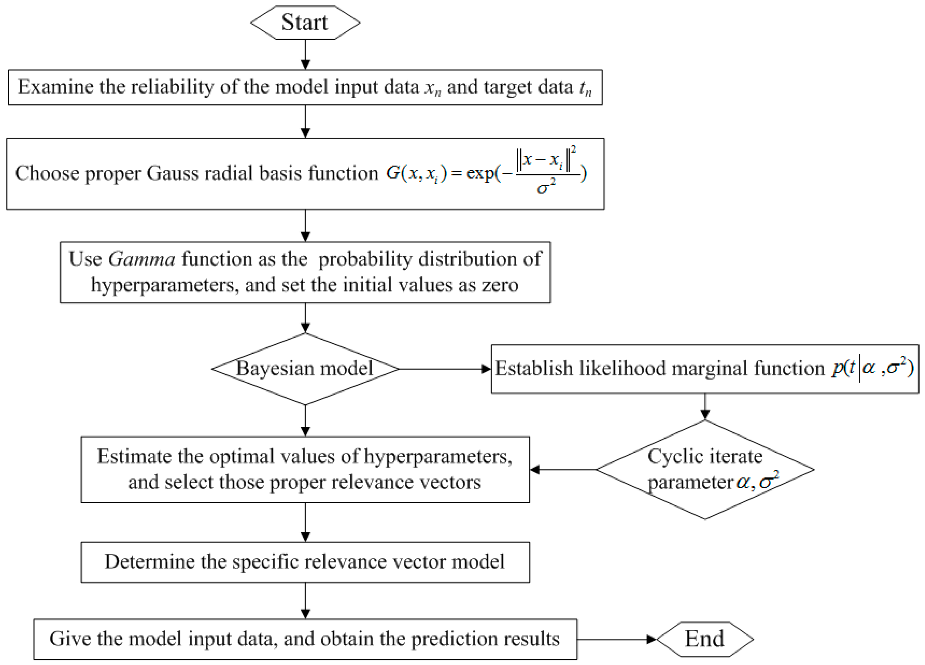
After selecting the predictor factors for the annual streamflow forecasting in the DHF and DJK Reservoir, we determine the specific RVM model through the training and testing practice using different data (

Table 4. Data used for training and testing the relevance vector machine (RVM) model and support vector machine (SVM) model in the Dahuofang (DHF) and Danjiangkou (DJK) Reservoir.

Area	Data for Model Training	Data for Model Testing
DJK	1962–2000	2001–2006
DHF	1957–2000	2001–2006

). The Gauss radial basis function (RBF) is used as the Kernel function of RVM here. Various studies have indicated the favorable performance of the RBF kernel in hydrological forecasting [17,34,35,36]. In the RVM model, the “leave-one-out” cross validation is used to optimize parameters σ, as the width of the RBF kernel. Through calculation, the optimal value 2.25 and 3.00 of parameter σ is determined for the DHF and DJK Reservoir respectively. Furthermore, we also compare the results gotten from RVM with those from SVM.

4.2. Model Performance Evaluation

Three quantitative indexes are used to evaluate the effectiveness of the RVM and SVM model, including correlation coefficient (R), root means squared error (RMSE) and Nash Sutcliffe Efficiency Coefficient (E), with the computation equations as:

$$\begin{array}{l}\mathrm{R}=\frac{\frac{1}{n}{\displaystyle \sum _{i=1}^n(Q_0(i)-\overline{Q_o})(Q_f(i)-\overline{Q_f})}}{\sqrt{\frac{1}{n}{\displaystyle \sum _{i=1}^n{(Q_0(i)-\overline{Q_o})}^2}}\sqrt{\frac{1}{n}{\displaystyle \sum _{i=1}^n{(Q_f(i)-\overline{Q_f})}^2}}}\\ \mathrm{RMSE}=\sqrt{\frac{1}{n}{\displaystyle \sum _{i=1}^n{(Q_f(i)-Q_0(i))}^2}}\\ \mathrm{E}=1-\frac{{\displaystyle \sum _{i=1}^n{(Q_0(i)-Q_f(i))}^2}}{{\displaystyle \sum _{i=1}^n{(Q_0(i)-Q_0)}^2}}\end{array}$$

(8)

where $n$ is the number of years, $Q_0(i)$ are the observed values, $\overline{Q_o}$ is the average observed values, $Q_f(i)$ are the predicted values and $\overline{Q_f}$ is the average predicted values. The R is an index used commonly to describe the correlation of two series. The RMSE can measure the difference between the observation and simulated data. The E coefficient is widely used for the evaluation of model’s performance. Generally, high NSE and R values, and small RMSE values, reflect good modeling performance [37].

4.3. Results Discussion

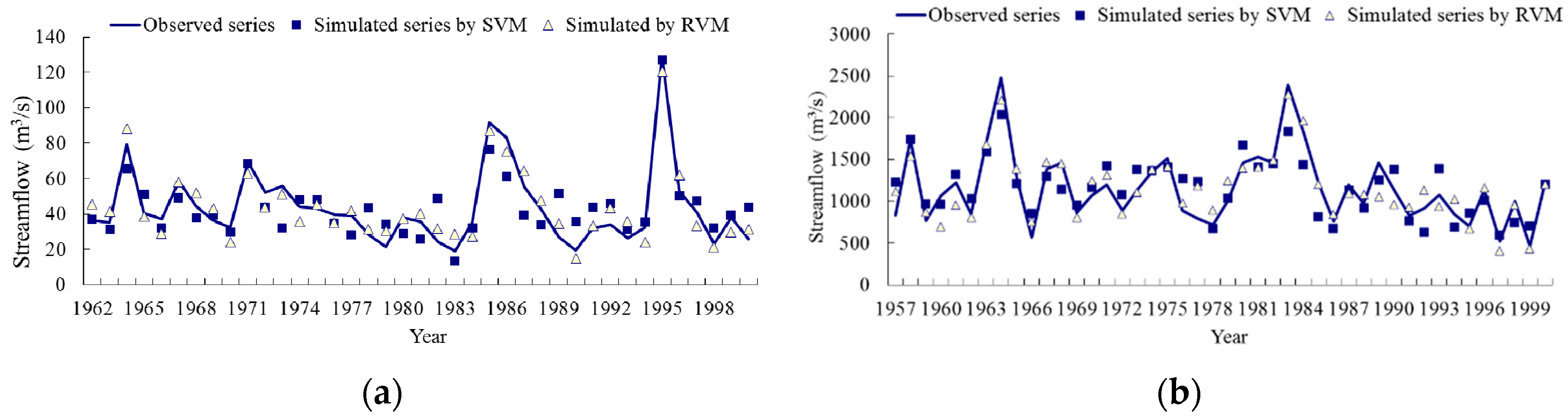
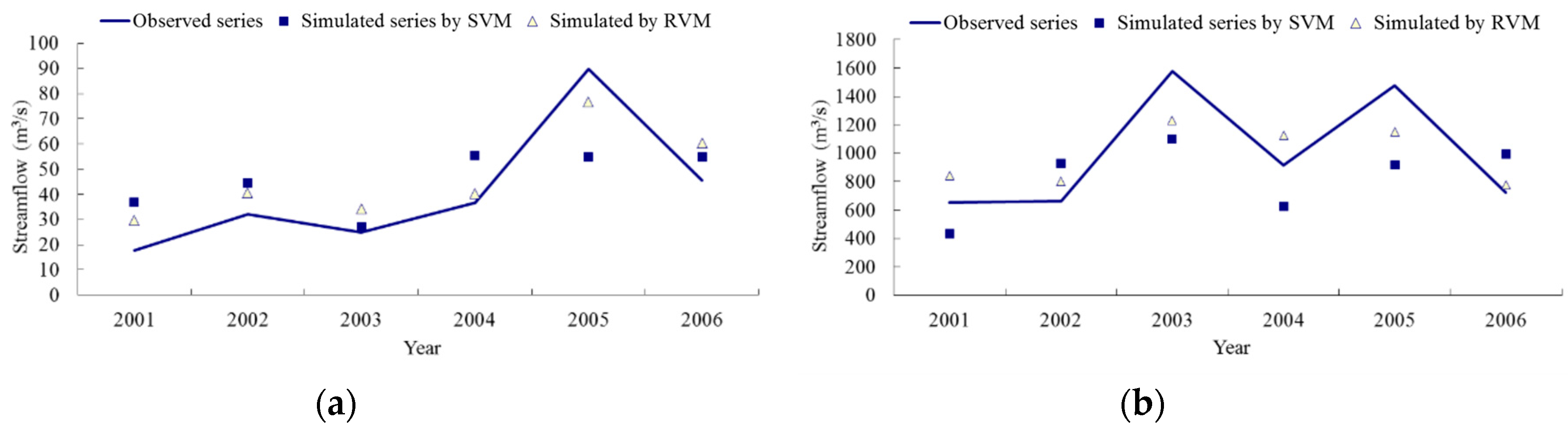
The observed streamflow data and the simulated data by SVM and RVM during the training period are shown in Figure 3 (left, DHF Reservoir; right, DJK Reservoir). The observed data and the simulated streamflow data by SVM and RVM during the testing period can be found in Figure 4 (left, DHF Reservoir; right, DJK Reservoir). In Figure 3 and Figure 4 the solid line represents the observed data, and the hollow triangle shows the simulated data gotten from the RVM model, with the solid square indicating the simulated data by SVM.

Table 5. Results of indices used to evaluate the performance of the relevance vector machine (RVM) and support vector machine (SVM) model for streamflow forecasting in the Dahuofang Reservoir.

Model	Training			Testing
	R	RMSE (m3/s)	E	R	RMSE (m3/s)	E
SVM	0.91	7.58	0.89	0.74	19.01	0.63
RVM	0.95	6.78	0.90	0.83	13.76	0.78

shows the forecasting performance of different models for the DHF Reservoir, and the results of the DJK Reservoir are presented

Table 6. Results of indices used to evaluate the performance of the relevance vector machine (RVM) and support vector machine (SVM) model for streamflow forecasting in the Danjiangkou Reservoir.

Model	Training			Testing
	R	RMSE (m3/s)	E	R	RMSE (m3/s)	E
SVM	0.84	191.18	0.81	0.67	339.01	0.57
RVM	0.92	163.06	0.85	0.88	231.92	0.68

.

From Table 5 we can find that for the streamflow forecasting in the DHF Reservoir, the values of three indices R, RMSE and E in the training period, gotten from the SVM model, are 0.91, 7.58 m³/s and 0.89, which are similar as those gotten from the RVM model, with the R, RMSE and E value of 0.95, 6.78 m³/s and 0.90. However, the RVM model performs much better than the SVM model during the testing period. To be specific, the indices R and E in the testing period gotten from the SVM model is 0.74 and 0.63, which are much smaller than those of 0.83 and 0.78 for the RVM model, but the index RMSE value of 19.01 m³/s for the SVM model is much bigger than that of 13.76 m³/s for the RVM model. The results from the DHF Reservoir indicate the better performance of the RVM model compared with SVM. Many previous studies used the traditional auto-regression models and the ANN, wavelet-based ANN models to conduct streamflow forecasting in the DHF reservoir [38,39]. Those results indicated the poor performance of the auto-regression models, which are just based on linear characteristics and long-memories of time series, and cannot deal with the decadal variability of streamflow process; besides, although those results gotten from the ANN or wavelet-based ANN models considered the influences of climate factors, they had the relative errors bigger than 20%. Comparatively, the results gotten form the RVM model in this study have higher accuracy, thus it is thought that RVM also performs better than those traditional auto-regression models and ANN models.

As for the DJK Reservoir, the results gotten from the RVM model are also much better than those of the SVM model, no matter considering the training period or testing period. In the training period, the RVM model reduces the RMSE value with respect to SVM by 14.7% (163.06 m³/s compared to 191.18 m³/s), and increase the R and E value by 9.5% (0.92 compared to 0.84) and 4.9% (0.85 compared to 0.81) respectively. In the testing period, the RVM model reduces the RMSE value by 31.6% (231.92 m³/s compared to 339.01 m³/s) compared with SVM, and increase the R and E value by 31.3% (0.88 compared to 0.67) and 19.3% (0.68 compared to 0.57) respectively. Previous studies have compared the different capabilities of the traditional auto-regression models and ANN models with that of the SVM model [40], and indicated that the forecasting results gotten from the later have high accuracy, more stability and reliability. By comprehensively analyzing the results here and the previous study results, it can be found that the RVM model performs the best among these models for the streamflow forecasting in the DJK reservoir.

Presently the SVM model has been widely applied in the streamflow simulation and forecasting, and a great number of studies have verified the ability of the SVM model in vast majority of cases; especially, its better performance compared with conventional auto-regression models or ANN models has been clearly verified in the DJK reservoir basin. Therefore, SVM can be taken as the reference to evaluate the ability of the RVM model, while other data-driven models and the results gotten from them, as discussed above, were not considered and compared again. On the whole, all the results in the two reservoirs indicate the better performance of RVM compared with SVM for long-term streamflow forecasting, although the results in the testing period is a little worse compared with those in the training period. In addition, our previous study results also indicated the better performance of the RVM model for monthly and seasonal streamflow forecasting in the two reservoirs, compared with the SVM model [41,42]. Because the RVM model is based on the Bayesian theory, posterior distributions of all parameters and characteristics of hydrological variables can be accurately and reasonably evaluated, following which more accurate forecasting results can be gotten, but the SVM model cannot do this. Thereby, it is thought that the RVM model can be effective method for long-term streamflow forecasting.

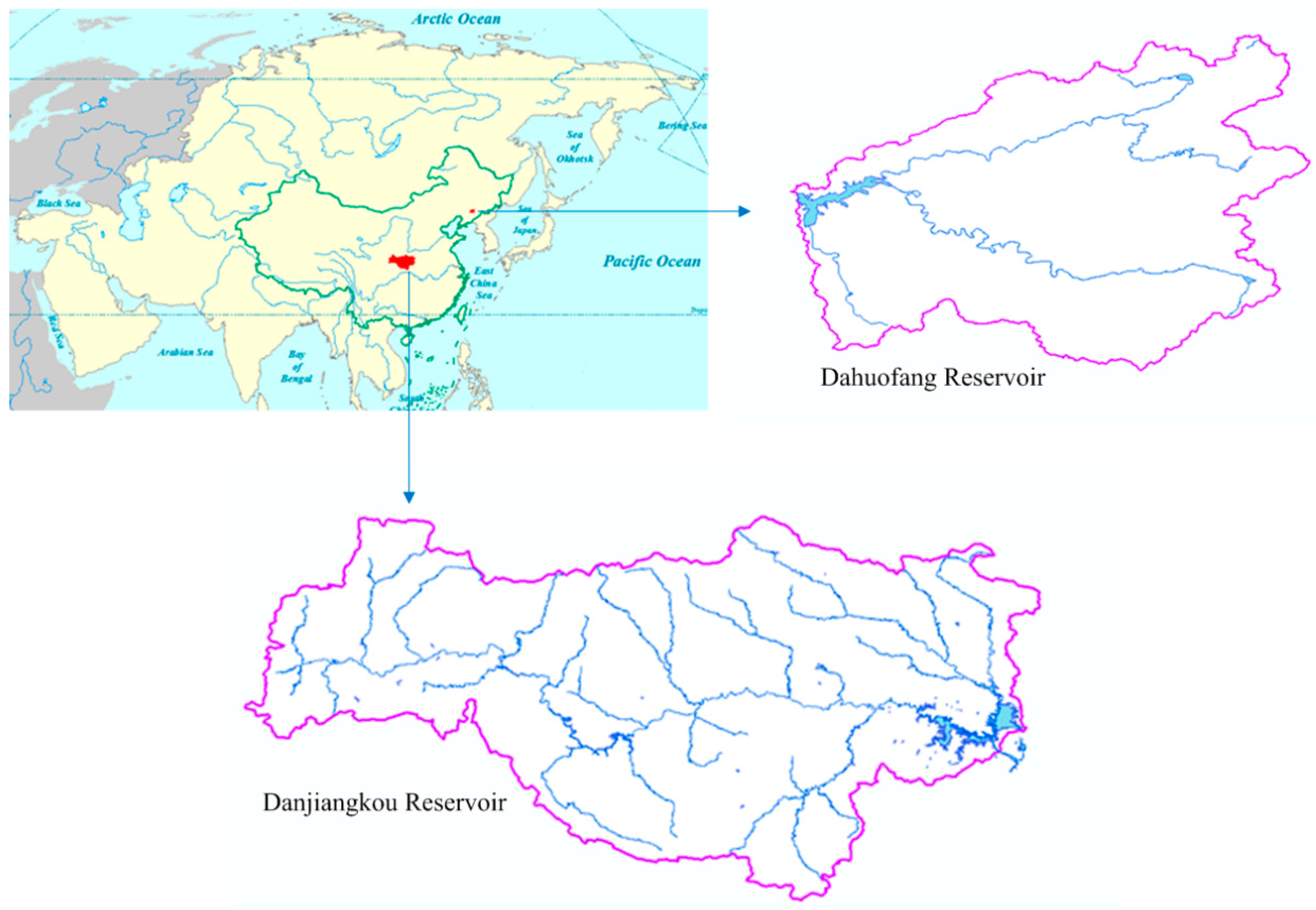
Besides, the two reservoir basins chosen for the study have obviously different underlying surface conditions and climate conditions; further, the average streamflow magnitudes in the two basins are about 40 m³/s and 1000 m³/s, also showing obvious difference. It can be found that the results in the DHF Reservoir is better that that in the DJK Reservoir when using the SVM model, indicating the worse performance of the SVM model for those streamflow process with big magnitudes. From Figure 3 we know that both the RVM and SVM model show good performance for the forecasting of peak and small values of streamflow process in the DHF Reservoir; however, peak values of streamflow process in the DJK Reservoir can only been accurately simulated by the RVM model, which cannot be achieved by the SVM model. Especially, for those peak values bigger than 2000 m³/s in the streamflow process in the DJK Reservoir, the relative errors gotten from RVM are about 20% in 2003 and 2005, but the results of SVM are much worse, with the relative errors bigger than 40%. As a result, it is thought here that the limited ability of forecasting peak magnitudes of streamflow process cause the poor performance of the SVM model. Comparatively, all the results gotten from the RVM model are stable and accurate, not matter analyzing the DHF or DJK Reservoir. Therefore, it is thought that the RVM model also has a wide applicability for long-term forecasting of streamflow process with a magnitude of dozens to thousands discharge units.

5. Conclusions

Long-term streamflow forecasting is an important issue for the reservoir scheduling and water resources management, but it is also a difficult task due to the complexity in streamflow process. In the article, we presented a data-driven model, called RVM, for annual streamflow forecasting. The RVM model was applied to the DHF Reservoir in Northern China and the DJK Reservoir in Central China. Results indicate the better performance of the RVM model compared with the SVM model which has been widely used for hydrological forecasting. Therefore, RVM can be a more reliable and effective model for long-term streamflow forecasting rather than SVM. Compared with SVM, the RVM model has relatively limited applications in the hydrology and water resources studies. Through this study, we can find the RVM model is suitable for the forecasting of annual streamflow process with obviously different magnitudes in two different basins, thus it is thought that the RVM model has a widely applicable scopes for long-term hydrological forecasting. In the future, more studies can focus on the RVM model by applying it to various basins with different climatic conditions.

References

1. Sagarika, S.; Kalra, A.; Ahmad, S. Evaluating the effect of persistence on long-term trends and analyzing step changes in streamflows of the continental United States. J. Hydrol. 2014, 517, 36–53. [Google Scholar] [CrossRef]
2. Shortridge, J.E.; Guikema, S.D.; Zaitchik, B.F. Machine learning methods for empirical streamflow simulation: A comparison of model accuracy, interpretability, and uncertainty in seasonal watersheds. Hydrol. Earth Syst. Sci. 2016, 20, 2611–2628. [Google Scholar] [CrossRef]
3. Sang, Y.F.; Singh, V.P.; Wen, J.; Liu, C.M. Gradation of complexity and predictability of hydrological processes. J. Geophys. Res. 2015, 120, 5334–5343. [Google Scholar] [CrossRef]
4. Sorooshian, S.; Dracup, J.A. Stochastic parameter estimation procedures for hydrologie rainfall-runoff models: Correlated and heteroscedastic error cases. Water Resour. Res. 1980, 16, 430–442. [Google Scholar] [CrossRef]
5. Sang, Y.F. Improved wavelet modeling framework for hydrologic time series forecasting. Water Resour. Manag. 2013, 27, 2807–2821. [Google Scholar] [CrossRef]
6. Zealand, C.M.; Burn, D.H.; Simonovic, S.P. Short term streamflow forecasting using artificial neural networks. J. Hydrol. 1999, 214, 32–48. [Google Scholar] [CrossRef]
7. Nourani, V.; Baghanam, A.H.; Adamowski, J.; Kisi, O. Applications of hybrid wavelet–artificial intelligence models in hydrology: A review. J. Hydrol. 2014, 514, 358–377. [Google Scholar] [CrossRef]
8. ASCE Task Committee. Artificial neural networks in hydrology II: Hydrologic applications. J. Hydrol. Eng. 2000, 5, 124–137. [Google Scholar]
9. Gutierrez, F.; Dracup, J.A. An analysis of the feasibility of long-range streamflow forecasting for Colombia using El Nino–Southern Oscillation indicators. J. Hydrol. 2001, 246, 181–196. [Google Scholar] [CrossRef]
10. Olsson, J.; Uvo, C.B.; Jinno, K.; Kawamura, A.; Nishiyama, K.; Koreeda, N. Neural networks for rainfall forecasting by atmospheric downscaling. J. Hydrol. Eng. 2004, 9, 1–12. [Google Scholar] [CrossRef]
11. Guven, A.; Aytek, A.; Yuce, M.I.; Aksoy, H. Genetic programming-based empirical model for daily reference evapotranspiration estimation. Clean-Soil Air Water 2008, 36, 905–912. [Google Scholar] [CrossRef]
12. Maier, H.R.; Dandy, G.C. Neural networks for the prediction and forecasting of water resources variables: A review of modeling issues and applications. Environ. Model. Softw. 2000, 15, 101–124. [Google Scholar] [CrossRef]
13. Dawson, C.W.; Wilby, R.L. Hydrological modeling using artificial neural networks. Prog. Phys. Geogr. 2001, 25, 80–108. [Google Scholar] [CrossRef]
14. Chau, K.W. Particle swarm optimization training algorithm for ANNs in stage prediction of Shing Mun River. J. Hydrol. 2006, 329, 363–367. [Google Scholar] [CrossRef]
15. Vapnik, V.N. Statistical Learning Theory; Wiley: New York, NY, USA, 1998. [Google Scholar]
16. Vapnik, V. The Nature of Statistical Learning Theory; Springer: New York, NY, USA, 1995. [Google Scholar]
17. Asefa, T.; Kemblowski, M.; McKee, M.; Khalil, A. Multi-time scale stream flow predictions: The support vector machines approach. J. Hydrol. 2006, 318, 7–16. [Google Scholar] [CrossRef]
18. Lu, M.; Zhang, Z.Y. Application of support vector machine in runoff forecast. China Rural Water Hydropower 2006, 2, 47–49. [Google Scholar]
19. Li, Y.B.; Huang, Q.; Xu, J.X.; Zuo, W.B. Research on prediction of streamflow based on C-SVM. J. Hydroel. Eng. 2008, 27, 42–47. [Google Scholar]
20. Lin, J.Y.; Cheng, C.T.; Chau, K.W. Using support vector machines for long-term discharge prediction. Hydrol. Sci. J. 2006, 51, 599–612. [Google Scholar] [CrossRef]
21. Tipping, M.E. The relevance vector machine. Adv. Neural Inf. Process. Syst. 1999, 12, 652–658. [Google Scholar]
22. Tipping, M.E. Sparse Bayesian learning and the relevance vector machine. J. Mach. Learn. Res. 2001, 1, 211–244. [Google Scholar]
23. Tripathi, S.; Govindaraju, R.S. On selection of kernel parametes in relevance vector machines for hydrologic applications. Stoch. Environ. Res. Risk Assess. 2007, 21, 747–764. [Google Scholar] [CrossRef]
24. Zaman, B.; McKee, M.; Neale, C.U. Fusion of remotely sensed data for soil moisture estimation using relevance vector and support vector machines. Int. J. Remote Sens. 2012, 33, 6516–6552. [Google Scholar] [CrossRef]
25. He, F.; Li, M.; Yang, J.H.; Xu, J.W. Product quality model based on wavelet relevance vector machine. J. Univ. Sci. Technol. Beijing 2009, 31, 934–937. [Google Scholar]
26. Hurrell, J.W. Decadal trends in the North Atlantic Oscillation: Regional temperatures and precipitation. Science 1995, 269, 676–679. [Google Scholar] [CrossRef] [PubMed]
27. Hamlet, A.F.; Lettenmaier, D.P. Columbia River streamflow forecasting based on ENSO and PDO climate signals. J. Water Resour. Plan. Manag. 1999, 125, 333–341. [Google Scholar] [CrossRef]
28. Shahab, A.; Donald, H.B.; Mohammand, K. Long-term probabilistic forecasting of streamflow using ocean-atmospheric and hydrological predictors. Water Resour. Res. 2006, 42, W03431. [Google Scholar]
29. McCabe, G.J.; Betancourt, J.L.; Hidalgo, H.G. Associations of decadal to multidecadal sea-surface temperature variability with upper Colorado River flow. J. Am. Water Resour. Assoc. 2007, 43, 183–192. [Google Scholar] [CrossRef]
30. Glenn, A.T.; Thomas, C.P.; Felipe, G. The relationships between pacific and Atlantic ocean sea surface temperatures and Colombian streamflow variability. J. Hydrol. 2008, 349, 268–276. [Google Scholar]
31. Kalra, A.; Ahmad, S. Using oceanic-atmospheric oscillation for long lead time streamflow forecasting. Water Resour. Res. 2009, 45, W03413. [Google Scholar] [CrossRef]
32. Ghosh, S.; Mujumdar, P.P. Statistical downscaling of GCM simulations to streamflow using relevance vector machine. Adv. Water Resour. 2008, 31, 132–146. [Google Scholar] [CrossRef]
33. Turing, A.M. Computing machinery and intelligence. Mind 1950, 59, 433–460. [Google Scholar] [CrossRef]
34. Khalil, A.F.; McKee, M.; Kemblowski, M.; Asefa, T.; Bastidas, L. Multiobjective analysis of chaotic dynamic systems with sparse learning machines. Adv. Water Resour. 2006, 29, 72–88. [Google Scholar] [CrossRef]
35. Gill, M.K.; Asefa, T.; Kemblowski, M.W.; McKee, M. Soil moisture prediction using support vector machines. J. Am. Water Resour. Assoc. 2006, 42, 1033–1046. [Google Scholar] [CrossRef]
36. Yu, X.; Liong, S.Y. Forecasting of hydrologic time series with ridge regression in feature space. J. Hydrol. 2007, 332, 290–302. [Google Scholar] [CrossRef]
37. Gupta, H.V.; Kling, H.; Yilmaz, K.K.; Martinez, G.F. Decomposition of the mean squared error and NSE performance criteria: Implications for improving hydrological modelling. J. Hydrol. 2009, 377, 80–91. [Google Scholar] [CrossRef]
38. You, H.L. Study on Method Application of Mid-long-term Runoff Forecast of Dahuofang Reservoir. Master’s Thesis, Liaoning Normal University, Dalian, China, 2010. [Google Scholar]
39. Dong, Y.; Yuan, J.; Zhou, H. Research on Annual Runoff Forecasting Method for Dahuofang Reservoir. J. China Hydrol. 2008, 28, 54–56, (In Chinese with English Abstract). [Google Scholar]
40. Ran, D.; Li, M.; Wu, S.; Xie, J. Research on multi-model forecasts in mid-long term runoff in Danjiangkou Reservoir. J. Hydraul. Eng. 2010, 41, 1069–1073, (In Chinese with English Abstract). [Google Scholar]
41. Hu, X.; Wang, Y.; Liu, Y.; Hu, Q. Monthly runoff forecast for Danjiangkou Reservoir based on physical statistical methods. J. Hohai Univ. Nat. Sci. 2011, 39, 242–247, (In Chinese with English Abstract). [Google Scholar]
42. Liu, Y.; Wang, Y.; Chen, Y. Long-term runoff forecasting for autumn flooding seasons in Danjiangkou reservoir based on analyzing the physical causes. Adv. Water Sci. 2010, 21, 41–48, (In Chinese with English Abstract). [Google Scholar]
Figure 1. Flow chart of the forecasting process of hydrological variables using the Relevance Vector Machine (RVM) model.
Water 09 00009 g001
Figure 2. Location of the Dahuofang Reservoir Basin and the Danjiangkou Reservoir Basin in China.
Water 09 00009 g002
Figure 3. Observed and simulated streamflow data in the Dahuofang Reservoir (a) and Danjiangkou Reservoir (b) during the training period by the RVM and SVM model.
Water 09 00009 g003
Figure 4. Observed and simulated streamflow data in the Dahuofang Reservoir (a) and Danjiangkou Reservoir (b) during the testing period by the RVM and SVM model.
Water 09 00009 g004