Calculation of Steady-State Evaporation for an Arbitrary Matric Potential at Bare Ground Surface


Department of Geology and Geophysics, Texas A&M University, College Station, TX 77843-3115, USA
*
Author to whom correspondence should be addressed.
Water 2017, 9(10), 729; https://doi.org/10.3390/w9100729
Submission received: 10 July 2017
/
Revised: 13 September 2017
/
Accepted: 19 September 2017
/
Published: 22 September 2017
(This article belongs to the Special Issue Advances in Groundwater Flow and Solute Transport: Pushing the Hidden Boundary)
Abstract
:Evaporation from soil columns in the presence of a water table is a long lasting subject that has received great attention for many decades. Available analytical studies on the subject often involve an assumption that the potential evaporation rate is much less than the saturated hydraulic conductivity of the soil. In this study, we develop a new semi-analytical method to estimate the evaporation rate for an arbitrary matric potential head at bare soil surface without assuming that the potential evaporation rate is much less than the saturated hydraulic conductivity of the soil. The results show that the evaporation rates calculated by the new solutions fit well with the HYDRUS-1D simulation. The new solutions also can reproduce the results of potential evaporation rate calculated from previous equations under the special condition of an infinite matric potential head at bare soil surface. The developed new solutions expand our present knowledge of evaporation estimation at bare ground surface to more general field conditions.
1. Introduction
Evapotranspiration is one of the most important components in the study of the hydrological cycle, as it controls the exchange of mass and energy among the soil–water–vegetation system, the atmosphere and the groundwater system. Understanding water loss from soil by evapotranspiration due to the upward water flow from a water table is an important topic in many disciplines such as soil sciences [1], hydrology [2], and plant physiology [3]. The evapotranspiration comprises three processes: evapotranspiration from vegetated surfaces, evaporation from bare ground surfaces, and evaporation from open water bodies. The water exchange among soil, vegetation and atmosphere determines to a large extent the regional climate and the behavior of the hydrological cycle [4]. Land use is considered a local environmental issue and has a great influence on the hydrological circle [5,6], especially on the evapotranspiration as it alters the upper soil layer and land cover. Land cover features are part of the hydrological system, and the changes of land cover can impact evapotranspiration with the increasing expansion of urban areas, which causes permeable land reduction and increased flooding [5]. Furthermore, some previous studies show that vegetation and agriculture tend to increase evapotranspiration, and urbanization tends to decrease evaporation [7,8]. These effects of land use change on evapotranspiration need to be considered in water management study. The accurate estimation of evaporation from bare ground surface is important in determining the overall processes of evapotranspiration and will be the primary focus of this study. Direct measurement of soil evaporation is difficult and the most commonly used method involves a weighing lysimeter [9]. Although water evaporation in actual field setting is a highly complex process, a nearly steady upward flow from a water table to a bare soil surface may be established if the daily evaporative demand is reasonably uniform for a long period of time [10]. Water content in soil controls vertical water flow direction and velocity, and soil property affects water holding capacity and water flow velocity as well. While the soil moisture and matric potential head at the ground surface depend on atmospheric and soil conditions, the actual flux through the soil surface should be limited by the ability of the porous medium to transmit water from the unsaturated zone.
In terms of evaporation calculation, two scenarios are commonly seen. The first scenario deals with an evaporative front that is located at the ground surface. This is usually true when the water table is relatively shallow and the upward capillary liquid flow is sufficient to maintain a hydraulic connection between the water table and the ground surface. The second scenario deals with an evaporative front that is below the ground surface. For such a scenario, the upward capillary flow may not be strong enough to overcome the downward gravity, resulting in discontinuity of the vertical liquid profile at a certain level below the soil surface [11]. In other words, a water-depletion dry layer will be formed between the ground surface and the evaporative front, which marks the discontinuity of the liquid profile. In this case, the evaporative process is composed of an upward capillary liquid flow from the water table to the evaporative front (or vaporization plane) and a vapour diffusion through the upper dry layer. Many studies have been devoted to this subject, such as Rose et al. [12], Gowing et al. [13], Il’ichev et al. [14], Lehmann et al. [15], Shokri et al. [16], and Shokri and Salvucci [11].
The results from Gowing et al. [13] showed that the vaporization plane usually resided 4–14 cm below the ground surface for saline or non-saline soils. Assouline et al. [17] pointed out that the thickness of the dry layer above the vaporization plane varied within a relatively narrow range from 3 to 20 mm. Some studies have specifically discussed the maximum depth of the water table hydraulically connected to the ground surface via continuous capillary liquid pathways [11,18,19]. When the water table is deeper than the maximum depth hydraulically connected to the surface, the capillary flow will be disrupted. Lehmann et al. [20] and Sadeghi et al. [21] discussed a method to estimate the maximum matric potential at the bare ground surface that would maintain the hydraulic connections of the vertical unsaturated profile above the water table. Hayek [22] presented an analytical model for the steady-state vertical flow condition that could estimate the length of liquid phase and gas phase in the unsaturated zone.
Several researchers developed steady-state water flow solutions through a soil profile from a water table to bare ground surface (e.g., [12,13,23,24,25]). For instance, Gardner [23] developed a steady-state solution to show the relationship among the maximum evaporation rate, the capillary conductivity and the water table depth. Warrick [25] modified the form of unsaturated conductivity function as that of Brooks and Corey [26] and developed an exact solution for the maximum evaporation rate. Salvucci [24] developed approximate evaporation rate solutions on the basis of the Gardner and the Brooks–Corey functions, and such approximate solutions agreed considerably well with experimental results of three types of soils, as reported in Bras [27]. Rose et al. [12] and Gowing et al. [13] studied the evaporation flow from saline groundwater considering the salt accumulation effect. Gowing et al. [13] developed a solution when both liquid-phase and vapour-phase flows were of concern.
This study will address the first scenario with the evaporative front at the ground surface. The second scenario (with an evaporative front below the ground surface) will be addressed in a future investigation. In semi-arid or arid regions where surface vegetation is sparse or sometimes non-existent, water loss from the bare ground surface may be a grave concern in terms of water management and ecological conservation, among many other aspects. Precise determination of evaporation from bare ground surface in semi-arid or arid regions then becomes critically important, which will be the focus of this article.
The purpose of this article is to develop a new semi-analytical approach for calculating evaporation from a bare surface with an arbitrary matric potential at the surface. These newly developed solutions are more general than previously available solutions, which often involve an assumption that the matric potential at the surface is infinitely large, an assumption that is questionable in actual field applications. This study only considers the liquid flow phase of the evaporative process and does not consider the vapor flow phase, which is often much smaller than the liquid flow, as shown in many previous studies [12,15]. As bare ground is of concern here, plant transpiration is also excluded.
The paper is organized as follows. A mathematical model is built and solutions are developed in Section 2, followed by analysis of results in Section 3, including testing the new solutions against previous benchmark solutions under various special conditions, and comparing the new solutions with numerical simulations using HYDRUS-1D. Section 4 and Section 5 discuss the results of comparison among new solutions, HYDRUS-1D and previous works, and summarize the major conclusions of this study.
2. Mathematical Model
2.1. Background and Problem Description
In many previous studies of the steady-state evaporation from bare surface, Gardner’s unsaturated hydraulic conductivity model [23] has been used widely. When the unsaturated hydraulic conductivity–depth relationship is known, the steady-state upward water flow across the soil profile follows the Buckingham–Darcy flow law [28] as
where the z-axis is positive upward with z = 0 at ground surface, h is the matric potential head (negative) [L], K(h) is the unsaturated hydraulic conductivity [LT−1], and E is the upward water flux [LT−1], which is equal to the value of evaporation rate at bare ground surface under the steady-state flow condition. A fixed water table is assumed to be below the ground surface at a distance L (z = −L). Only the vertical flow is of concern here, and the lateral flow is assumed to be secondary and negligible. The soil profile is assumed to be vertically homogeneous, thus soil layering and heterogeneity is not considered at this study. However, soil heterogeneity is an important feature and may be considered in a future investigation on the basis of this study.
Gardner [23] developed two widely used unsaturated hydraulic conductivity models. The first one was:
where Ks is the saturated hydraulic conductivity [LT−1] and is a fitting parameter related to the pore size distribution of soil [L−1]. The second one was
where A, B, and N are positive empirical factors related to soil texture and is a sign of absolute value [29].
Equation (1) shows that the evaporation rate often depends on the depth to the water table, the matric potential at the soil surface, and the hydraulic conductivity of soil. Gardner [23] revealed that when the matric potential at the surface was infinity, the evaporative flux would approach a maximum rate that was a function of the saturated hydraulic conductivity, the fitting parameters N, A, B in Equation (1) and the depth to the water table.
Haverkamp et al. [30] amended the parameters of Equation (3) and made the equation more concise, which is denoted as the modified Gardner model hereinafter. Jury and Horton [10] proposed a method of calculating the potential evaporation rate above a water table on the basis of the modified Gardner model [30] and an assumption that the potential evaporation rate was much less than the saturated hydraulic conductivity. Such an assumption was debatable in many field conditions. For instance, when the water table is reasonably shallow, the potential evaporation rate should increase to a value that is close to or even larger than the value of the saturated hydraulic conductivity. Nevertheless, Jury and Horton [10] presented a one-dimensional model to describe water flow from a shallow water table upward to an evaporating surface using such an assumption.
The modified Gardner model by Haverkamp et al. [30] involves an unsaturated soil hydraulic conductivity as a function of the matric potential head h [L] (negative) as follows:
where a is a characteristic length [L] (negative). It is worthwhile to point out that Equation (4) is a special case of Equation (3) by setting B = A and A = in Equation (3). Equation (4) is called the modified Gardner model hereinafter.
When steady-state flow is of concern, applying the Buckingham–Darcy law to vertical flow, one has:
Reorganizing Equation (5) into an integral, one has:
where h1 = h(z1) and h2 = h(z2) are two matric potential heads at two different elevations z1 and z2, respectively. In the problem studied below, we set z1 = −L (water table) and h1(−L) = 0; z2 = 0 (ground surface) and h2(0) = h0, which is a constant matric potential head at ground surface. Substituting Equation (4) into Equation (6) leads to
Defining a new parameter µ = h/a and µ0 = h0/a, which are positive, and substituting them into Equation (7) one has:
Be aware that –L/a on the right side of Equation (8) is positive because a is a negative constant.
Defining the following new parameters: , and , one transforms Equation (8) into:
For the special case of calculating the potential evaporation rate, one may apply the negatively infinite matric potential head at ground surface or a positively infinite σ0 in Equation (9). Under this condition, one can employ the following identity [31]:
Substituting Equation (10) into Equation (9) for the case of and recalling the definition of will lead to the following equation:
where Ep in Equation (11) represents the potential evaporation rate hereinafter.
Equation (11) can be used to calculate the potential evaporation rate. The form of Equation (11) does not permit a direct analytical estimation of Ep for a general soil type, and one has to seek help from a numerical root-searching method. Under the special condition that Ep/Ks is much less than 1, one can obtain a closed-form solution for Ep based on Equation (11):
The purpose of Equation (12) is to simplify the calculation process of Equation (11) so that one can obtain a closed-form analytical solution for Ep, as reported by Jury and Horton [10]. However, as the assumption that Ep/Ks is much less than 1 may not hold in actual field conditions, one must be cautious for using Equation (12) for estimating Ep for cases where Ep/Ks is not much less than 1. One question is that of how much error may be introduced for using Equation (12) for a certain Ep/Ks value that is not too much less than 1. To answer this question, one needs to develop an accurate solution for a more general case that Ep/Ks is permitted to vary over a wide range of allowable values, which is developed in the following section.
2.2. New Solutions of Evaporation with Arbitrary Surface Matric Potentials
We now extend the steady-state evaporation solution to a general case with an arbitrary matric potential at the bare ground surface without using the assumption that Ep/Ks is much less than 1. Our solutions are based on two popular unsaturated hydraulic conductivity models: the modified Gardner [23] model and the Brooks–Corey [26] model in describing the unsaturated zone flow processes.
2.2.1. Calculation of Evaporation Rate E with the Modified Gardner [23] Model
When the modified Gardner [23] model is of concern (see Equation (4)), for an arbitrary matric potential head at the ground surface, σ0 is positively finite rather than infinite (as in Section 2.1) and it is given as . The integration in Equation (9) can be separated into two components: one for and one for .
If , Equation (9) can be written as:
If , one can similarly obtain:
Therefore, one can calculate the evaporation rate E on the basis of Equation (13) or Equation (14) with a given water table depth L, and parameters N, Ks, and a known from the Gardner [23] model. As E is embedded in the definition of σ0, such a calculation cannot be carried out using a closed-form solution except for the special case that is much less than 1. Rather, a numerical root-searching method such as the Newton–Raphson algorithm [32] may be used.
There are two technical issues that must be taken care of for the computation. The first issue is that since one is unclear if σ0 is greater or less than 1 before the determination of E, thus one is also unsure whether to use Equation (13) or Equation (14) to perform the computation. To address this issue, we recommend the following steps. Firstly, one should compute E from Equation (13) using the Newton–Raphson method for root-searching [32]. Secondly, after obtaining E, one will check the σ0 value with the obtained E value. If the σ0 value is indeed greater than or equal to 1, then Equation (13) is valid. If the σ0 value is less than 1, then Equation (13) is invalid and one has to use Equation (14) to calculate E.
The second issue is that one has to approximate the infinite series of summation in Equation (13) or Equation (14) by a finite series of summation with sufficient accuracy. By doing so, one can first compute E with a finite M terms approximation of Equation (13) or Equation (14), denoted as EM. After that, one will repeat the computation of E with (M + 1) terms approximation of Equation (13) or Equation (14), denoted as EM+1. Then, one can check the difference of EM and EM+1. If is less than a pre-determined small criterion such as 10−6, one can say that the infinite series of summation can be approximated with the finite M terms series of summation with sufficient accuracy. Our numerical exercises show that the M value is usually around 10–50.
2.2.2. Calculation of Evaporation Rate E with the Brooks–Corey [26] Model
The Brooks–Corey function is also widely used for water flow in unsaturated zone. It is commonly associated with Burdine’s pore size distribution model [28], leading to the hydraulic conductivity function as follows:
where p (positive) is a soil specific parameter that accounts for the tortuosity of the flow [dimensionless], λ (positive) is the pore size distribution index [dimensionless], S is the degree of saturation [dimensionless] and hv (negative) [L] is the air-entry value of h (negative). The p-value was assumed to be 1.0 in the original study of Brooks and Corey [26].
Defining the following new parameters: w = pλ + 2λ + 2, , and , where . As demonstrated in Appendix A, three equations can be obtained from Equation (6):
When , one has:
When , one has:
When , one has:
The evaporation rate E can be determined from Equations (18)–(20), following the same procedures explained in above Section 2.2.1 for the modified Gardner model, and will not repeat here.
3. Results
3.1. Check of Applicability of Equations (11) and (12)
In the past decades, several researchers [10,24,25] have studied the effect of water table depth on evaporation from ground surface. Salvucci [24] showed that when the fitting parameter N (see Equation (4)) increased, the magnitude of relative evaporation rate should decrease. Warrick [25] presented the values of the relative evaporation (E/Ks) based on the work of Gardner [23] and Brooks–Corey [26], and Warrick [25] reduced the parameter B in the Brooks–Corey model (Equation (3)) to 0 in order to make the problem analytically amendable, thus it can be regarded as a special case of the Brooks–Corey model that may not be applicable to soils with B value not equaling to or very close to zero.
Jury and Horton [10] gave two equations for calculating the bare ground evaporation, which are Equations (11) and (12) of this study. However, applicability of these two equations for actual soils is not investigated in sufficient detail. Based on four different soil types listed in Table 1, the results of calculated relative potential evaporation rates (Ep/Ks) for water table depths ranging from 10 cm to 1000 cm by Equation (11) are listed in Table 2. A few interesting observations can be made from Table 2. Firstly, when the water table is as shallow as 10 cm, Ep/Ks values for all four soil types are greater than 1.0, thus Equation (12) cannot be used to calculate the evaporation rate as this equation requires that Ep/Ks is much less than 1. Secondly, for a water table depth of 50 cm, Equation (12) is still not applicable as Ep/Ks values are not much less than 1, particularly for the case of Pachappa fine sandy loam, which has an Ep/Ks value of 0.96. Thirdly, for a water table depth of 100 cm, Equation (12) should be applicable for Buckeye fine sand and Yolo Light Clay, but is not recommended for Chino Clay and Pachappa fine sandy loam. Fourthly, for water table depth greater than 300 cm, Equation (12) is applicable for all four soil types as the Ep/Ks values are all less than 0.016.
From the above analysis, one can see that whether Ep/Ks is much less than 1 or greater than 1 depends on the soil properties and the water table depth. For instance, when the water table depth is greater than 300 cm, the Ep/Ks values for the four soil types of Table 2 are all much less than 1. However, for the same soil types, the Ep/Ks values become greater than 1 when the water table depth is as shallow as 10 cm.
To estimate the discrepancy of values produced by Equations (11) (without the assumption that Ep/Ks being much less than 1) and (12) (with the assumption that Ep/Ks being much less than 1), one may use the following formula: , where E11 and E12 represent Ep calculated from Equations (11) and (12), respectively. The results of discrepancy for five different soil types are listed in Table 3. Previous experimental data suggested the N values to be 2, 3, 4, 4, 5, and the a values to be −20.8 cm, −86.7 cm, −17 cm, −10.9 cm and −44.7 cm, respectively, for clay loam, silty loam, sandy loam, coarse sand and fine sand in Table 3, where the hydraulic properties of soils were measured by Ashraf [35,36], Rijtema [37] and van Hylckama [34].
Figure 1 [38] shows the values of Ep/Ks for a range of N and −a/L values based on Equation (11). In Figure 1, six different contours of Ep/Ks ranging from 0.05 to 0.00001 are plotted. This figure may be used to quickly estimate the range of evaporation rate based on the soil type parameters a and N for a given water table depth L. By knowing the range of Ep/Ks, one can subsequently estimate the discrepancy range of the results obtained from Equations (11) and (12) (see Table 3). Such a discrepancy range will allow us to decide if Equation (12) or Equation (11) should be used. In this study, we choose 5% discrepancy as the threshold, meaning that if the discrepancy is greater than 5%, Equation (12) is not recommended and one has to use Equation (11); if the discrepancy is less than 5%, one can use Equation (12) as a good approximation of Equation (11). For instance, when Ep/Ks are 0.05 and 0.01, the discrepancy ratios between Equations (11) and (12) for Buckeye soil (fine sand) are 17.8% and 3.9%, respectively. Then, one can conclude that Equation (12) may be applicable when Ep/Ks is 0.01, but not applicable when Ep/Ks is 0.05. However, for clay loam soil, when Ep/Ks are 0.005 and 0.01, the discrepancy ratios between Equations (11) and (12) are 4.8% and 1.0%, respectively. Therefore, Equation (12) may be applicable for both Ep/Ks of 0.005 and 0.01.
The discrepancy of 5% is a matter of authors’ choice. If necessary, a different criterion may be used. However, it is better to use a criterion of no more than 10% because of the following consideration. It is notable that the discrepancy discussed here is only theoretical. This means that additional discrepancy associated with the simplification of actual field condition into the conceptual model of this study is unknown and not considered. Therefore, if the theoretical discrepancy criterion is too large, for instance, 10%, the actual discrepancy of applying such a model for field problems would be greater than 10%, which will make the proposed solution less accurate and less reliable.
Now, one may answer the question of what range of Ep/Ks values can be regarded as much less than 1, which is an assumption used in the approximation of Equation (12) [10]. The answer depends on the accuracy requirement. For instance, if one can tolerate 5% of approximation error for the final estimation of the evaporation rate, Ep/Ks values less than 0.01 are acceptable.
3.2. Results with Brooks–Corey and Modified Gardner Models
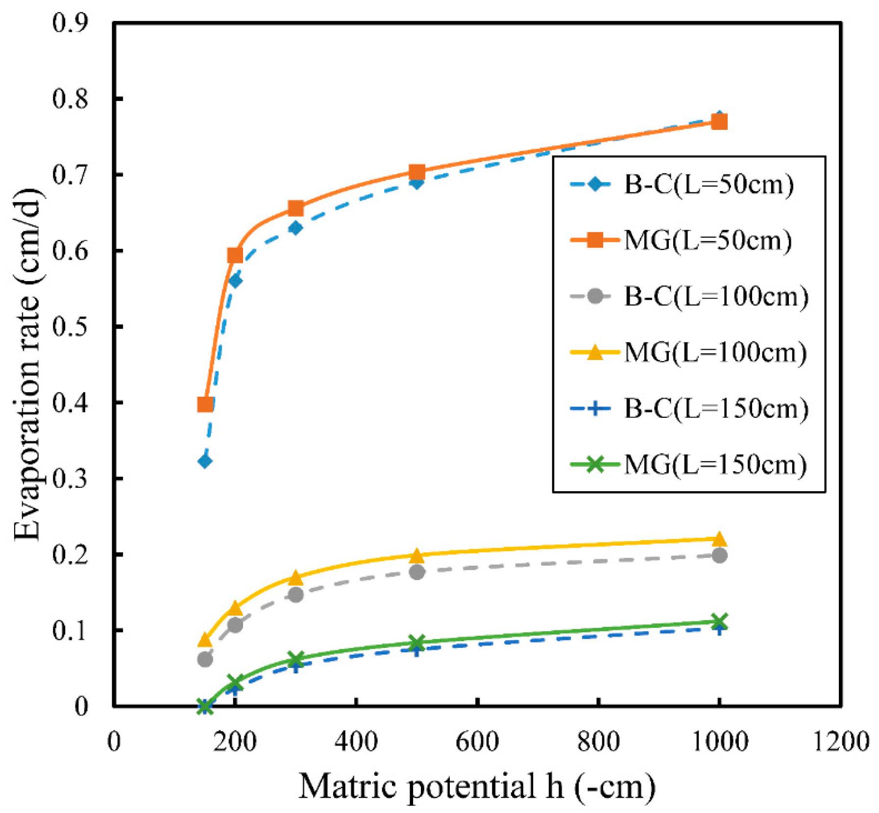
Sadeghi et al. [18] suggested that the Brooks–Corey soil parameters hv equaled the Gardner fitting parameters a, and pλ + 2λ + 2 equaled the Gardner fitting parameter N for Chino Clay. The results of evaporation rate calculated by the modified Gardner model and the Brooks–Corey model are shown in Figure 2.
The ratios of the E values calculated by the Brooks–Corey and the modified Gardner models for a water table depth of 50 cm and the surface matric potential heads of −100 cm, −200 cm, −300 cm, −500 cm and −1000 cm are 81%, 94%, 96%, 98% and 100%, respectively. The reason to include −1000 cm of surface matric potential head is to simulate the potential evaporation rate (Ep). If changing the water table depth to 100 cm, the ratios of the E values calculated by the Brooks–Corey and the modified Gardner models are 82%, 88%, 89% and 91% for the matric potential heads of −200 cm, −300 cm, −500 cm and −1000 cm, respectively. If further changing the water table depth to 150 cm, the ratios of the E values calculated by the Brooks–Corey versus the modified Gardner models are 72%, 85%, 89%, 92% for the matric potential heads of −200 cm, −300 cm, −500 cm, −1000 cm, respectively.
A few observations can be made for the comparison of the Brooks–Corey versus the modified Gardner models. First, the calculated E values from both models are not too far apart, even for the relatively small matric potential head at the surface. The smallest ratio of the E values between the Brooks–Corey model and the modified Gardner model is 72% for the water table depth of 150 cm and a matric potential head of –200 cm. Second, such a ratio increases with the magnitude of the surface matric potential head for a given water table depth. Third, the Ep values (corresponding to the −1000 cm surface matric potential head) calculated from these two models are very close to each other. For instance, for the shallower water table depth of 50 cm, the Ep values calculated from both models are essentially the same. The greatest discrepancy of the Ep ratio for the water table depth of 150 cm is only 8%.
The Brooks–Corey parameters used above are closely related to the modified Gardner parameters. However, this is not always applicable for some soil types. Rawls et al. [39] summarized the Brooks–Corey fitting parameters for eleven types of soils. Among them, we selected four representative types with the details listed in Table 4. Substituting the Brooks–Corey parameters of Table 4 into Equations (18)–(20), we calculated the evaporation rates for four types of soils under different matric potential heads at ground surface and compared the results with the simulation results of the HYDRUS-1D program. The results for the water table depths of 100 cm were shown in Figure 3. Such calculated E values are very close to their simulated counterparts by HYDRUS-1D for all the cases.
3.3. Comparison with Previous Work of Sadeghi et al. [18]
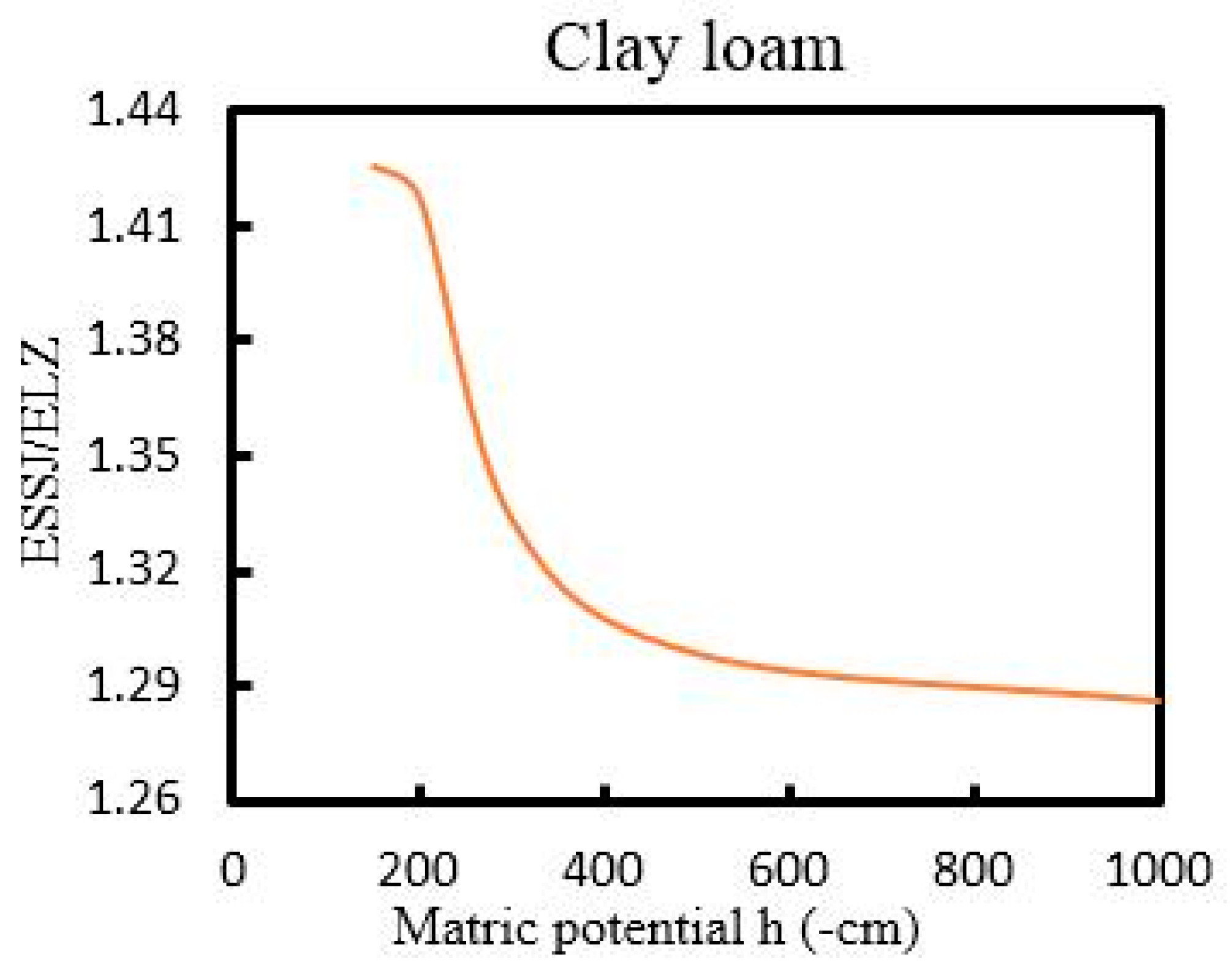
Sadeghi et al. [18] developed a closed-form solution to calculate the steady-state evaporation rate by the Brooks–Corey function. The closed-form solution is based on an assumption of “2 + (2 + p)λ is much larger than 1”. From the soil water properties estimated by Rawls et al. [39], the values of 2 + (2 + p)λ are actually not much larger than 1. From the soil properties used in Sadeghi et al. [18], there are a few soils that have large values of “2 + (2 + p)λ”. Figure 4 compares results calculated by the solution of Sadeghi et al. [18] and our solutions of Equations (18)–(20) for clay loam for a water table depth of 100 cm, where ESSJ is the evaporation rate calculated by the solution of Sadeghi et al. [18], and ELZ is our solutions of Equations (18)–(20). The values of “2 + (2 + p)λ” for four soils in Table 4 are all between 2 and 3. Figure 4 shows that the results of this study are smaller than their counterparts computed from the closed-form solution of Sadeghi et al. [18], with the ratio of ESSJ/ELZ varying between 1.43 and 1.28 for the surface matric potential head changing from −150 cm to −1000 cm. This implies that the closed-form solution of Sadeghi et al. [18] may not be accurate enough to calculate the evaporation rates in these soils.
4. Discussion
In this study, the modified Gardner model, the Brooks–Corey model and HYDRUS-1D have been used to calculate the steady-state evaporation rate for an arbitrary matric potential head at ground surface with the presence of a water table. This study is different from most previous analytical and semi-analytical studies that usually focused on estimating the potential evaporation rate at ground surface (with infinitely large matric suction at ground surface). In actual field conditions, the surface suction may be affected by the humid climate, invalidating the infinity matric suction assumption, or the actual evaporation rate may be much less than the potential evaporation rate. This study fills a gap for providing a semi-analytical method to calculate the evaporation rate under an arbitrary surface suction. The new solutions established here may also be used to estimate the difference of the potential and actual evaporation rates for a variety of conditions.
This study selects one type of soil (Chino Clay in Table 1) to demonstrate the application of the proposed method for the modified Gardner model and the Brooks–Corey model. For this soil, the fitting parameters of a and N in the modified Gardner model are directly related to the fitting parameters of p, λ, hv of the Brooks–Corey model in a fashion of N = pλ + 2λ + 2 and hv = a [18], the E values obtained from these two models fit reasonably well with some small but consistent discrepancies (Figure 2). Such small discrepancies probably come from different functions employed for describing these two models.
The comparison between the Brooks–Corey model and the HYDRUS-1D simulation is very good for all the cases. The results show that the method developed in this study is useful for general evaporation rate estimation. We also compare the solution with the analytical solution of Sadeghi et al. [18] (see Equation (11) in Sadeghi et al. [18]), and the result is less satisfactory. This is probably because the assumption that “2 + (2 + p)λ is much larger than 1” as used in Sadeghi et al. [18] is not satisfied for the type of soils used in this study (see Table 4) [39]. This statement is confirmed after a careful inspection of Sadeghi et al. [18], which also discussed the sensitivity of the p-value (which is essentially the same term as “2 + (2 + p)λ” in this paper) for their solution. In Equation (11) of Sadeghi et al. [18], if one sets z on the left side of the equation as the water table depth, one can calculate the r term that is included inside the logarithmic functions on the right side of the equation, where r is the ratio of the evaporation rate over the saturated hydraulic conductivity of the soil. However, Equation (11) of Sadeghi et al. [18] was obtained with the assumption that the p-values were much larger than 1. Therefore, it is not surprising to see that the comparison of this study and Equation (11) of Sadeghi et al. [18] is less satisfactory because the p-values for the type of soils used in this study are not much larger than 1, violating the assumption required for using Equation (11) of Sadeghi et al. [18].
It is worthwhile to carry out well-controlled experiments in the laboratory and/or the field to directly measure the evaporation rate and to compare the experimental results with the theoretical results of this study for a variety of soil types. Such experimental works are not included in this study but should be pursued in the future.
In this study, all solutions are derived under steady-state flow condition, the assumption that the temperature at the soil profile is constant, and the vadose zone being homogeneous. This study does not consider the vapor phase diffusive flow.
Since the semi-analytical approach of this study is based on very few soil samples, its applicability to a broad range of soil samples is still unclear and should be checked in the future. Furthermore, caution should be taken to apply the solutions to deal with realistic field problems, which could be much more complex than the conceptual model of this study. For instance, soil heterogeneity, including multiple layered soil profiles that exist in some actual applications, has not been considered in this study. Preferential flow, which has been seen in some soils, has also not been taken into consideration. The influence of such complex field conditions on evaporation deserves further investigation in the future.
5. Conclusions
The following conclusions can be drawn from this study:
A new mathematical model and associated solutions have been established for computing the evaporation rate at a bare ground surface with an arbitrary surface matric potential for the modified Gardner [23] model and the Brooks–Corey [26] model. The new solutions have been tested extensively against previous solutions (under special conditions) and numerical solutions obtained with HYDRUS-1D and are shown to be robust and accurate.
The comparison of the new solutions and the previous solution of Jury and Horton [10] for computing the potential evaporation rate (see Equations (11) and (12) of this study) indicates that the often used assumption of the relative potential evaporation rate (which is the ratio of potential evaporation rate over the saturated hydraulic conductivity of the soil) being much less than 1 is not established in some conditions, and the actual evaporation rate could deviate considerably from what is calculated on the basis of such an assumption.
The results of this study are smaller than their counterparts computed from the closed-form solution of Sadeghi et al. [18] with the ratio of ESSJ/ELZ varying between 1.43 to 1.28 for the surface matric potential head changing from −150 cm to −1000 cm, where ESSJ and ELZ denote the solution of Sadeghi et al. [18] and the solution of this study, respectively. This implies that the closed-form solution of Sadeghi et al. [18] may not be accurate enough to calculate the evaporation rates in some soils.
The mathematical model of this study provides a new and straightforward analytical approach to estimate evaporation rate based on a few soil parameters and matric potential on the bare ground surface. This approach is easier to use than the numerical solutions such as HYDRUS-1D, which requires a great number of input parameters and a proper discretization of the domain of interest. The solution developed in this study can also be used as a benchmark to test the numerical solutions that may suffer from various numerical errors. The limitation of the analytical approach is that it cannot deal with complex field conditions such as soil heterogeneity, preferential flow, flow transiency, and irregular boundary conditions, which may be handled by proper numerical models.
Acknowledgments
We sincerely thank four anonymous reviewers for their constructive comments which help us improve the quality of the manuscript.
Author Contributions
Hongbin Zhan and Xin Liu designed the research; Xin Liu performed the research; Hongbin Zhan and Xin Liu discussed the results and wrote the manuscript.
Conflicts of Interest
The authors declare no conflict of interest associated with this manuscript.
Appendix A
Derivation of Equations (18)–(20)
Instead of using the modified Gardner equation, one can use the Brooks and Corey [26] function in Equation (6) to get:
where E is the evaporation rate. Defining the following new parameters: w = pλ + 2λ + 2, substituting Equations (16) and (17) into Equation (A1) leads to:
Equation (A2) can be simplified as follows:
Defining the following new parameters: w = pλ + 2λ + 2, , and , where , Equation (A3) then becomes:
The integration on the left side of Equation (A4) can be dealt with using the same procedures employed in Section 2.2.1 for the modified Gardner model.
When , one has:
When , one has:
When , one has:
References
- Chanzy, A.; Bruckler, L. Significance of soil surface moisture with respect to daily bare soil evaporation. Water Resour. Res. 1993, 29, 1113–1125. [Google Scholar] [CrossRef]
- Morton, F.I. Operational estimates of areal evapotranspiration and their significance to the science and practice of hydrology. J. Hydrol. 1983, 66, 1–76. [Google Scholar] [CrossRef]
- Asbjornsen, H.; Goldsmith, G.R.; Alvarado-Barrientos, M.S.; Rebel, K.; Van Osch, F.P.; Rietkerk, M.; Chen, J.; Gotsch, S.; Tobon, C.; Geissert, D.R.; et al. Ecohydrological advances and applications in plant–water relations research: A review. J. Plant Ecol. 2011, 4, 3–22. [Google Scholar] [CrossRef]
- Feddes, R.A.; de Rooij, G.H.; van Dam, J.C. Unsaturated-Zone Modeling: Progress, Challenges and Applications; Kluwer Academic Publishers: Dordrecht, The Netherlands, 2004; 364p. [Google Scholar]
- Apollonio, C.; Balacco, G.; Novelli, A.; Tarantino, E.; Piccinni, A.F. Land Use Change Impact on Flooding Areas: The Case Study of Cervaro Basin (Italy). Sustainability 2016, 8, 996. [Google Scholar] [CrossRef]
- Novelli, A.; Tarantino, E.; Caradonna, G.; Apollonio, C.; Balacco, G.; Piccinni, F. Improving the ANN Classification Accuracy of Landsat Data Through Spectral Indices and Linear Transformations (PCA and TCT) Aimed at LU/LC Monitoring of a River Basin. In Proceedings of the 16th International Conference on Computational Science and Its Applications, Beijing, China, 4–7 July 2016. [Google Scholar]
- Dow, C.L.; DeWalle, D.R. Trends in evaporation and Bowen ratio on urbanizing watersheds in eastern United States. Water Resour. Res. 2000, 36, 1835–1843. [Google Scholar] [CrossRef]
- Kalnay, E.; Cai, M. Impact of urbanization and land-use change on climate. Nature 2003, 423, 528. [Google Scholar] [CrossRef] [PubMed]
- Plauborg, F. Evaporation from bare soil in a temperate humid climate—Measurement using micro-lysimeters and time domain reflectometry. Agric. For. Meteorol. 1995, 76, 1–17. [Google Scholar] [CrossRef]
- Jury, W.A.; Horton, R. Soil Physics; John Wiley and Sons: Hoboken, NY, USA, 2004. [Google Scholar]
- Shokri, N.; Salvucci, G.D. Evaporation from porous media in the presence of a water table. Vadose Zone J. 2011, 10, 1309–1318. [Google Scholar] [CrossRef]
- Rose, D.A.; Konukcu, F.; Gowing, J.W. Effect of watertable depth on evaporation and salt accumulation from saline groundwater. Aust. J. Soil Res. 2005, 43, 565–573. [Google Scholar] [CrossRef]
- Gowing, J.W.; Konukcu, F.; Rose, D.A. Evaporative flux from a shallow watertable: The influence of a vapour–liquid phase transition. J. Hydrol. 2006, 321, 77–89. [Google Scholar] [CrossRef]
- Il’ichev, A.T.; Tsypkin, G.G.; Pritchard, D.; Richardson, C.N. Instability of the salinity profile during the evaporation of saline groundwater. J. Fluid Mech. 2008, 614, 87–104. [Google Scholar] [CrossRef]
- Lehmann, P.; Assouline, S.; Or, D. Characteristic lengths affecting evaporative drying of porous media. Phys. Rev. E 2008, 77, 56309. [Google Scholar] [CrossRef] [PubMed]
- Shokri, N.; Lehmann, P.; Or, D. Evaporation from layered porous media. J. Geophys. Res. 2010, 45, W10433. [Google Scholar] [CrossRef]
- Assouline, S.; Tyler, S.W.; Selker, J.S.; Lunati, I.; Higgins, C.W.; Parlange, M.B. Evaporation from a shallow water table: Diurnal dynamics of water and heat at the surface of drying sand. Water Resour. Res. 2013, 49, 4022–4034. [Google Scholar] [CrossRef]
- Sadeghi, M.; Shokri, N.; Jones, S.B. A novel analytical solution to steady-state evaporation from porous media. Water Resour. Res. 2012, 48, W09516. [Google Scholar] [CrossRef]
- Sadeghi, M.; Tuller, M.; Gohardoust, M.R.; Jones, S.B. Column-scale unsaturated hydraulic conductivity estimates in coarse-textured homogeneous and layered soils derived under steady-state evaporation from a water table. J. Hydrol. 2014, 519, 1238–1248. [Google Scholar] [CrossRef]
- Lehmann, P.; Assouline, S.; Or, D. Comment on “Column-scale unsaturated hydraulic conductivity estimates in coarse-textured homogeneous and layered soils derived under steady-state evaporation from a water table” by M. Sadeghi, M. Tuller, MR Gohardoust and SB Jones. J. Hydrol. 2015, 529, 1274–1276. [Google Scholar] [CrossRef]
- Sadeghi, M.; Tuller, M.; Gohardoust, M.R.; Jones, S.B. Reply to comments on “Column-scale unsaturated hydraulic conductivity estimates in coarse-textured homogeneous and layered soils derived under steady-state evaporation from a water table”[J. Hydrol. 2014, 519, 1238–1248]. J. Hydrol. 2015, 529, 1277–1281. [Google Scholar] [CrossRef]
- Hayek, M. An analytical model for steady vertical flux through unsaturated soils with special hydraulic properties. J. Hydrol. 2015, 527, 1153–1160. [Google Scholar] [CrossRef]
- Gardner, W.R. Some steady-state solutions of the unsaturated moisture flow equation with application to evaporation from a water table. Soil Sci. 1958, 85, 228–232. [Google Scholar] [CrossRef]
- Salvucci, G.D. An approximate solution for steady vertical flux of moisture through an unsaturated homogeneous soil. Water Resour. Res. 1993, 29, 3749–3753. [Google Scholar] [CrossRef]
- Warrick, A.W. Additional solutions for steady-state evaporation from a shallow water table. Soil Sci. 1988, 146, 63–66. [Google Scholar] [CrossRef]
- Brooks, R.H.; Corey, A.T. Hydraulic Properties of Porous Medium; Colorado State University: Fort Collins, CO, USA, 1964. [Google Scholar]
- Bras, R.L. Hydrology: An Introduction to Hydrologic Science; Addison-Wesley: Boston, MA, USA, 1990. [Google Scholar]
- Burdine, N.T. Relative permeability calculations from pore size distribution data. Int. Pet. Trans. 1953, 198, 71–78. [Google Scholar] [CrossRef]
- Warrick, A.W.; Or, D. Soil water concepts. Dev. Agric. Eng. 2007, 13, 27–59. [Google Scholar]
- Haverkamp, R.; Vauclin, M.; Touma, J.; Wierenga, P.J.; Vachaud, G. A comparison of numerical simulation models for one-dimensional infiltration. Soil Sci. Soc. Am. J. 1977, 41, 285–294. [Google Scholar] [CrossRef]
- Abramowitz, M.; Stegun, I.A. Handbook of Mathematical Functions with Formula, Graphs and Mathematical Tables; Dover Publications Inc.: New York, NY, USA, 1972; p. 322. [Google Scholar]
- Press, W.H.; Teukolsky, S.A.; Vetterling, W.T.; Flannery, B.P. Numerical Recipes: The Art of Scientific Computing, 3rd ed.; Cambridge University Press: New York, NY, USA, 2007. [Google Scholar]
- Gardner, W.R.; Fireman, M. Laboratory studies of evaporation from soil columns in the presence of a water table. Soil Sci. 1958, 85, 244–249. [Google Scholar] [CrossRef]
- Van Hylckama, T.E.A. Evaporation from Vegetated and Fallow Soils. Water Resour. Res. 1966, 2, 99–103. [Google Scholar] [CrossRef]
- Ashraf, M. Dynamics of Soil Water under Non-Isothermal Conditions. Ph.D. Thesis, University of Newcastle, Tyne, UK, 1997. [Google Scholar]
- Ashraf, M. Water movement through soil in response to water-content and temperature gradients: Evaluation of the theory of Philip and de Vries (1957). J. Eng. Appl. Sci. Pakistan 2000, 19, 37–51. [Google Scholar]
- Rijtema, P.E. Soil Moisture Forecasting; University of Wageningen: Wageningen, The Netherlands, 1969. [Google Scholar]
- Liu, X. Calculation of Steady-State Evaporation for an Arbitrary Matric Potential at Ground Surface. Master’s Thesis, Texas A&M University, College Station, TX, USA, 2014. [Google Scholar]
- Rawls, W.J.; Brakensiek, D.L.; Saxtonn, K.E. Estimation of soil water properties. Trans. Am. Soc. Agric. Eng. 1982, 25, 1316–1320. [Google Scholar] [CrossRef]
Figure 1.
Different contours of Ep/Ks as a function of N and −a/L computed using Equation (11) (modified from Liu [38]).
Figure 1.
Different contours of Ep/Ks as a function of N and −a/L computed using Equation (11) (modified from Liu [38]).
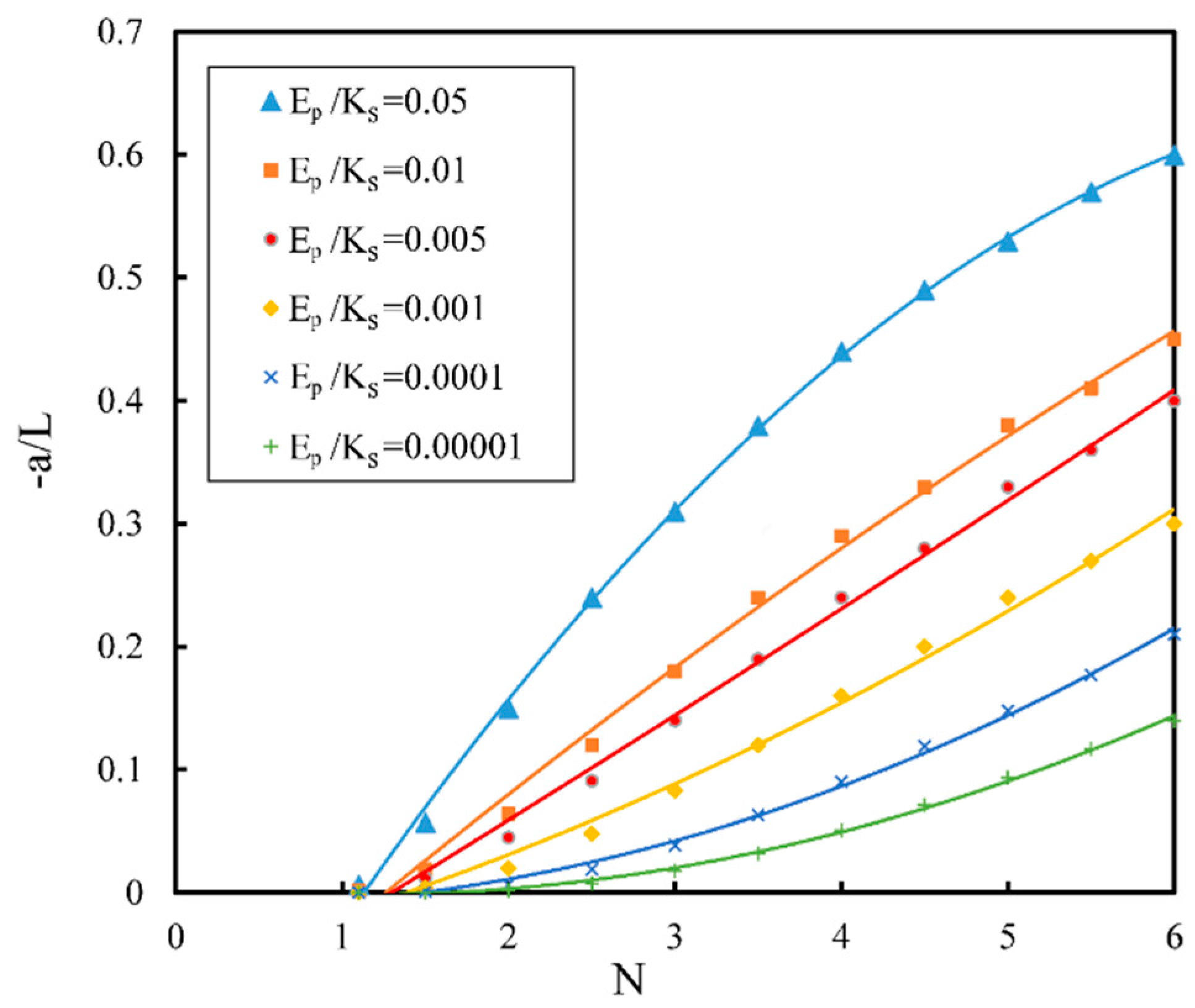
Figure 2.
The evaporation rate (cm/d) calculated by the modified Gardner [23] model and the Brooks–Corey [26] model versus the surface matric potential (-cm) for the Chino Clay (see Table 1). MG and B–C represent the modified Gardner’s [23] model and the Brooks–Corey [26] model in the figure, respectively.

Figure 3.
A comparison of the semi-analytical solutions (solid line) calculated with Equations (18)–(20) using the Brooks–Corey model and the results of HYDRUS-1D simulation (dashed-line) for four soils in Table 4.
Figure 3.
A comparison of the semi-analytical solutions (solid line) calculated with Equations (18)–(20) using the Brooks–Corey model and the results of HYDRUS-1D simulation (dashed-line) for four soils in Table 4.
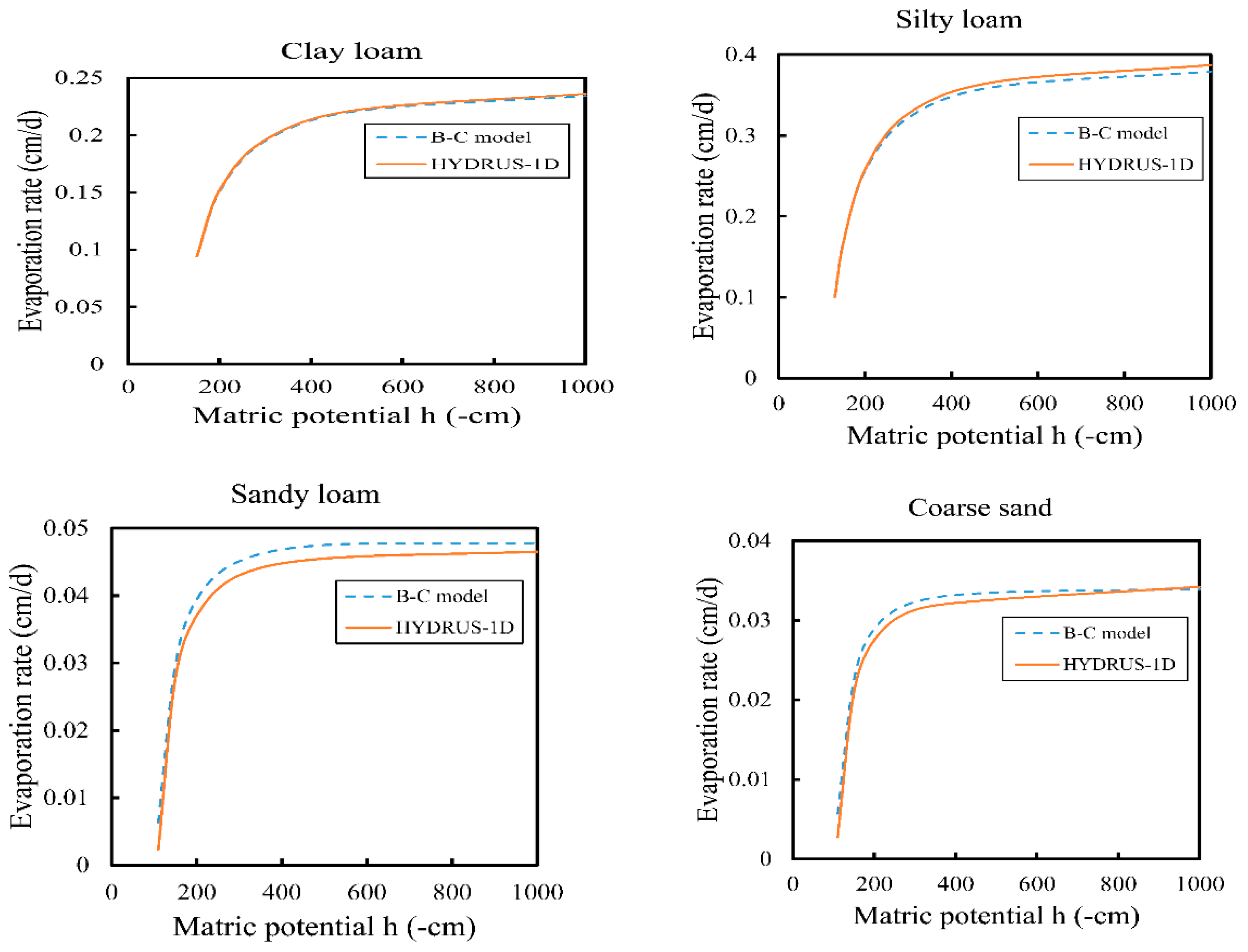
Figure 4.
The ratio between Sadeghi’s solution (denoted as ESSJ where SSJ represents the first letters of last names of three authors of Sadeghi et al. [18]) and our solution of Equations (18)–(20) (denoted as ELZ, where LZ represents the first letters of last names of this paper) for clay loam and 100 cm depth of water table.

Table 1.
Soil parameters used on the modified Gardner model.
| Soil Site/Type | Parameter Value | References |
|---|---|---|
| Chino Clay | N = 2, a = −23.8 cm | [33] |
| Pachappa (fine sandy loam) | N = 3, a = −63.83 cm | [33] |
| Buckeye (fine sand) | N = 5, a = −44.7 cm | [34] |
| Yolo Light Clay | N = 1.77, a = −15.3 cm | [30] |
Table 2.
The Ep/Ks values for different water table depths (L) and soil types.
| L (cm) | 10 | 50 | 100 | 300 | 500 | 1000 |
|---|---|---|---|---|---|---|
| Chino Clay, Ep/Ks | 3.27 | 0.40 | 0.124 | 0.015 | 0.0056 | <0.0001 |
| Pachappa (fine sandy loam), Ep/Ks | 7.07 | 0.96 | 0.280 | 0.016 | 0.004 | 0.00045 |
| Buckeye (fine sand), Ep/Ks | 4.00 | 0.29 | 0.023 | 0.0001 | <0.0001 | <0.0001 |
| Yolo Light Clay, Ep/Ks | 2.38 | 0.29 | 0.096 | 0.014 | 0.006 | 0.002 |
Note: The soil types of this table are the same as those in Table 1.
Table 3.
The discrepancy ratio () of results calculated from Equations (11) and (12).
| E/Ks Soil | 0.05 | 0.01 | 0.005 | 0.001 | 0.0001 | 0.00001 |
|---|---|---|---|---|---|---|
| Buckeye (fine sand) | 17.8% | 3.9% | 2.0% | 0.4% | 0.04% | 0.004% |
| clay loam | 4.8% | 1.0% | 0.5% | 0.1% | 0.01% | 0.001% |
| silty loam | 9.3% | 2.0% | 1.0% | 0.2% | 0.02% | 0.002% |
| sandy loam | 13.6% | 2.9% | 1.5% | 0.3% | 0.03% | 0.003% |
| coarse sand | 13.6% | 2.9% | 1.5% | 0.3% | 0.03% | 0.003% |
© 2017 by the authors. Licensee MDPI, Basel, Switzerland. This article is an open access article distributed under the terms and conditions of the Creative Commons Attribution (CC BY) license (http://creativecommons.org/licenses/by/4.0/).
Share and Cite
MDPI and ACS Style
Liu, X.; Zhan, H. Calculation of Steady-State Evaporation for an Arbitrary Matric Potential at Bare Ground Surface. Water 2017, 9, 729. https://doi.org/10.3390/w9100729
AMA Style
Liu X, Zhan H. Calculation of Steady-State Evaporation for an Arbitrary Matric Potential at Bare Ground Surface. Water. 2017; 9(10):729. https://doi.org/10.3390/w9100729
Chicago/Turabian StyleLiu, Xin, and Hongbin Zhan. 2017. "Calculation of Steady-State Evaporation for an Arbitrary Matric Potential at Bare Ground Surface" Water 9, no. 10: 729. https://doi.org/10.3390/w9100729
Note that from the first issue of 2016, this journal uses article numbers instead of page numbers. See further details here.