Article

An Economic Assessment of the Global Potential for Seawater Desalination to 2050

1
Graduate School of Science and Engineering, Tokyo Institute of Technology, 2-12-1-M1-6 Ookayama, Meguro-ku, Tokyo 152-8552, Japan
2
School of Environment and Society, Tokyo Institute of Technology, 2-12-1-M1-6 Ookayama, Meguro-ku, Tokyo 152-8552, Japan
3
Hydrologic Research Laboratory, Department of Civil and Environmental Engineering, University of California, Davis, CA 95616, USA
4
Center for Social and Environmental Systems Research, National Institute for Environmental Studies, 16-2 Onogawa, Tsukuba, Ibaraki 305-8506, Japan
*
Author to whom correspondence should be addressed.
Water 2017, 9(10), 763; https://doi.org/10.3390/w9100763
Submission received: 25 August 2017 / Revised: 2 October 2017 / Accepted: 2 October 2017 / Published: 6 October 2017

Abstract

:
Seawater desalination is a promising approach to satisfying water demand in coastal countries suffering from water scarcity. To clarify its potential future global scale, we perform a detailed investigation of the economic feasibility of desalination development for different countries using a feasibility index (Fi) that reflects a comparison between the price of water and the cost of production. We consider both past and future time periods. For historical validation, Fi is first evaluated for nine major desalination countries; its variation is in good agreement with the actual historical development of desalination in these countries on both spatial and temporal scales. We then simulate the period of 2015–2050 for a Shared Socioeconomic Pathway (SSP2) and two climate scenarios. Our projected results suggest that desalination will become more feasible for countries undergoing continued development by 2050. The corresponding total global desalination population will increase by 3.2-fold in 2050 compared to the present (from 551.6 × 10⁶ in 2015 to 1768 × 106). The major spread of seawater desalination to more countries and its availability to larger populations is mainly attributed to the diminishing production costs and increasing water prices in these countries under the given socioeconomic/climate scenarios.

1. Introduction

As a valuable basic natural resource that contributes to all societal activities, water is today subject to shortages due to the effects of climate change, economic development, and population growth worldwide [1,2]. To address current and future water scarcity problems, many countries are already engaged in the search for various alternative approaches. For the reasons outlined below, one of these solutions involves the use seawater desalination. First, seawater desalination is totally independent of the natural hydrological cycle, which permits its use in numerous coastal areas. Second, the unit production cost of desalinated water has decreased significantly due to technological progress, and this has resulted in its availability at prices that are competitive with those of some conventional water resources. Indeed, rapid installation of desalination plants has recently been achieved on a global scale, rendering it promising as an adaptation to the effects of climate change on the freshwater supply [3,4].
This study examines seawater desalination that relies on reverse osmosis technology (SWRO) to remove high concentrations of minerals and salts from seawater. RO technology generally requires less total thermal and electrical energy (3–4 kWh/m3) than other conventional commercial desalination technologies, such as multistage flash distillation or multiple-effect distillation (5.5–16 kWh/m3) [3,5,6,7,8]. By 2015, RO technology achieved remarkable gains in the production of desalinated water from seawater (6.9 km3 year−1 of the 12.9 km3 year−1 total global desalinated water production from seawater reported in the DesalData database [9]). As it currently dominates global seawater desalination, SWRO is expected to maintain its trend of growth and to play a greater role in increasing the availability of freshwater in the future.
Numerous previous studies have assessed the future development of seawater desalination based on various scales. Bremere, et al. [10] and Kirshen [11] project the increasing desalinated water volume required for growing domestic or commercial needs to be 2025 year in 10 water-scarce countries and 2050 year in coastal nations, respectively. Additionally, Kim, et al. [12] use an economic approach to predict the growth of total desalinated water as 2100 year at a basin scale. In view of the remarkable development of desalination, efforts have also been made to incorporate desalinated water into various hydrological models for global water resource assessments. For example, Wada, et al. [13] incorporate desalinated water into their hydrological models by allocating its usage in seashore regions and assuming that its volume will increase with the population. Hanasaki, et al. [14] propose a seawater desalination model to identify potential desalination areas and likely production volumes. These studies use reasonable assumptions to predict the development of seawater desalination over various spatial scales. However, little attention has been paid to the local economic conditions of the countries that would potentially use seawater desalination. Thus, further research is needed to examine whether seawater desalination is economically feasible given the specific circumstance of particular countries.
The main economic barrier to implementing seawater desalination derives from its high capital and operational and management (O&M) costs [15]. These will eventually be converted into the price of desalinated water paid by consumers. It is evident that desalinated water will be incorporated as an integral part of a water portfolio once the cost of seawater desalination is reduced to the level that consumers can afford to pay for water resources. Therefore, the feasibility of seawater desalination for different countries is intertwined with two factors: the production cost of desalinated water and the water price, which may be a good proxy for the affordability of water resources. Using various empirical and computerized tools, several existing studies estimate the capital or O&M costs of desalination, as these will directly determine the threshold for building a desalination plant or the long-term operation of a desalination plant [15,16,17,18,19]. However, few studies address the correlation between these two economic factors (i.e., the production cost and water price) when evaluating the development of seawater desalination in different countries.
In this study, we propose a methodology for evaluating the development of seawater desalination and assessing its economic feasibility for different countries over the long term. We develop a detailed feasibility index that involves comparing the water price with the production cost of desalination to determine the feasibility of seawater desalination for each country and to identify the countries that show the economic potential for seawater desalination. Herein, two statistical models for estimating the production cost and water price are outlined; they are discussed in terms of their historical validity (Section 2) as well as their subsequent application to future projections under a Shared Socioeconomic Pathway and two climate policies (Section 3). Based on these projections, we evaluate the feasibility of seawater desalination for different countries and assess the prospects of seawater desalination development in 140 coastal countries by 2050 (Section 3).

2. Materials and Methods

2.1. Data Collection

The parameters adopted in simulations for developing models are shown in Table 1. First, to analyze present desalination capacity, DesalData are primarily used. As of 2014, DesalData included records for more than 17,000 desalination plants. In total, information for the period 1990 to 2014, involving 56 countries, with about 764 SWRO plants, including data on capital cost (EPC-type contracts), plant capacity, location, and contract award year, is analyzed (the detailed criteria and selected countries are summarized in Table S1).
Second, we use socioeconomic data (1990–2014) for the historical simulations based on our models. Socioeconomic data, including the gross domestic product (GDP) and population, are from the database of the World Bank [20]. GDP is analyzed in terms of purchasing power parity (PPP) in 2005 US Dollars. Additionally, the electricity prices for individual countries from 1990 to 2014 are from the IEA database [21]. The municipal water prices for 56 countries from 1990 to 2014 are primarily from Gleick and Michael [22] and the IBNET tariff database [23]. Nationwide water-use data, including water withdrawal and water demand from 1990 to 2000, are from Yoshikawa, et al. [24].
Finally, socioeconomic data from 2015 to 2050 are used for future simulations. As seawater is used as the water resource for SWRO plants, 140 countries, none of which is landlocked, are considered. For the simulation parameters of the GDP (in constant 2005 PPP US Dollars) in these countries, the Shared Socioeconomic Pathway (SSP) Database [25] covering the period of 2015–2050, provided by IIASA, is used. The population is taken from Murakami and Yamagata [26]. Given that different climate policies may impact future energy prices, electricity price data for two climate policies are used. These are from Fujimori, et al. [27]. For the purpose of comparison, all cost figures in this paper are given in 2005 US Dollars, calculated based on the United States Consumer Price Index (CPI).

2.2. Methodology for Assessment of Economic Feasibility of SWRO

In this study, we use one major criterion, whether the cost of produced desalinated water in a given country would be affordable for consumers under local socioeconomic conditions, to examine whether SWRO is economically feasible. At present, approximately ~63% of desalinated water worldwide is used for municipal purposes, 26% is used for industrial purposes, and 6% is used in power stations for electricity generation [29]. As municipalities are the main recipients of desalinated water, the municipal water price is treated as an indicator of the affordability of water resources for consumers.
Here, a feasibility index (Fi) is used to express the potential for implementing SWRO currently or in the future. In detail, Fi is defined as follows:
F i   =   W p C p
where Wp presents the water price ($/m3) in a given country, and Cp is the unit production cost ($/m3) of a SWRO plant at a specific time. When the Fi exceeds the threshold value of 1, this suggests high economic feasibility and great potential for developing SWRO in the given country because desalinated water from SWRO is expected to be affordable for consumers. Thus, to clarify the future potential areas of SWRO, the condition of Fi ≥ 1 can be used to identify the countries where SWRO is promising (i.e., a “country with the potential to develop seawater desalination” (CDSD)). Additionally, we also focus on the population most likely to use seawater desalination, defined as the population living within approximately 165 km of the seashore in each CDSD (hereafter, “desalination population”). To calculate the Fi, two statistical models (i.e., the PC and WP models) are separately developed to estimate the unit production cost and water price in different countries (modeling processes are shown in Section 2.3 and Section 2.4).

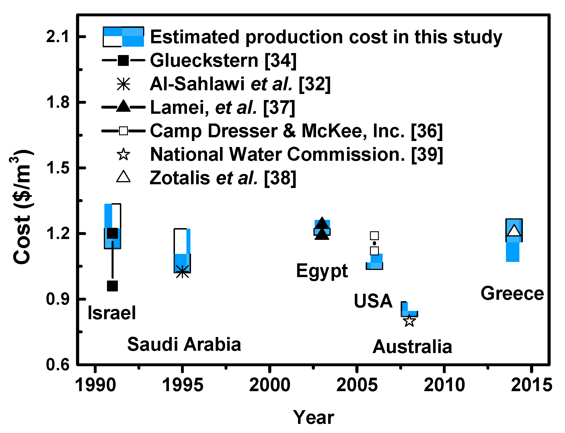
2.3. Statistical Production Cost (PC) Model

The production cost of a SWRO plant can be classified broadly into two major components: capital costs and operation and management (O&M) costs. Regarding the former, the annual amortized capital cost (Ca) can be determined by multiplying the capital cost by an annuity factor, based on the following equation:
C a =   C a p i t a l   C o s t × i × ( 1 + i ) n ( 1 + i ) n 1 ( i   =   8 % ,   n   =   20 )
where Ca is the annual amortized capital cost, the Capital Cost is the initial investment in the starting year, and i and n are the annual discount rates and the SWRO plant life, respectively. We use a discount rate of 8% and a 20-year plant life, which are consistent with a previous study [30].
Furthermore, the annual output of the SWRO plant (capacity) is used to shift the annual amortized capital cost and annual O&M cost (Ca/O&M) to a unit annual amortized capital cost (Cu) and a unit annual O&M cost (CO&M), respectively. As a result, the unit production cost (Cp, US $/m3) for producing 1 m3 of desalted water can be calculated as follows:
C p =   C u   +   C O & M   =   C a C a p a c i t y + C a / O & M C a p a c i t y

2.3.1. Capital Cost Option

To estimate the capital cost of a SWRO plant, it is initially assumed that such a cost would potentially be correlated with four numerical variables (plant capacity (CAP), total installed capacity (TIC), GDP per capita, and distance from the seashore (Distance)) and one dummy variable (Oil-exporting; a value of 1 if the desalination plant is located in one of the top 15 oil-exporting countries, which include Saudi Arabia, Russia, Canada, UAE, Nigeria, Iraq, Kuwait, Angola, Kazakhstan, Venezuela, Iran, Qatar, Mexico, Norway, and Algeria; and 0 otherwise). The rationale for selecting these variables is as follows. As plant capacity directly reflects the size of equipment, the scale of construction, and so on, it will affect the capital cost [16]. The maturity of SWRO technology, reflected in cumulative capacity, is also expected to affect the capital cost [16,31]. In addition to plant capacity and cumulative capacity, Loutatidou, et al. [31] added that whether the desalination plant was located in a country on the Gulf Cooperation Council also has a significant impact on capital cost. Consistent with the literature, the distance from the sea, which may change the investment in transportation, is also included. As the economic level will affect the labor costs, the GDP per capita is expected to change the capital cost. Finally, it is to be noted that ‘Oil-export’ is a dummy variable indicating variations in capital costs in these oil-export countries due to their lower energy costs compared with non-oil-export countries. The authors seek to develop a capital cost function with reference to data for 631 desalting plants built from 1990 to 2002, whereas data for 133 plants from 2003 to 2014 are used to examine the accuracy and availability of developed functions.
The function (f) is estimated by an ordinary least squares method, as follows:
Capital cost = f (CAP, TIC, GDP per capita, Distance, Oil − exporting)
Before estimating the aforementioned function, we tested the multicollinearity among variables as a preliminary step; the results indicate that the variables have little or no correlation with each other (Figure S1 in the Supporting Information). In terms of the quantitative function of capital cost, those variables that result in an improvement in the model fit after their addition are deemed an integral part of the capital cost. We use Akaike’s information criterion (AIC) to check for model accuracy, and the value for each new regressor addition is shown in the Supporting Information (Tables S2–S5). Considering the different characteristics of plants with various capacities, one uniform function may fail to fit all the observed data in an ideal manner. Thus, functions are developed based on the classification of plant capacity in the database, in terms of four groups: A (<1001 m3/d), B (1001–5001 m3/d), C (5001–10,001 m3/d), and D (10,001–900,000 m3/d). Based on the linear regression analysis above, the functional equations for the different capacity groups are calculated as follows:
Capital cost (A) = 2.9 × 10⁶ + 3.3 × 10³ × CAP − 1.9 × 10⁵ × log(TIC) + 1.1 × GDP per capita R2 = 0.98
t-statistic:  (18.9) (156.3)  (−18.9)  (2.5)
Capital cost (B) = 2.1 × 10⁷ + 3.0 × 10³ × CAP − 1.3 × 10⁶ × log(TIC)  R2 = 0.85
t-statistic:  (6.5) (29.3)  (−6.5)
Capital cost (C) = 5.4 × 10⁷ + 2.5 × 10³ × CPA − 3.3 × 10⁶ × log(TIC) R2 = 0.77
t-statistic:  (4.8) (9.6)  (−4.6)
Capital cost (D) = 2.9 × 10⁸ + 1.7 × 10³ × CPA − 1.8 × 10⁷ × log(TIC)  R2 = 0.90
t-statistic:  (4.7) (11.9)   (−4.4)
In Equations (5)–(8), Capital Cost and GDP per capita are in USD, CAP is the plant capacity (m3/year), and TIC is the total cumulative installed capacity of all SWRO plants (m3/year). The t-statistics show that CAP and TIC are significant at the 99% level and that the GDP per capita is significant at the 90% level.
Based on the regression results of Equations (5)–(8), the most statistically significant variables in capital cost estimation are CAP, TIC, and GDP per capita. For the TIC variable, the results suggest that capital cost would decrease with an increase in the total installed capacity. Such a decline could be explained as the result of technological development and the technological learning effect. In cases in which the capital cost continually decreases to an unexpected level over time with an increase in TIC, a minimum threshold vale of $0.15/m3 is used, based on the present minimum value in DesalData. Furthermore, to validate the functions developed in Equations (5)–(8), the function-predicted values of capital cost are plotted against the actual observed values from 2003 to 2014 in Figure S2, with R2 values for each capacity group of 0.98, 0.79, 0.99, and 0.84, respectively. These results suggest a good fit for developed functions and their satisfactory performance in predicting capital costs.

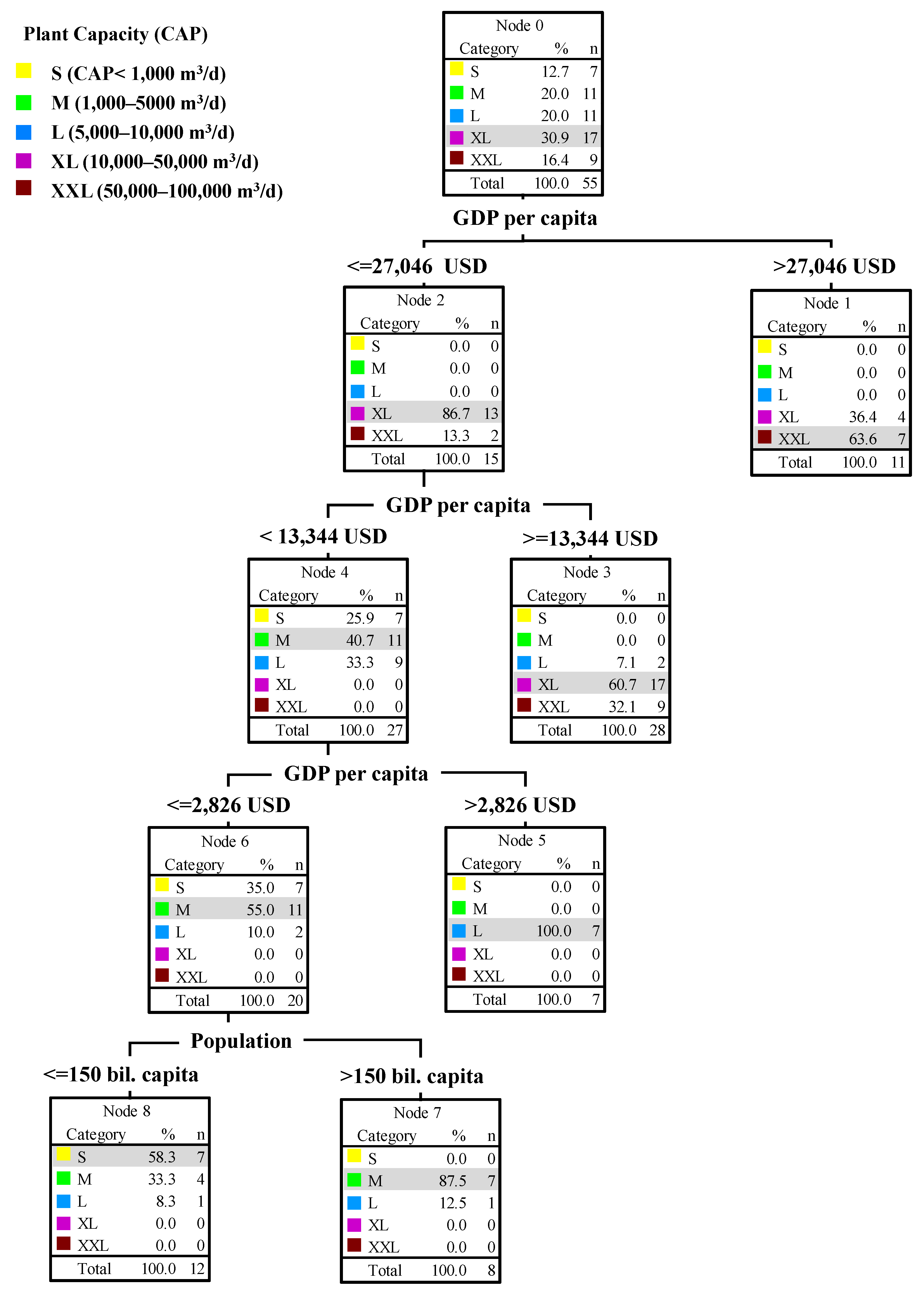
2.3.2. Capacity Option

According to DesalData, even in the same year there are many plants with different capacities installed in one and the same country. Because the variable of capacity plays a significant role in the estimation of unit capital cost, whereas various choices of capacity lead to different estimation results, it is necessary to clarify the capacity selection preference in different countries when a SWRO plant will be built. To that end, a decision-tree model with a Gini index algorithm is typically used to group the target capacity categories within the most homogeneous class. Here, plant capacity choice is classified into five groups: S (capacity of plants <1000 m3/d), M (1000–5000 m3/d), L (5000–10,000 m3/d), XL (10,000–50,000 m3/d), and XXL (50,000–100,000 m3/d). Then, each of these capacity groups is considered as the target category for selection under the splitting variables of GDP per capita and population, denoting the economic and water demand levels in different countries.
This study uses the 88 SWRO plants with the largest capacity installed in each country in different years to build the decision tree and assess its accuracy. As shown in Figure 1, the fitted decision tree includes eight nodes and summarizes the distribution of capacity within each group. For example, in node 3, the proportion of size L is 100%, suggesting that countries with a GDP per capita between 2826 and 13,344 USD PPP/year are more likely to install a SWRO plant of size L. Based on the total distribution of the capacity in different nodes, the data show that countries with higher GDP per capita tend to install SWRO plants with larger capacities. However, when the GDP per capita is less than 2826 USD PPP/year, it seems that the variable of population is more important than the GDP per capita in determining the capacity of a SWRO plant. Finally, to validate the modeled decision trees, a simulated error matrix, described in Table S6 of the Supporting Information, shows that the total accuracy rate of the decision process for correctly attributing locations to the respective actual capacity classes is 64%. The results suggest that the proposed decision tree model is appropriate for simulating capacity selection for different countries, based on their GDP per capita and population.

2.3.3. O&M Cost Option

The unit O&M cost (CO&M) is estimated based on the following economic parameters: maintenance (M), labor (L), membrane exchange (ME), chemical (CE), and energy (ET). These factors cover the general major cost of operating a desalination plant. As a result, the O&M cost can be calculated as follows:
CO&M = M + L+ ME + CE + ET
As the annual unit O&M cost is commonly excluded in DesalData, the values for economic parameters M, L, ME, and CE for use in the abovementioned equation were carefully taken from reports in the literature (Table 1). Indeed, the only uncertain parameter in the O&M cost is the energy cost (ET), which has been shown to be a volatile but significant variable in the calculation of the production cost [5,32]. Electricity is the general required form of energy used by a SWRO plant; thus, the final ET depends on the electricity consumption (kWh/m3) and price ($/kWh). For electricity consumption, it can be assumed to be somewhat uniform over time due to a theoretical barrier [33]. In terms of the price of electricity, we use the price from the national grid, as this is the source for desalination plants in most countries. Based on these results, energy cost is estimated as follows:
ET = PT × fe
where ET is the unit energy cost in US $/m3, PT is the price of electricity in each country (US$/kWh), and fe is the unit electricity consumption of seawater desalination (kWh/m3).
Finally, a historical simulation of the unit production cost (Cp) is performed to validate the summation of unit capital and O&M costs by comparison with previous simulation results [34,35,36,37,38,39]. It should be noted that there is a range of estimated unit production costs in the present study because plant capacity is used as a capacity group from the decision tree. A literature review on unit production cost over time is performed to validate these simulation results. Glueckstern [34] evaluates unit production costs for SWRO plants with 200,000 m3/d capacity and reports a range of $0.96–1.20/m3 in Israel. Al-Sahlawi and Abdulaziz [35] reports a unit production cost of $1.03/m3 for SWRO plants in Saudi Arabia. Additionally, Lamei, et al. [37] estimate a value between $1.19 and $1.24/m3 for plants in Egypt. More recently, the unit production cost of SWRO plants has been placed at between $1.12 and $1.19/m3 in the USA [36]. An even lower value, of $0.8/m3, is reported for unit production costs by National Water Commission [39]. This is based on the estimated results for SWRO plants with a capacity of 208,000 m3/d. Zotalis, et al. [38] estimate the unit production cost for a SWRO in Greece and report a value of $1.21/m3. Our simulation results are fairly consistent with these previous published results for a number of regions and years (Figure 2). This indicates that our PC model satisfactorily estimates the unit production costs of SWROs in different countries based on their individual socioeconomic conditions.

2.4. Statistical Water Price (WP) Model

Generally speaking, the main purpose of water pricing is cost recovery. Depending on the extant policies and socioeconomic conditions, different patterns of water pricing, such as decreasing block tariffs and increasing block tariffs, may be adopted in different countries or areas. For example, a program of decreasing block tariffs, which involves a decrease in the water price as water use increases, is employed only in countries with an abundant water supply, such as Canada [40]. In such countries, water can be considered an economic good, and its price decreases with more consumption due to economies of scales. In contrast, a program of increasing block tariffs, which serves as an incentive for conserving water, is often applied in countries characterized by water scarcity, such as China, India, and Spain [31,41,42]. Therefore, considering the possible differences in the water pricing patterns of countries with different water scarcity indices (the ratio of the water abstraction from a river and the potential water demand [43]), all studied countries are divided into two groups: low water-scarcity countries (water scarcity index > 0.8) and high water-scarcity countries(water scarcity index < 0.8).
In this study, the water price for each group is assumed to correlate with four independent variables (GDP per capita, energy price (electricity price, PT), population density (PD), and water withdrawal per capita (Wpc)). The rationale for the selection of these variables is as follows. As the economic level affects the labor costs in the water supply sector [44], the GDP per capita is used as a main economic parameter to calculate the water price. Additionally, energy costs account for a significant fraction of all operational costs [45]. An increase in energy prices leads to an increase in the production cost of water, which, in turn, leads to an increase in the water price. Thus, the price of electricity is treated as a key factor in the study. Population density is assumed to affect the water price because it can determine the water supply per person, which translates into the average cost for the water supply [46]. Finally, domestic water withdrawal per capita represents the water demand and further reflects the water stress level; hence, it is expected to change the water price [47]. As a result, the treated data set yields the following modeled equation:
Y = β0 + β1Xi1 + ɛi ( i = 1,2,…,m)
where Y denotes the water price (Wp) in a specific country, X denotes each independent variable (i.e., GDP per capita, PT, PD, and Wpc), and β and ε are the weight and error terms, respectively.
For the simulation by a linear regression analysis, we use 105 observed data points representing the water prices in various countries from 1990 to 2010 to establish the function, and the observed data from 2011 to 2014, which include 78 data points, are used to assess the accuracy of the model (modeling processes are shown in the Supplementary Materials, Tables S7–S8.)
The following functions are the results of the linear regression modeling for water prices:
Wp (Low water scarcity countries) =−0.41 + 5.1 × 10⁻⁵ × GDP per capita + 8.0 × PT R2 = 0.67
t-statistic:     (−1.7)   (9.8)   (3.7)
Wp (High water scarcity countries) =−0.06 + 2.7 × 10⁻⁵ × GDP per capita + 4.4 × 10⁻³ × Wpc R2 = 0.64
t-statistic:     (−0.4)   (2.7)   (1.7)
In Equations (12) and (13), GDP per capita is in USD PPP person−1 year−1, and Wpc is the domestic water withdrawal per capita in each country, m3/person. The t-statistics show that GDP per capita and Energy are significant at the 99% level, and Wpc is significant at the 90% level.
To validate these equations, the function-predicted water price, based on the regression analysis, is plotted against the observed actual water price in different countries (Figure S3). The high values of R2 (0.95 and 0.84) indicate the satisfactory performance of the statistical WP model for the estimation of the water price in each country.

2.5. Future Simulations with Developed PC and WP Models

As shown above, the PC and WP models have the capacity to estimate the past unit production cost of SWRO plants and the water price in each country, respectively. Next, these two models are used to project the future unit production cost and water price in different countries over a global scale, assuming that the trends observed over the modeling period (1990–2014) will continue for the next several decades (2015–2050). Attention is focused on the following:
  • Capital cost: Capital cost is estimated using Equations (5)–(8). In these equations, plant capacity selection for each country is based on the results of the decision trees. We assume that each country tends to build the SWRO plant with the largest capacity that is also affordable. For the total installed capacity, Ghaffour, et al. [3] estimate that the current growth rate would be ~55%; here, that same past growth rate is used for the future simulations. Additionally, as in the past simulation, a discount rate of 8% and a 20-year plant life are also used for future periods [30].
  • O&M cost: In both the past and the future periods, labor, membrane exchange, and chemical costs are assumed to be constant, as summarized in Table 1. Equation (10) is used to calculate the energy cost.
  • Water price: The water price is estimated using Equations (12) and (13) for the two scenarios. First, these functions are used to simulate the change in the water price in each country during different years. In our long-term future simulation, the future projected water price is assumed to change uniformly every year. Second, the function, developed based on data from 56 countries, is applied to compute the deficient water price in the other 84 countries that were not included in the observed dataset. For domestic water withdrawal per capita, Hanasaki, et al. [43] estimate that the growth rate would be ~7.3 × 10⁴ m3 person−1 year−1; here, that same past growth rate is used for the future simulations.
  • Socioeconomic condition: Shared Socioeconomic Pathways (SSPs) are newly developed socioeconomic scenarios for use in global climate policy studies. They depict five possible future global situations (SSP1–5). In this study, we perform the future simulations primarily under the SSP2, which involves a middle-of-the road scenario with an intermediate GDP per capita and intermediate population growth. This scenario was selected because it is consistent with the development patterns that have been observed over the past century [48].
  • Climate policy: As mentioned above, energy cost is an integral part of the unit production cost. This may be greatly affected by future climate policies, as different policies lead to different energy prices [27]. In the present study, to clarify the effect of climate policy on future SWRO diffusion, future simulations of PC and WP models are carried out under the following two climate policy scenarios [49]:
    • No climate policy scenario (Baseline): this assumes changes in the socioeconomic conditions in different countries under SSP2 and does not account for the effect of a climate policy (i.e., it assumes there are no constraints on greenhouse gas emissions). Under such a scenario, the energy sources are dependent on traditional fossil fuels.
    • Stringent climate policy scenario (RCP2.6): this assumes changes in the socioeconomic conditions in different countries under SSP2 and accounts for the effect of the stringent climate policy of RCP2.6 (i.e., it assumes a stringent constraint on greenhouse gas emissions aimed at keeping the global mean temperature increase below 2 °C by the year 2100). The RCP2.6 scenarios generally involve more renewable energy resources and a higher carbon tax than does the baseline scenario.

3. Results and Discussion

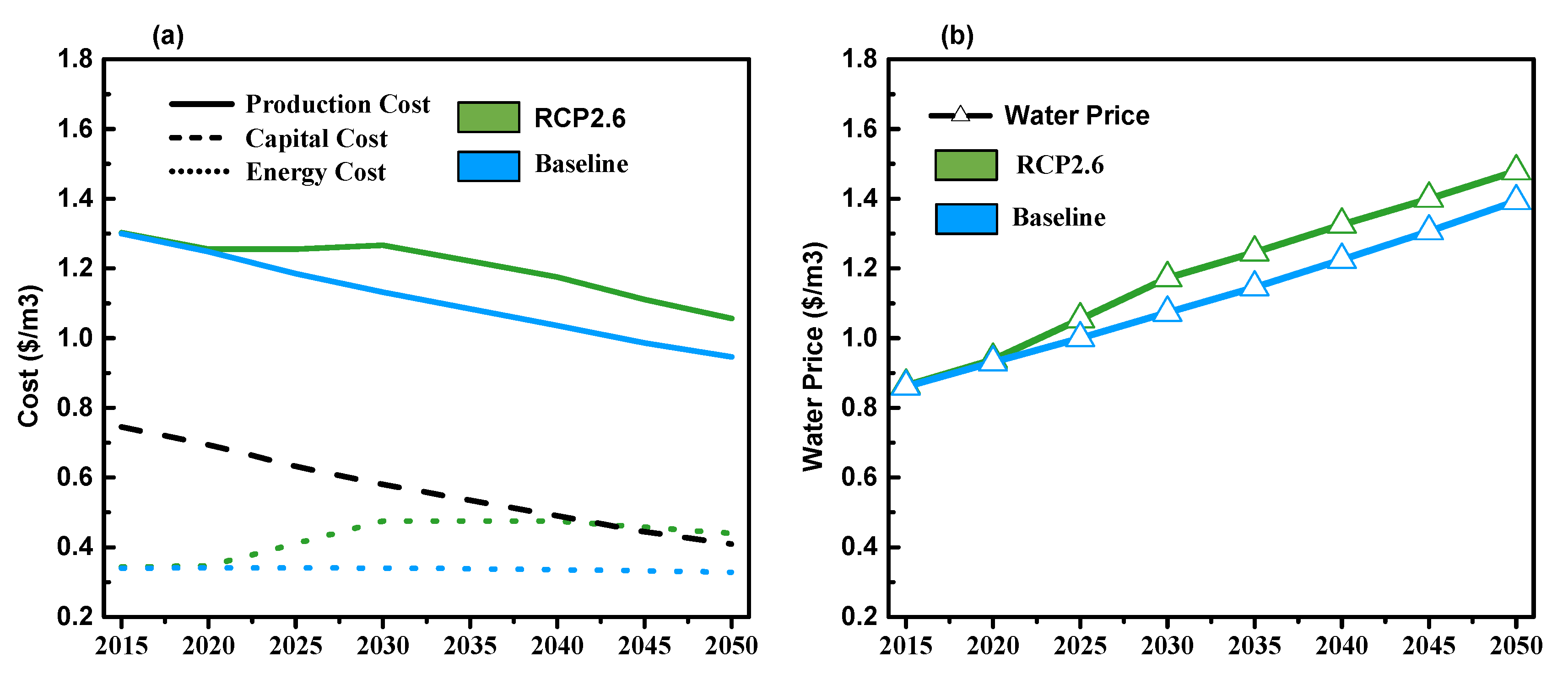
3.1. Production Cost Prediction by Future Simulation of the PC Model

This section focuses on the projection of future unit production costs under each climate policy scenario. Figure 3a shows the projected unit production cost (Cp), unit capital cost (Cu), and unit energy cost (ET) as average values for all studied countries in 2015–2050. Overall, the unit capital cost shows a remarkable decrease, which can be reasonably explained as a result of technological progress and economies of scale, as the increasing of GDP per capita would make it easier to build a SWRO plant with a larger capacity in more countries (Figure S4). By contrast, the unit energy cost increases to some extent as a function of time. This can be primarily attributed to the increase in electricity prices induced by the climate policies within the studied period. This effect is observed in most of the countries studied, especially under the RCP2.6 scenario, as a higher carbon tax is generally imposed as an incentive for reducing greenhouse gas emissions under a more stringent policy. Finally, based on the contradictory contributions of unit capital cost and energy cost to the unit production cost in Figure 3a, the projected average unit production costs over the period of 2015–2050 are expected to be within the ranges of 1.30–0.94 and 1.30–1.1 USD/m3 under the baseline and RCP2.6 scenarios, respectively. These projected unit production costs are industry-wide average levels rather than figures for an individual plant. According to our projections, the unit production cost of SWRO is expected to continue its downward trend within the studied period and to be influenced by different climate policies in that more stringent policies are expected to induce higher unit production costs in most of the studied countries.

3.2. Water Price Prediction According to Future Simulations of the WC Model

We project the water prices in 140 countries over the period 2015–2050 under the baseline and RCP2.6 scenarios. These predicted water prices for all studied countries are further averaged to identify the overall trend with time, and the results are shown in Figure 3b. (The water price for each country is shown on a world map in Figure S5.) Based on the simulation results to 2050, the projected average water price in different countries increases markedly compared with the 2015 figures. The increase in water prices can be attributed primarily to the increased growth of the GDP per capita in most countries under the SSP2, whereas potential changes in the electricity price due to different climate policies probably play a marginal role. Additionally, under the two climate polices, a slightly lower average water price is estimated in each predicted period under the baseline scenario than under RCP2.6 due to the higher electricity price in the latter scenario.

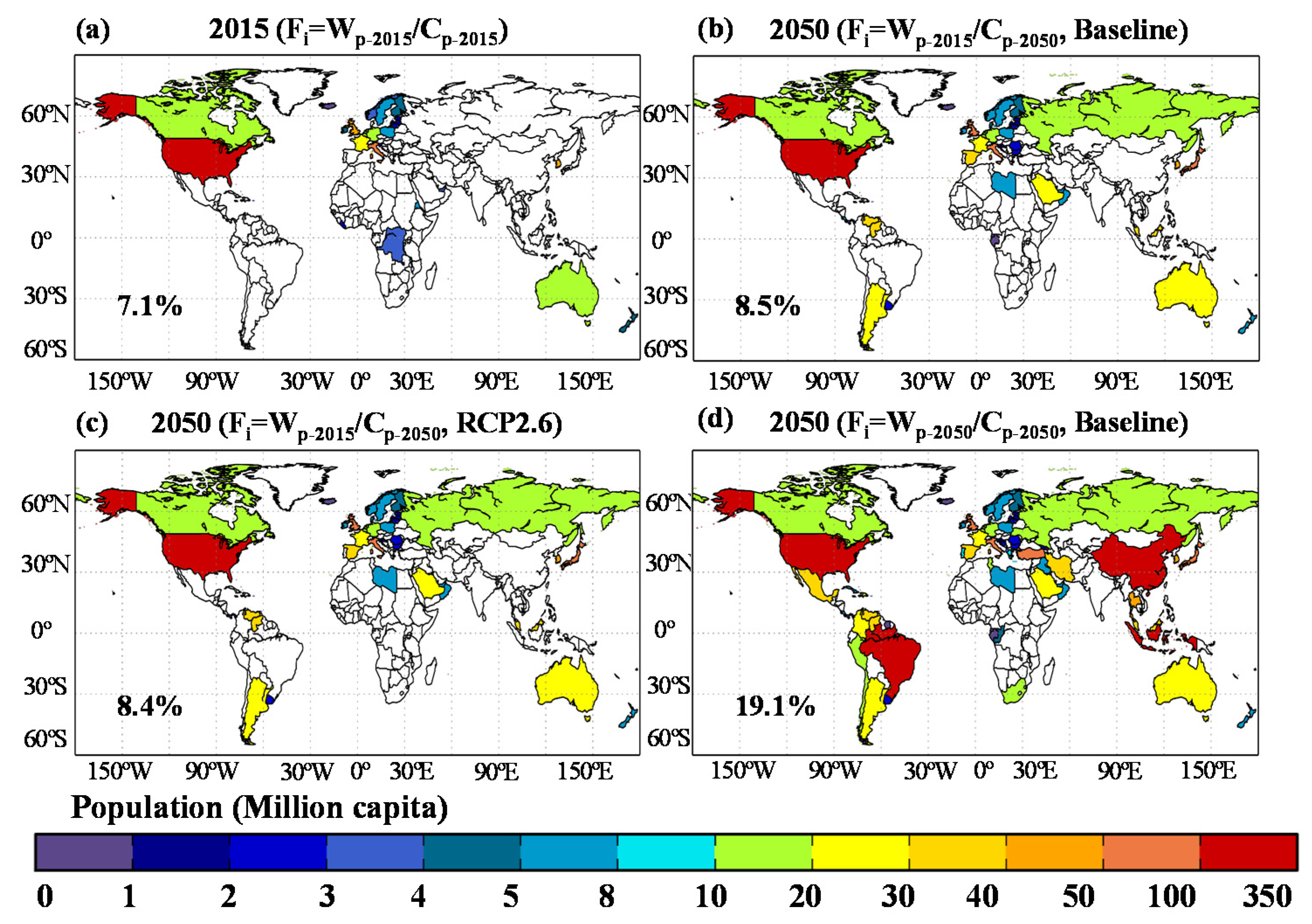
3.3. Economic Feasibility Assessment of SWRO on a Global Scale

First, we perform a historical simulation to validate the feasibility index (Fi) by correlating it with the actual SWRO development in the nine countries (United Arab Emirates, Saudi Arabia, Spain, Kuwait, Israel, Qatar, Bahrain, Oman, and Libya) that dominate global water desalination in terms of reported volume of desalination production [14]. Particular attention is devoted to two aspects: on the spatial scale, we examine whether the Fi for these major countries is consistently higher than its value for the 131 other countries; on the temporal scale, we check whether there is significant long-term consistency between the Fi and TIC for each of these major countries within the studied period. In Figure 4 and Table S9, we summarize the Fi derived from our historical simulation and the TIC in each 5-year interval from 1990 to 2015. Notably, some missing data in each panel are attributed primarily to the limited data for these countries in specific years. As a result, the calculated Fi values for these nine countries range from 0.76 to 4.14 for 2015; these are indeed significantly higher than the values for most of the other countries that account for a negligible proportion of the total global water desalination production (Table S10 in Supplementary Materials). Moreover, for the nine major countries, the data reflect a significant increase in Fi during 1990–2015. This is consistent with the corresponding increase in TIC in these specific years in each of these countries. As a result, the performance of Fi on the spatial and temporal scales suggests that it can be a promising way for assessing the feasibility of desalination because its variability is consistent with the actual historical development of SWRO in major countries. It should be noted that the threshold of the Fi for the application of desalination can be varied for different countries, whereas a standard theoretical value of 1 can contribute to the establishment of a threshold value for the development of SWRO in various countries and thus be used to identify these potential SWRO countries.
Furthermore, based on the future simulated Fi, the next step is to evaluate the economic feasibility of developing SWRO in 140 countries over the period 2015–2050 under the two climate policy scenarios. Specifically, we identify the countries with the potential to develop seawater desalination (CDSDs) and estimate the corresponding desalination population.

3.3.1. Assessment Using the Constant Water Price in 2015

To clarify the effects of unit production cost alone on the future diffusion of SWRO to different countries, we initially use the constant value of the water price in 2015 to calculate the Fi (the Fi for each individual country is summarized in Table S10). Based on the condition of Fi ≥ 1, Figure 5a–c shows the global distribution of the predicted CDSDs and desalination population in each CDSD in different years and under different projection conditions. Table 2 summarizes the total desalination populations in CDSDs for each Fi class. The simulation results identify ~7.1% of global population as the desalination population in 2015 (Table 2). As expected, these desalination populations are distributed primarily in CDSDs, including the most developed nations and oil-exporting countries, especially in North America, Europe, Australia, and the Mediterranean (Figure 5). In the case of the two climate policies, our data show that the total desalination population in all CDSDs increases slightly from 2015 to 2050, to 10.2% and 8.4% of the global population under the baseline and RCP2.6 scenarios, respectively (Table 2). In the RCP2.6 scenario, the increase is less than that in the baseline scenario, and this is primarily attributable to higher energy costs under a more stringent climate policy, as the latter leads to a higher unit production cost of SWRO and a restriction on the diffusion. These results suggest that, without considering the change in water prices, the decline in capital costs contributes to a diminishing unit production cost, rendering the introduction of SWRO in more countries and its application to a greater number of people feasible. However, the increasing unit energy costs caused by various climate policies, especially the more stringent ones, may gradually become a barrier to the further diffusion of SWRO within the studied period. The Paris Agreement sets out an action plan for mitigating global warming below 1.5 °C to reduce the risks of climate change; this is a more stringent target than that included in RCP2.6 in this study. Based on the above-mentioned results, it is expected that the Paris Agreement will, to some extent, limit the future diffusion of SWRO.

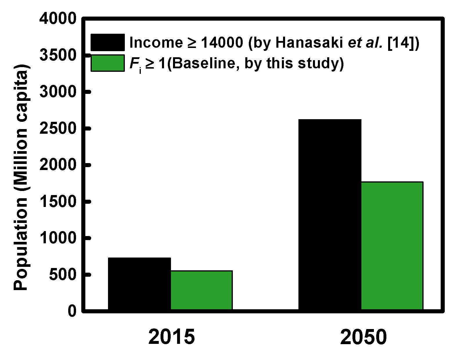
3.3.2. Assessment Incorporating Changes in Water Prices

Next, the change of Fi in 140 countries is estimated based on the binary projected unit production cost and the water price to clarify their synergistic effects on future SWRO development. Figure 5d and Table 2 show the global distribution of predicted CDSDs and the total desalination population in CDSDs in each feasibility index class, respectively. The results highlight two points. First, according to our data, the number of CDSDs in 2050 increases significantly, to 77 versus 34 in 2015, corresponding to 55% of the 140 countries. According to Figure 5d, the range of CDSDs expands to include China, Egypt, Russia, and South Africa, with some countries in South America and Eastern Europe emerging as promising areas for SWRO in the near future. Second, the data show that the total global desalination population in 2050 increases to 1768 × 106 against 551.6 × 10⁶ in 2015, corresponding to 19.1% of the global population. Previously, Hanasaki, et al. [14] set an economic threshold for when the national average GDP per capita exceeds 14,000 USD PPP person−1 year−1 to estimate the spatial extent of where seawater desalination is likely to be used. Their study indicates that the geographical extent of seawater desalination will expand considerably into more non-oil-producing countries, such as Algeria, northern China, and southeastern India, which is consistent with the distribution presented here. Nevertheless, comparison of the populations of these regions that will adopt desalination shows that the criterion of GDP per capita >14,000 USD PPP person−1 year−1 finally leads to a population change from 727 in 2015 to 2619 million in 2050, which obviously exceeds the population change from 551 to 1768 million by the criterion of Fi ≥1 used in this study (Figure 6). This distinction in population is mainly attributed to the fact that our assessment of the future development of SWRO emphasizes its economic feasibility. This involves not only whether building a SWRO plant would be beneficial under local economic conditions but also whether desalinated water would be competitive with other conventional water resources (i.e., whether desalinated water is affordable for consumers).
Two reasons explain the diffusion of SWRO into more countries and its availability to larger populations. One is the diminishing unit production cost, and the other is the increasing water price (Figure 2). Comparison of the significant diffusion of CDSDs in Figure 5d, which is due to the effects of both factors, with the slight diffusion in Figure 5b, which is due to the effects of only production costs, clearly suggests that water price is the main factor determining the future diffusion of SWRO in the studied period.

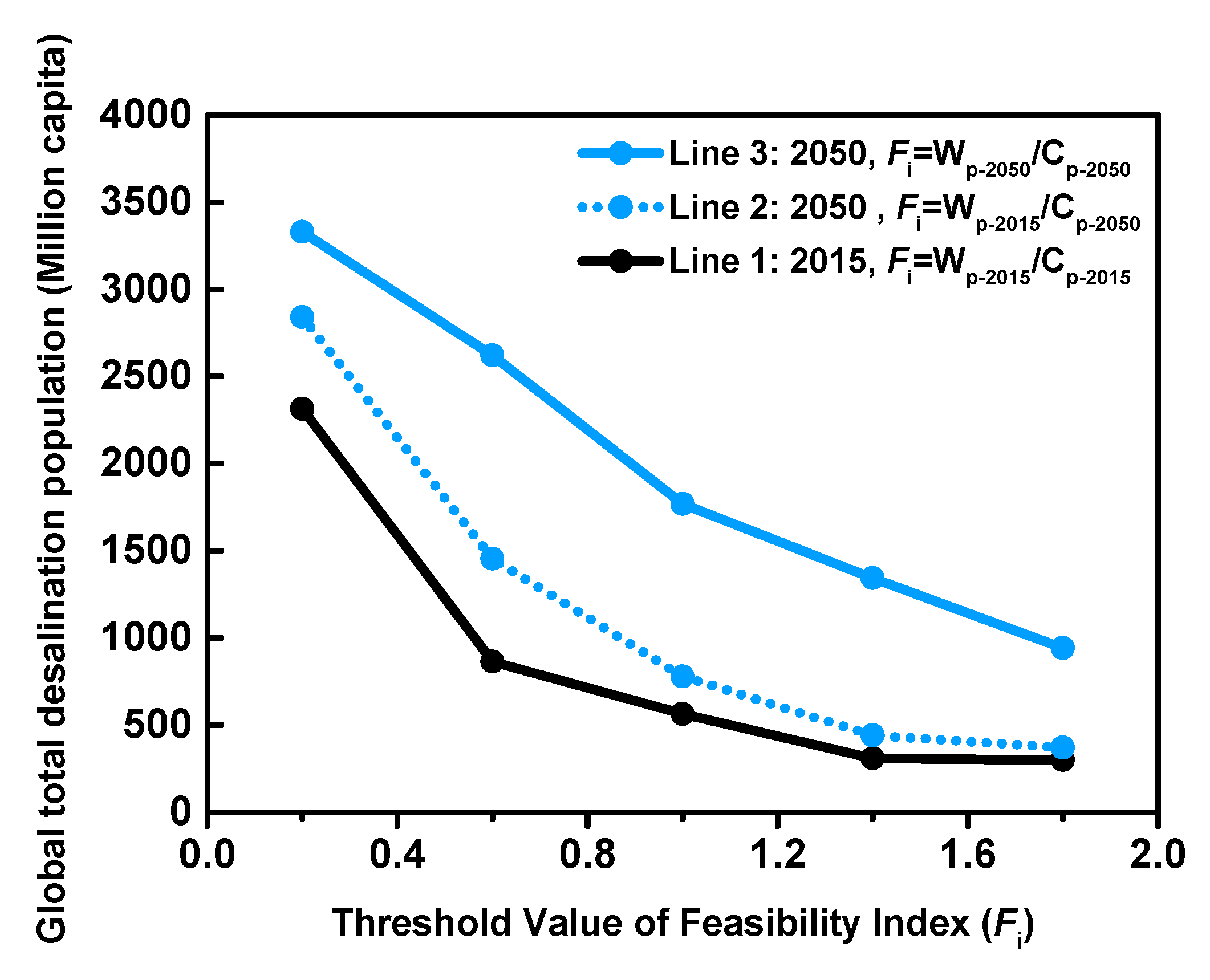
3.3.3. Sensitivity Analysis of the Feasibility Index

The previous sections use 1 as the threshold value of the Fi to identify potential desalination countries and estimate affected populations. However, in reality, different threshold values may significantly affect future simulation results; thus, we conduct a sensitive analysis based on different threshold values of Fi ranging from 0.2 to 1.8.
Figure 7 shows the results of the sensitive analysis. Under all conditions, a higher threshold value of Fi decreases the global total desalination population due to the reduction in the number of CDSDs. For 2015, the data show that the total global desalination population decreases significantly, from 2314 million to 564 million, with a threshold of 0.2 to 1, indicating that desalinated water remains too expensive for most people, leading them to use cheaper water sources. For 2050, the threshold value of Fi ranges from 0.2 to 1.8, and the total global desalination population increases by 1.2–1.7-fold compared to the base year (from 2314–299 million in line 1 to 2840–370 million in line 2) with constant water prices; it increases by 1.4–4.4-fold (from 2314–299 million in line 1 to 3329–943 million in line 3) with changing water prices. These discrepancies between constant and changing water prices suggest the dominant influence of increases in the water price on the future diffusion of SWRO.

3.4. Data Limitations and Uncertainties

Our evaluation of the global economic potential of seawater desalination in this study rests on several assumptions; thus, the limitations of this research should be noted and used as bases for future research.
First, the estimate of the unit production cost of SWRO rests on the following assumptions and is subject to the following limitations. In terms of the capital cost estimates, we assume that investors in each country tend to build SWRO plants with the largest capacity that is affordable. This is based on the reasonable assumption that the capital costs of SWRO plants generally show economies of scale. In reality, the capacities of SWRO plants reflect the total water demand and water use density in each region, which may also be influenced by the availability of cheap electricity; thus, it could be rather diverse, even within the same country. Because our models do not include many detailed design parameters, either unknown or not yet determined, this could render them ineffective. On the other hand, regarding the O&M cost estimate, the waste disposal cost is not included in this study despite the fact that it accounts for a remarkable proportion (3~19%) of the total O&M cost. This is based on the fact that, to some extent, the cost of brine disposal could be partially or fully offset by the profits from selling salt from the desalination by-products [28,29]. Moreover, considering the diversity of the environmental problems of different countries caused by brine discharge and its varied processes, it is nearly impossible to identify a standard quantitative cost of waste disposal.
Second, the assumptions underpinning municipal water price modeling are based on a historical time series analysis, but the limitations of this approach should be considered. We assume a uniform water price for each country, which might be unrealistic. For the same country, even within the same year, Ruester and Zschille [50] report that the prices set by private utilities were higher than the prices set by public utilities when water services were subcontracted out. Although public and private companies may play important roles in pricing, differences within the same country are not considered in the formulation of the water price function due to the limitations of the data.
Finally, the limitations of the feasibility index are summarized. Because water resources are critical to life and economic production, some relatively low-income countries (e.g., Egypt and China) will adopt such technology because of large government subsidies, despite its ostensible lack of economic feasibility. Thus, the Fi threshold may differ among nations, and our model does not include such regional biases. Additionally, although the tradeoff between desalination and other adaptations related to the water supply, such as identifying alternative sources of water or increasing water use efficiencies, may play crucial roles in desalination projects, these mechanisms are not included in the present formulation of the Fi. Finally, in response to unexpected weather events and/or long-term drought in many countries in the world (the US, Australia, Europe), desalination has long been considered a solution to water scarcity. In a drought situation, economic necessity naturally creates demand for desalinated water, regardless of the water price. For example, Spain suffered a severe drought from 1991 to 1995, triggering the rapid construction of major desalination plants. However, when the drought ended and adequate water supplies were available, many users continued to use ‘conventional’ water sources that were then cheaper, and these plants were largely abandoned due to their lack of competitiveness [51]. This kind of investment, which can be seen as temporary, is not included in this study.

4. Conclusions

In this study, the authors propose a method for evaluating the conditions under which it is economically feasible to develop SWRO in 140 countries up to 2050, given a Shared Socioeconomic Pathway (SSP2) and two climate policies. We aim to identify the potential countries and estimate the populations that can economically benefit from SWRO and to clarify the economic determinants of future SWRO diffusion.
First, the authors identify two contributors to the SWRO unit production cost and the municipal water price, which are related reflections of feasibility. Based on the socioeconomic data and modeling techniques, this study specifies common key parameters, develops them into PC and WP models, and demonstrates, via historical validation, that the models can simulate both factors. Second, the developed models are first applied to nine major desalination countries, and the variation in the calculated Fi for those countries is consistent with their actual historical development of SWRO on both the spatial and the temporal scales. Next, using the validated model functions and verified criteria, the unit production cost and water price in 140 countries are separately projected to calculate the Fi under baseline and RCP2.6 scenarios to 2050. Based on the future simulated Fi, the potential development of SWRO is assessed. The results suggest that SWRO would become a more promising approach for countries undergoing additional development by 2050, especially under the baseline scenario. The corresponding total global desalination population will increase by 3.2-fold in 2050 compared to the present (from 551.6 × 10⁶ in 2015 to 1768 × 106). The spread of SWRO into more developing countries and larger populations is mainly attributable to two factors: diminishing unit production costs and increasing water prices. Given the effect of the former factor, the predicted diminishing unit production cost appears to provide a limited driving force for the future diffusion of SWRO because the increasing energy costs caused by stringent climate policies may gradually become a barrier. However, taking both factors into account, we suggest that increasing water prices constitutes the major determinant of the future diffusion of SWRO during the period under examination.
Currently, SWRO is becoming an important practical tool with which to deal with water scarcity in arid countries and satisfy the growing water demand worldwide. The present study is an attempt to evaluate its economic potential, estimate the countries and populations that can most benefit from SWRO from an economic perspective, and clarify the major barriers to its successful diffusion into other countries. The method developed is simple but designed to function with the currently available knowledge base and technology. Despite our assumptions and the limitations of our data, the results suggest general trends in the prospects of SWRO. Our results will be useful for comprehensive projections of the future development of seawater desalination as an integral part of water supply portfolios.

Supplementary Materials

The following are available online at www.mdpi.com/2073-4441/9/10/763/s1. Figure S1: Correlation coefficients between various principle variables to estimate the capital cost, Figure S2: Validation of capital cost, Figure S3: Validation of water prices, Figure S4: Future projections of plant capacity, Figure S5: A world map of the projected water prices, Table S1: Data items and selection criteria, Tables S2–S5: Model’s parameters and performance results of capital cost, Table S6: Error matrix for capacity predictions of SWRO plant, Tables S7 and S8: Model’s parameters and performance results of conventional water price, and Table S9-S10: Feasibility index in past and future simulations.

Acknowledgments

This work was mainly supported by the Japan Society for the Promotion of Science (JSPS) KAKENHI Grant Number JP15H04047 and JP16H06291.

Author Contributions

Lu Gao proposed the methodology of this study; Lu Gao and Shinichiro Fujimori collected the data; Lu Gao analyzed the data and wrote the paper; Lu Gao, Sayaka Yoshikawa, Yoshihiko Iseri, Shinichiro Fujimori and Shinjiro Kanae revised the paper.

Conflicts of Interest

The authors declare no conflict of interest.

References

  1. Oki, T.; Kanae, S. Global Hydrological Cycles and World Water Resources. Science 2006, 313, 1068–1072. [Google Scholar] [CrossRef] [PubMed]
  2. Kundzewicz, Z.W.; Dieter, G. Grand Challenges Related to the Assessment of Climate Change Impacts on Freshwater Resources. J. Hydrol. Eng. 2015, 20, 1943–5584. [Google Scholar] [CrossRef]
  3. Ghaffour, N.; Missimer, T.M.; Amy, G.L. Technical review and evaluation of the economics of water desalination: Current and future challenges for better water supply sustainability. Desalination 2013, 309, 197–207. [Google Scholar] [CrossRef]
  4. Mays, L.W. Groundwater Resources Sustainability: Past, Present, and Future. Water Resour. Manag. 2013, 27, 4409–4424. [Google Scholar] [CrossRef]
  5. Miller, S.; Shemer, H.; Semiat, R. Energy and environmental issues in desalination. Desalination 2015, 366, 2–8. [Google Scholar] [CrossRef]
  6. Schallenberg-Rodríguez, J.; Veza, J.M.; Blanco-Marigorta, A. Energy efficiency and desalination in the Canary Islands. Renew. Sustain. Energy Rev. 2014, 40, 741–748. [Google Scholar] [CrossRef]
  7. Peñate, B.; García-Rodríguez, L. Current trends and future prospects in the design of seawater reverse osmosis desalination technology. Desalination 2012, 284, 1–8. [Google Scholar] [CrossRef]
  8. Al-Sahali, M.; Ettouney, H. Developments in thermal desalination processes: Design, energy, and costing aspects. Desalination 2007, 214, 227–240. [Google Scholar] [CrossRef]
  9. DesalData. Availabe online: http://www.desaldata.com/ (accessed on 5 October 2015).
  10. Bremere, I.; Kennedy, M.; Stikker, A.; Schippers, J. How water scarcity will effect the growth in the desalination market in the coming 25 years. Desalination 2001, 138, 7–15. [Google Scholar] [CrossRef]
  11. Kirshen, P. Adaptation Options and Cost in Water Supply; Tufts University: Medford, MA, USA, 2007. [Google Scholar]
  12. Kim, S.H.; Hejazi, M.; Liu, L.; Calvin, K.; Clarke, L.; Edmonds, J.; Kyle, P.; Patel, P.; Wise, M.; Davies, E. Balancing global water availability and use at basin scale in an integrated assessment model. Clim. Chang. 2016, 136, 217–231. [Google Scholar] [CrossRef]
  13. Wada, Y.; van Beek, L.P.H.; Bierkens, M.F.P. Modelling global water stress of the recent past: On the relative importance of trends in water demand and climate variability. Hydrol. Earth Syst. Sci. 2011, 15, 3785–3808. [Google Scholar] [CrossRef] [Green Version]
  14. Hanasaki, N.; Yoshikawa, S.; Kakinuma, K.; Kanae, S. A seawater desalination scheme for global hydrological models. Hydrol. Earth Syst. Sci. 2016, 20, 4143–4157. [Google Scholar] [CrossRef]
  15. Ziolkowska, J.R. Is Desalination Affordable?—Regional Cost and Price Analysis. Water Resour. Manag. 2015, 29, 1385–1397. [Google Scholar] [CrossRef]
  16. Zhou, Y.; Tol, R.S.J. Evaluating the costs of desalination and water transport. Water Resour. Res. 2005, 41. [Google Scholar] [CrossRef]
  17. Ali, E.S.; Alsaman, A.S.; Harby, K.; Askalany, A.A.; Diab, M.R.; Ebrahim Yakoot, S.M. Recycling brine water of reverse osmosis desalination employing adsorption desalination: A theoretical simulation. Desalination 2017, 408, 13–24. [Google Scholar] [CrossRef]
  18. Caldera, U.; Bogdanov, D.; Breyer, C. Local cost of seawater RO desalination based on solar PV and wind energy: A global estimate. Desalination 2016, 385, 207–216. [Google Scholar] [CrossRef]
  19. Choi, Y.; Cho, H.; Shin, Y.; Jang, Y.; Lee, S. Economic Evaluation of a Hybrid Desalination System Combining Forward and Reverse Osmosis. Membranes 2016, 6, 3. [Google Scholar] [CrossRef] [PubMed]
  20. World Bank. Availabe online: http://databank.worldbank.org/data/home.aspx (accessed on 29 June 2016).
  21. IEA Database. Availabe online: http://www.iea.org/statistics/ (accessed on 9 May 2017).
  22. Gleick, P.H.; Michael, J.C. The world’s Water 2008–2009; Island Press: Washington, DC, USA, 2009. [Google Scholar]
  23. IBNET Tariff Database. Availabe online: https://tariffs.ib-net.org/ (accessed on 27 May 2017).
  24. Yoshikawa, S.; Cho, J.; Yamada, H.G.; Hanasaki, N.; Kanae, S. An assessment of global net irrigation water requirements from various water supply sources to sustain irrigation: Rivers and reservoirs (1960–2050). Hydrol. Earth Syst. Sci. 2014, 18, 4289–4310. [Google Scholar] [CrossRef]
  25. Shared Socioeconomic Pathway (SSP) Database. Availabe online: https://tntcat.iiasa.ac.at/SspDb/dsd?Action=htmlpage&page=about (accessed on 18 October 2016).
  26. Murakami, D.; Yamagata, Y. Estimation of gridded population and GDP scenarios with spatially explicit statistical downscaling. arXiv 2016, arXiv:1610.09041. [Google Scholar]
  27. Fujimori, S.; Hasegawa, T.; Masui, T.; Takahashi, K.; Herran, D.S.; Dai, H.; Hijioka, Y.; Kainuma, M. SSP3: AIM implementation of Shared Socioeconomic Pathways. Global. Environ. Chang. 2017, 42, 268–283. [Google Scholar] [CrossRef]
  28. Kesieme, U.K.; Milne, N.; Aral, H.; Cheng, C.Y.; Duke, M. Economic analysis of desalination technologies in the context of carbon pricing, and opportunities for membrane distillation. Desalination 2013, 323, 66–74. [Google Scholar] [CrossRef] [Green Version]
  29. Ziolkowska, J.R. Desalination leaders in the global market—Current trends and future perspectives. Water Sci. Technol. Water Supply 2016. [Google Scholar] [CrossRef]
  30. Papapetrou, M.; Cipollina, A.; La Commare, U.; Micale, G.; Zaragoza, G.; Kosmadakis, G. Assessment of methodologies and data used to calculate desalination costs. Desalination 2017, 419, 8–19. [Google Scholar] [CrossRef]
  31. Loutatidou, S.; Chalermthai, B.; Marpu, P.R.; Arafat, H.A. Capital cost estimation of RO plants: GCC countries versus southern Europe. Desalination 2014, 347, 103–111. [Google Scholar] [CrossRef]
  32. Al-Karaghouli, A.; Kazmerski, L.L. Energy consumption and water production cost of conventional and renewable-energy-powered desalination processes. Renew. Sustain. Energy Rev. 2013, 24, 343–356. [Google Scholar] [CrossRef]
  33. Semiat, R. Energy Issues in Desalination Processes. Environ. Sci. Technol. 2008, 42, 8193–8201. [Google Scholar] [CrossRef] [PubMed]
  34. Glueckstern, P. Cost estimates of large RO systems. Desalination 1991, 81, 49–56. [Google Scholar] [CrossRef]
  35. Al-Sahlawi, M.A. Seawater desalination in Saudi Arabia: Economic review and demand projections. Desalination 1999, 123, 143–147. [Google Scholar] [CrossRef]
  36. CDM. Water Supply Cost Estimation Study; South Florida Water Management District: West Palm Beach, FL, USA, 2007.
  37. Lamei, A.; Van der Zaag, P.; Von Münch, E. Basic cost equations to estimate unit production costs for RO desalination and long-distance piping to supply water to tourism-dominated arid coastal regions of Egypt. Desalination 2008, 225, 1–12. [Google Scholar] [CrossRef] [Green Version]
  38. Zotalis, K.; Dialynas, E.; Mamassis, N.; Angelakis, A. Desalination Technologies: Hellenic Experience. Water 2014, 6, 1134–1150. [Google Scholar] [CrossRef]
  39. Commission, N.W. Emerging Trends in Desalination: A Review; National Water Commission: Canberra, Australia, 2008. [Google Scholar]
  40. Wilderer, P. Treatise on Water Science; Elsevier Science: Amsterdam, The Netherlands, 2011. [Google Scholar]
  41. McKenzie, D.; Ray, I. Urban water supply in India: Status, reform options and possible lessons. Water Policy 2009, 11, 442–460. [Google Scholar] [CrossRef]
  42. Li, L.; Wu, X.; Tang, Y. Adoption of increasing block tariffs (IBTs) among urban water utilities in major cities in China. Urban. Water J. 2017, 14, 661–668. [Google Scholar] [CrossRef]
  43. Hanasaki, N.; Fujimori, S.; Yamamoto, T.; Yoshikawa, S.; Masaki, Y.; Hijioka, Y.; Kainuma, M.; Kanamori, Y.; Masui, T.; Takahashi, K.; et al. A global water scarcity assessment under Shared Socio-economic Pathways—Part 2: Water availability and scarcity. Hydrol. Earth Syst. Sci. 2013, 17, 2393–2413. [Google Scholar] [CrossRef]
  44. Alexander, Q.; Christine, S.; Kevin, F.; Vanessa, L. National Economic & Labor Impacts of the Water Utility Sector: Technical Report; Water Reserch Foundation: San Francisco, CA, USA, 2014. [Google Scholar]
  45. Linda, J.R. Electricity Use and Management in the Municipal Water Supply and Wastewater Industries; Water Reserch Foundation: San Francisco, CA, USA, 2013. [Google Scholar]
  46. Piper, S. Impact of water quality on municipal water price and residential water demand and implications for water supply benefits. Water Resour. Res. 2003, 39. [Google Scholar] [CrossRef]
  47. Zachariadis, T. Residential Water Scarcity in Cyprus: Impact of Climate Change and Policy Options. Water 2010, 2, 788–814. [Google Scholar] [CrossRef]
  48. O’Neill, B.C.; Kriegler, E.; Riahi, K.; Ebi, K.L.; Hallegatte, S.; Carter, T.R.; Mathur, R.; van Vuuren, D.P. A new scenario framework for climate change research: The concept of shared socioeconomic pathways. Clim. Chang. 2014, 122, 387–400. [Google Scholar] [CrossRef]
  49. Van Vuuren, D.P.; Stehfest, E.; den Elzen, M.G.J.; Kram, T.; van Vliet, J.; Deetman, S.; Isaac, M.; Klein Goldewijk, K.; Hof, A.; Mendoza Beltran, A.; et al. RCP2.6: Exploring the possibility to keep global mean temperature increase below 2 °C. Clim. Chang. 2011, 109, 95. [Google Scholar] [CrossRef]
  50. Ruester, S.; Zschille, M. The impact of governance structure on firm performance: An application to the German water distribution sector. Util. Policy 2010, 18, 154–162. [Google Scholar] [CrossRef]
  51. March, H.; Saurí, D.; Rico-Amorós, A.M. The end of scarcity? Water desalination as the new cornucopia for Mediterranean Spain. J. Hydrol. Part C 2014, 519, 2642–2651. [Google Scholar] [CrossRef] [Green Version]
Figure 1. Decision tree of capacity selection preference for SWRO plants. Each square is a node and is labeled by a node number. In each parent node, a peak and its threshold peak height, used to divide the node into two daughter nodes, are given. For example, in node 1, the peak 13,344 USD PPP/year of GDP per capita was selected. The number (n) of cases in a node and their percentage distribution in the same capacity group are shown in each node frame.
Water 09 00763 g001
Figure 2. Validation of the estimated unit production costs in this study (blue bar, maximum to minimum values) based on comparisons with values from previous studies (dispersed points).
Water 09 00763 g002
Figure 3. Averaged future projections of unit production costs (Cp), capital costs (Cu), and energy costs (ET) for reverse osmosis technology (SWRO) (a) and water price (b) in 140 countries under baseline and RCP2.6 scenarios. Blue, and green, lines indicate baseline and RCP2.6, respectively. Solid, dashed lines, dotted lines, and triangles with solid lines indicate unit production cost, capital cost, energy cost, and water price, respectively.
Water 09 00763 g003
Figure 4. Plot of the total cumulative installed capacity (TIC) against the feasibility index (Fi) in major SWRO countries. The value for each point shows the specific year of the data.
Water 09 00763 g004
Figure 5. Global distributions of the desalination population in each “country with the potential to develop seawater desalination” (CDSD) in different years and under different projection conditions. The values in (ad) show the ratio of the total global desalination populations in all CDSDs to the global population.
Water 09 00763 g005
Figure 6. Simulated total global desalination population in different years under two different standards. Black and green bars show the simulation results using the criteria in Hanasaki et al. [14] and in this study, respectively.
Water 09 00763 g006
Figure 7. Sensitivity analysis of the feasibility index with respect to the total global desalination population for the base year of 2015 (Line 1), 2050 (assuming a constant water price. Line 2), and 2050 (assuming a changed water price, Line 3).
Water 09 00763 g007
Table 1. Socioeconomic parameters and data used in the simulation.
ParameterDataYearRef.
Capital cost56 countries (764 plants)1990–2014[9]
GDP 56 countries1990–2014[20]
Population56 countries1990–2014[20]
Electricity56 countries1990–2014[21]
Water price56 countries1990–2014[22,23]
Water withdrawal56 countries1990–2000[24]
Water demand56 countries1990–2001[24]
For future period
GDP 140 countries2015–2050[25]
Population140 countries2015–2050[26]
Electricity17 Regions2015–2050[27]
Economic Parameters
Labor cost0.1 US $/m3 [15]
Chemical cost0.07 US $/m3 [15]
Membrane exchange cost0.03 US $/m3 [15]
Energy consumption4 kWh/m3 [6]
Maintenance cost2% of capital cost [28]
Table 2. Total global desalination population and percentages of global population in each feasibility index class in different years and under different projection conditions.
BaselineRCP2.6Baseline
(Fi = Wp-2015/Cp-2015)(Fi = Wp-2015/Cp-2050)(Fi = Wp-2015/Cp-2050)(Fi = Wp-2050/Cp-2050)
2015205020502050
ClassPopulationPercentPopulationPercentPopulationPercentPopulationPercent
(Million)(Million)(Million)(Million)
1 (Fi < 0.5)1086.814%1622.218%1695.419%610.47%
2 (0.5 < Fi < 1)382.95%995.711%929.110%1018.111%
3 (1 < Fi < 2)358.45%411.14%410.14%1238.814%
4 (2 < Fi < 4)193.22%364.54%361.94%514.96%
5 (4 < Fi < 7)0.00.0%3.10.0%0.00.0%14.30.2%
Global population7811.3 9149.4 9149.4 9149.4
Class > 2551.67.1%778.68.5%771.98.4%1768.019.3%

