Three-Dimensional Modeling of Wind- and Temperature-Induced Flows in the Icó-Mandantes Bay, Itaparica Reservoir, NE Brazil


1
Chair of Water Resources Management and Modeling of Hydrosystems, Technische Universität Berlin, Gustav-Meyer-Allee 25, 13355 Berlin, Germany, [email protected]
2
Chair of Water Quality Control, Technische Universität Berlin, Straße des 17. Juni 135, 10623 Berlin, Germany
*
Author to whom correspondence should be addressed.
Water 2017, 9(10), 772; https://doi.org/10.3390/w9100772
Submission received: 8 August 2017
/
Revised: 27 September 2017
/
Accepted: 30 September 2017
/
Published: 10 October 2017
Abstract
:The Icó-Mandantes Bay is one of the major branches of the Itaparica Reservoir (Sub-Middle São Francisco River, Northeast Brazil) and is the focus of this study. Besides the harmful algae blooms (HAB) and a severe prolonged drought, the bay has a strategic importance—e.g., the eastern channel of the newly built water diversion will withdraw water from it (drinking water). This article presents the implementation of a three-dimensional (3D) numerical model—pioneering for the region—using TELEMAC-3D. The aim was to investigate the 3D flows induced by moderate or extreme winds as well as by heating of the water surface. The findings showed that a windstorm increased the flow velocities (at least one order of magnitude, i.e., up to 10−1–10−2 m/s) without altering significantly the circulation patterns; this occurred substantially for the heating scenario, which had, in contrast, a lower effect on velocities. In terms of the bay’s management, the main implications are: (1) the withdrawals for drinking water and irrigation agriculture should stop working during windstorms and at least three days afterwards; (2) a heating of the water surface would likely increase the risk of development of HAB in the shallow areas, so that further assessments with a water quality module are needed to support advanced remediation measures; (3) the 3D model proves to be a necessary tool to identify high risk contamination areas e.g., for installation of new aquaculture systems.
1. Introduction
Managing reservoirs in the semi-arid region of the Brazilian Northeast is becoming dramatically challenging. The severe drought affecting the area since 2012 increased the conflicts among the multiple uses of water and it demands urgently more efficient communication and coordination between the different water users [1,2]. The prolonged dry periods predicted by climate change models are expected to reduce the dilution of nutrients and contaminants and affect the ecosystem by increasing water temperatures and reducing oxygen saturation levels; therefore, more eutrophic conditions are expected in lakes [3]. Phenomena such as droughts and the occurrence of harmful algae blooms (HAB) are increasingly affecting water bodies, especially those located in semi-arid areas [4,5]. Additionally, climate change effects influence the trophic level of lakes through many processes such as water heating, enhanced primary production and promotion of cyanobacteria by a high radiation input and intensification of bioremediation with decreased oxygen concentrations. In the region, further ecosystem impacts are generally attributed to the intensive and increasing aquaculture production, by the insufficient treatment of sewage from agricultural villages and by the untreated drainage water from irrigation [5]. Due to the decreasing inflows and the warming climate, the number of reservoirs with water quality problems is likely to increase in semi-arid regions of the world [6]. The high nutrient and sediment loads due to human activities and wastes, enhanced by soil leaching and wash-out during tributaries’ flash floods, lead to more extensive and/or rapid eutrophication in reservoirs, compared to natural lakes [6,7,8].
Finding climate change-adaptive solutions to manage multiple uses of water through innovative technologies, as well as stakeholder procedures, will promote sustainable economic development in Brazil. This was the general aim of the INNOVATE project, to which this work belongs. The binational and interdisciplinary research project provided scientific research in the São Francisco River Basin and improved opportunities transferable to other hydropower reservoirs in semi-arid areas [2]. Adaptive management measures must be developed to mitigate the environmental impacts on reservoirs, primarily greenhouse gas emissions, eutrophication and water level fluctuations, among others [2,5,9].
Computational Fluid Dynamics (CFD) models are widely used to simulate complex hydrodynamics and transport (e.g., sediment) in various natural systems. Such models also allow to examine the effects of particular factors, and thus, identify research needs [10]. Models can be powerful tools to conceptualize complex interactions in natural resource management and to develop appropriated policies, supporting a systematic, integrative and multidisciplinary assessment at various scales [11]. Understanding and communicating the causal connections between fate and effects is fundamental for public acceptance of legislative steering to responsibly compromise between the use of water resources and the conservation of their ecological status therefore advanced numerical tools are required [12].
For instance, Fenocchi et al. [13] investigated the effects of wind and complex bathymetry, comparing a 2D shallow water solver and a 3D Reynolds-averaged Navier-Stokes one, for the Superior Lake of Mantua, a shallow fluvial lake in Northern Italy. De Marchis et al. [14,15] used the 3D finite volume model PANORMUS [16], to assess wind- and tide-induced currents in the Stagnone di Marsala Lagoon and in the Augusta Bay in South Italy. The thermal stratification patterns using hydrodynamic modeling tools for water bodies in semi-arid areas were investigated by Abeysinghe et al. [17] with the aim to prevent algae blooms and eutrophication processes in the Kotmale Reservoir, Sri Lanka. They used a self-developed one-dimensional numerical model, called DYRESM, to predict the distribution of temperatures in response to meteorological forcing, inflow and outflow. Liebe et al. [18] focused their work on some small reservoirs located in Africa (Ghana, Burkina Faso, Zimbabwe) and in Brazil, with the aim to assess their impacts on the rural communities, and thus, stimulate the improvement of water availability and economic development through proper planning, maintenance and operation. Abbasi et al. [19] assessed the heat exchange processes and the temperature dynamics between water and air in the small Lake Binaba in Ghana, as a tool to identify the impacts on water quality, enabling biological and environmental predictions.
Two- (depth-averaged) and three-dimensional (2D and 3D, respectively) models are usually preferred for lakes and reservoir management and the choice between them depends on whether the vertical variability of velocities, tracer profiles and stratification are significant or not. Nevertheless, one-dimensional (vertical) numerical models are also often applied for lakes, with the main purpose to assess eventual stratification patterns and temperature profiles over the water depth. For instance, Ladwig et al. [20] coupled the 1D-vertical General Lake Model (GLM) with the water quality AED2 to study wind-induced flow and nutrients spreading in the Lake Tegel in Berlin. In general, physical forces induce 3D effects on the flow field; forces applied on the free surface of a water body are transferred at depth by turbulence in the vertical plane; thus, the depth-averaged approximation is generally more limiting for wind-driven flows than for gravity-driven ones, such as straight rivers [13]. Wind in the first place, but also temperature changes affect hydrodynamics and water quality [19]. In particular, local scale analyses are connected to macrophytes and wind mixing, as well as to the transport of nutrients and pollutants across reservoirs [21,22]. The usefulness of 2D models is restricted to processes associated to the horizontal circulation, disregarding precise advection time scales and flow paths at specific depths [13]. In the case of large lakes, the assumption of horizontal uniformity is rarely valid, hence the application of 3D hydrodynamic models is required for proper calculations, as pointed out by many researchers even for very shallow depths (e.g., [14,19]).
Within the framework of the above-mentioned INNOVATE project, this study focuses on the Icó-Mandantes Bay, one of the major branches of the Itaparica Reservoir (Pernambuco, NE Brazil). Although in many regions, small inland water bodies act as multi-purpose water sources, being extremely important for economic development, improving smallholder livelihoods and food security, hydrological impact assessments are rarely carried out [18]. In the study area, no modeling studies were found in literature and urgent questions have been raised in the last years by water managers, such as the effects of the newly built water diversion project on water quantity [23] or the impacts on water quality of the net-cage-based aquaculture systems, increasingly developing in the reservoir [24]. To answer to such stakeholders- and issues- oriented demands, in previous research [25,26,27], a 2D model capable to simulate hydrodynamics and tracer transport was setup and tested for several scenarios, using the open-source software TELEMAC-MASCARET [28]. The main hydraulic outcomes were that the water exchange between the Icó-Mandantes Bay and the reservoir main stream was hardly occurring, since the water in the bay is almost stagnant, in absence of external forces such as wind or flood events. Therefore, the same water body can be characterized by different flow (and vertical eddy viscosity) regimes [25,29]. Important management suggestions have been given in that context, for example in regards to the urge of assessing the spreading of contaminants in the domain, introduced for instance by the harmful flash floods occurring from the intermittent tributary Riacho dos Mandantes, located next to the withdrawals for water supply [27].
So far, the vertical flows (3D effects) induced by wind and temperature have not yet been taken into account in the Icó-Mandantes Bay. Only a limited number of CFD simulations for temperature distribution in shallow and small inland water bodies in semi-arid areas can be generally found [19]. As addressed by numerous experts [6,12,15,19], weather conditions (wind, temperature) influence currents and stratification in reservoirs, whose hydrodynamic processes and thermal state are the main drivers of their ecosystem. The classification of lakes according to their circulation patterns has proven to be very useful for limnology assessments [12,30]. Moreover, the vertical resolutions of the measured temperature profiles are often not sufficient for assessing small-scale turbulence effects or investigating variations of water temperature induced by wind velocity and heating in shallow waters [19]. Therefore, research is needed to deepen the knowledge of such complex processes in areas already challenged by climate change, water multiple uses and lack of advanced modeling techniques. In this article, the setup of a 3D model for the Icó-Mandantes Bay is presented, as well as the implementation of scenarios investigating hydrodynamics, wind- and density-induced flows. The study focuses on the 3D effects caused by wind and temperature changes over the vertical water column, addressing the following research questions:
- Since wind is considered responsible of hydrodynamic mixing in water bodies and of the relevant increase of flow velocities during storms in shallow lakes [13,15], does the wind (moderate wind, windstorms) significantly influence the three-dimensional flow circulations also in the Icó-Mandantes Bay and in which way? How do the flow velocities change and to which extent?
- Density differences are known to drive currents [6,12,19,21]: how does heating of the water surface due to warmer air temperature alter the hydraulics in the bay and how (e.g., velocity profiles, intensities)? Which are the consequent three-dimensional effects (e.g., stratification, flow circulation)?
- In the revised literature, the implications of the numerical results for appropriate environmental policy and management are often not explored and the focus of discussion is strictly limited on the hydrodynamic findings. In contrast, we intend to additionally address in this work: how do the outcomes of this research influence management of the bay (sustainability of aquatic ecosystem services)? Which are the recommendations and the adaptive measures to be embraced?
The results of this work deepen the knowledge of the complex hydrodynamics of this bay or similar behaving small water bodies in semi-arid areas, being particularly useful for future modeling studies, for stakeholders and water managers, in order to save time and resources.
2. Governing Equations
The hydrodynamics and transport simulated in the Icó-Mandantes Bay are solved through the three-dimensional shallow waters equations at each time step and in each point of the mesh [28]. For this case study, a free surface changing in time, an incompressible fluid, the hydrostatic pressure hypothesis and the Boussinesq approximation for the momentum were assumed [28,31]. The equations governing the flow are the continuity equation—i.e., the conservation of the fluid mass—and the momentum equations in x-, y- and z-directions. The latter consists of the simplified equation for the vertical velocity w, given to the hydrostatic pressure hypothesis, which considers the pressure at one point depending on the atmospheric pressure on the surface and on the weight of the column of water above it.
The wind shear stresses ( and , in x- and y-direction, respectively) were determined in function of the wind speed at 10 m height ( [m/s]), the density of the air ( [kg/m3]) and a dimensionless empirical coefficient (), calculated according to the formula used by the Institute of Oceanographic Sciences (United Kingdom) [28], reported in Equations (1) and (2):
where and [m/s] are the components of wind velocity in x- and y-directions. The information about wind values used in the simulations are given in Section 4.2.
No flow measurements were available in the study area therefore a proper calibration and validation for velocities, concentrations and temperatures could not be conducted. Values calibrated in previous work for the same reach under study and for similar flow discharges [32] have been used for the Strickler coefficient to evaluate the bottom friction, assuming it equal to 30 m0.33/s. Additionally, values of bottom friction were varied in the range between 25 and 35 m0.33/s and the results showed very small differences. Such values for friction are standard values for the type of soil and system of the bay under study.
Simple turbulence models were applied for the horizontal and vertical directions, which are respectively the constant viscosity and the mixing length Prandtl model [28,31], giving nearly same results as more complex models (e.g., k-ε) computed for a defined reference case under same conditions (e.g., checking mass conservation, velocities and water depths). Additionally, when running the k-ε model for the simulations, TELEMAC computes the turbulent viscosity coefficient for the specific scenario (horizontal and vertical). The results of the sensitivity studies conducted concerning the turbulent viscosity (10−2 ÷ 10−6 m2/s; the latter is the TELEMAC default value) did not show high sensitivity to such parameters. Thus, the horizontal viscosity νt,th was assumed equal to 10−4 m2/s for each case, which is in the range of literature values and of the results obtained with the k-ε model.
The governing equation of the tracer transport is reported in Equation (3), which consists of the heat transport equation, where the turbulent diffusivity was set equal to the turbulent viscosity of the momentum equations [28,33].
where [°C], [kg/m3] represent the water temperature and the water density and are calculated by the model; , [m2/s] are the horizontal and vertical turbulent thermal diffusivity.
The density-induced flow computed by the equation of state established by UNESCO [28] is:
where [kg/m3] is the reference water density and [°C] is the reference water temperature. The water density [kg/m3] is function of the water temperature , assuming here that it is in the range of 0 to 40 °C.
According to Hervouet [28] and Sweers [34], the boundary condition at the water surface is:
where [°C] is the atmospheric temperature; [J/kg/°C] is the specific heat equal to 4.18 and [W/m2/°C] is the so-called exchange coefficient. Equation (5) assumes that the thermal power exchanged between water and atmosphere per surface unit is proportional to the temperature gradients between water and air by the exchange coefficient [W/m2/°C]:
where the parameter [-] depends on the location of the study area: 0.0025 was chosen, average suggested by [28] for regions near the Atlantic shores. The exchange coefficient is the result of the nomogram developed by Sweers [30], which relates at the water-air interface to the wind speed and the surface temperature, approximating the phenomena like radiation, convection of air in contact with water and latent heat produced by water evaporation.
3. Study Region
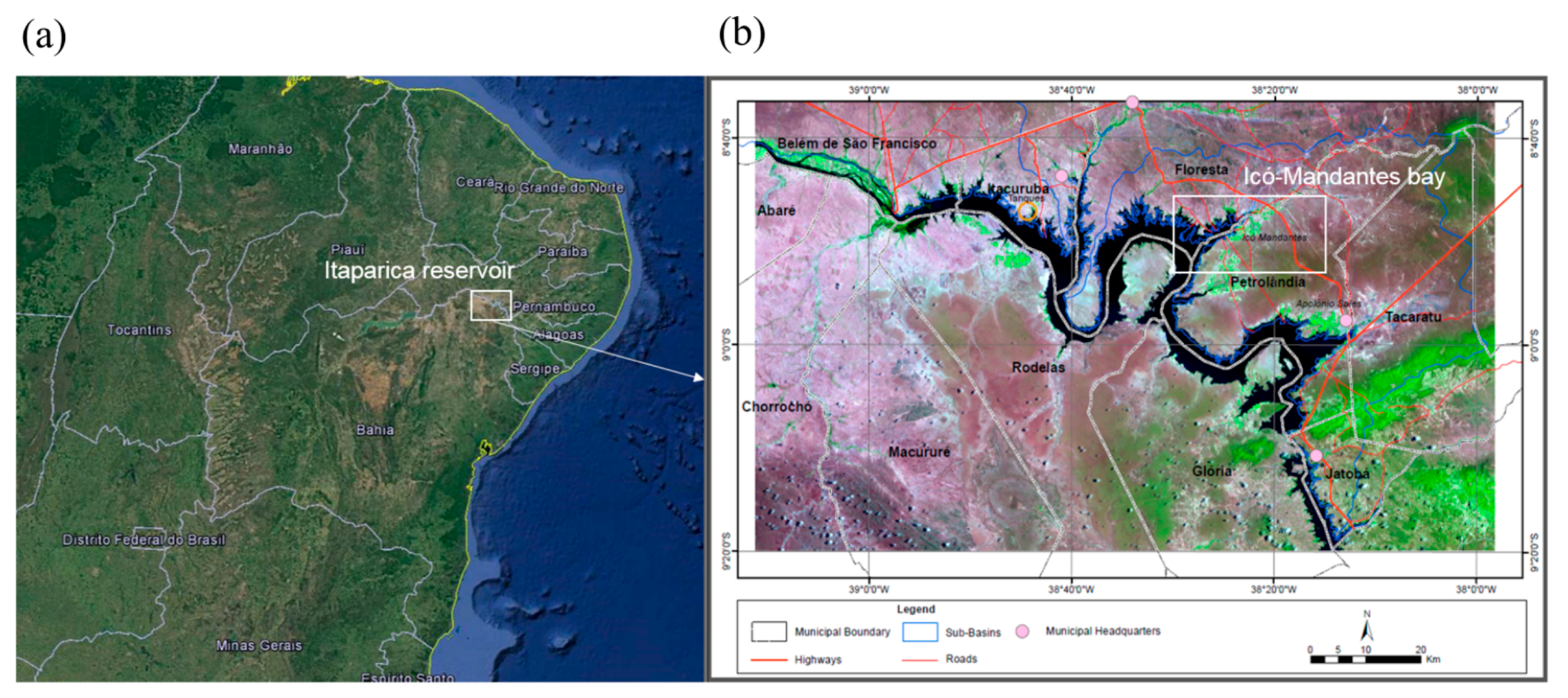
The area of interest is the Icó-Mandantes Bay, one of the major off-stream branches of the Itaparica Reservoir, located in the semi-arid state of Pernambuco, NE Brazil (Figure 1). The reservoir is formed by the Luiz Gonzaga dam, built in the late 80 s, in the Sub-Middle São Francisco River. The mean water discharge is 2060 m3/s, regulated by the upstream Sobradinho Reservoir, and the mean water elevation 302.8 m a.s.l., with a maximum annual water level fluctuation of maximum 5 m [35]. The average and the maximum water level of the reservoir are respectively 13 m and 42 m [2].
The morphometric, chemical and limnological characteristics of the Icó-Mandantes Bay have been presented in detail in [24,36,37,38]. The study area has high air temperatures and strong winds concentrated in some hours of the day. The bay is vertically mixed, it has low water conductivity and low nutrients loads, which increase significantly during flash floods from the tributaries. The mean annual precipitations of ~475 mm/y are usually occurring between January and April during rare intense events. Between 2012 and 2015, the median water quality of the Itaparica Reservoir is characterized by low conductivity (71 µS/cm) and low nutrient concentrations (dissolved inorganic nitrogen = 98 µg/L, total phosphorus = 20 µg/L), a transparency of 2.3 m Secchi disk depth and Chlorophyll a = 1.7 µg/L; thus, the reservoir was classified as mesotrophic. The water quality in the Icó-Mandantes Bay is depleted by an intermittent river inflow (called Riacho dos Mandantes) with high short-term nutrient input during the rainy season and by the drainage channels of the irrigated agriculture areas, located in the southeastern part of the bay. After such strong rain events, the median nutrient concentrations changes relevantly, with dissolved inorganic nitrogen = 77 µg/L, total phosphorus = 34 µg/L, a transparency of 0.9 m Secchi depth, and Chlorophyll a = 38 µg/L [39]. Nearly 35 to 45% of the bay area is covered by a submerged weed, namely Egeria densa. Due to the water level fluctuations caused by hydropower use—in particular when the surface elevation decreases—these dense vegetation mats are another significant source of nutrient input for the bay, after desiccation and mineralization [36,38]. Among others, such undesired effects due to declining lake levels were also observed by Zamani in the Abolabbas Reservoir, Iran [6].
Nowadays the uses of the Itaparica Reservoir are many—besides the water storage and energy generation, it is also used for irrigation agriculture and aquaculture production, human and animal water consumption, navigation, recreation and fisheries. In particular, the Icó-Mandantes Bay is strategic for the local water management for numerous reasons. The eventual future development of new aquaculture systems in the bay of the reservoir may increase the phosphorus contents and the potential for eutrophication [24,26]. Water withdrawals for human and animal supply, as well as for irrigation agriculture, occur in the bay, where also the newly built water diversion channel (Figure 2) will operate with the aim to divert water to into the even drier northern watersheds [27].
4. Setup of the Model and the Scenarios
4.1. Computational Domain and Processing Tools
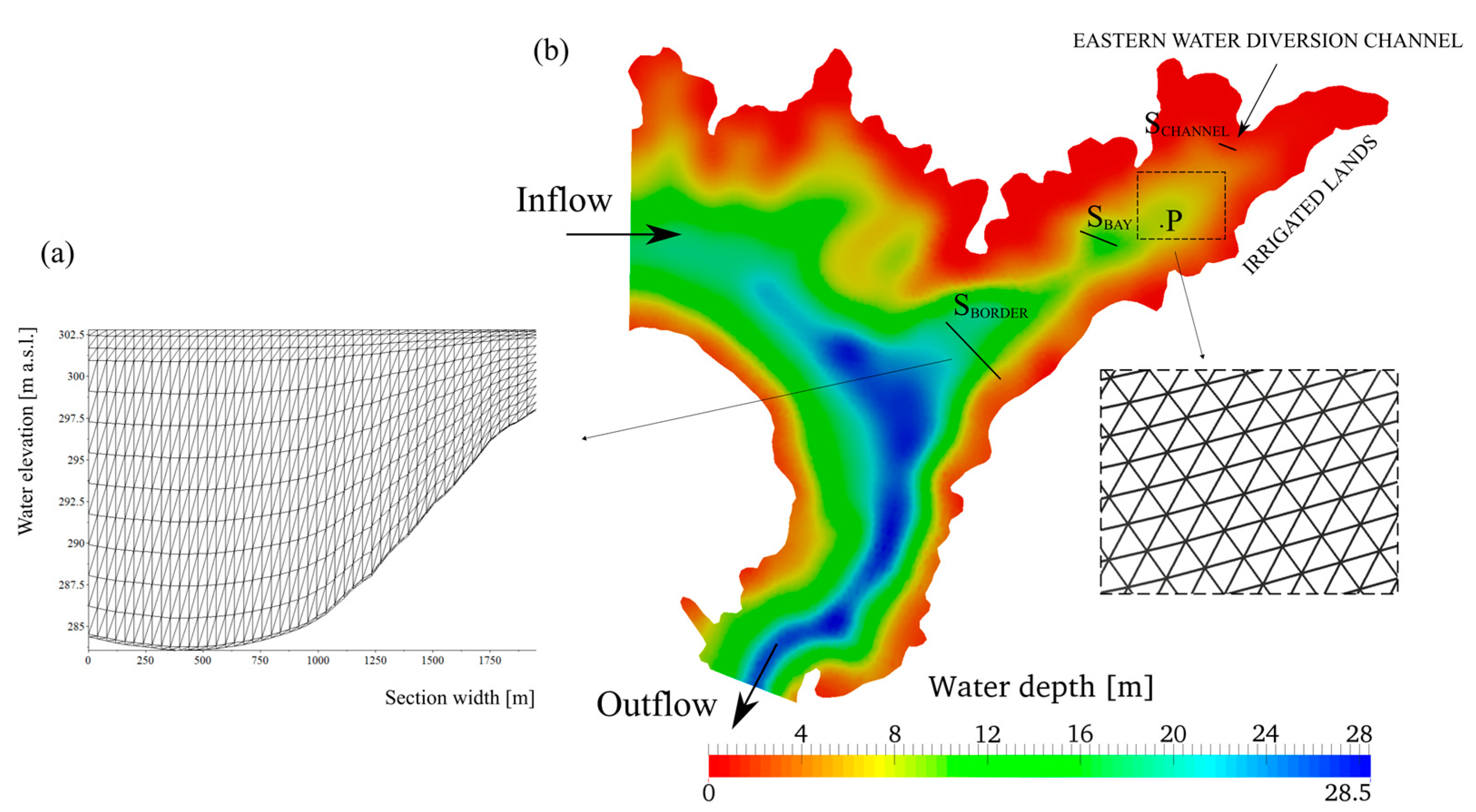
A three-dimensional (3D) model of Icó-Mandantes Bay was set up with the open TELEMAC-MASCARET modeling system, using the unstructured triangular grid created in reference [26] with the software Janet (Smile Consult GmbH). The domain covers the whole bay and part of the Itaparica Reservoir, the so-called main stream, in order to allow the water exchange between the two water bodies, as well as a realistic inflow and outflow to the system (Figure 2). The 3D grid consists of 14 layers. The resulting mesh consists of 13 prisms with variable height, depending on water depth [m]. The layers are equidistant in the whole vertical direction (10% of ), except for the refinements near the bottom (1% of ) and near the surface (2% and 6% of ), for capturing the effects of the correspondent friction stresses in higher detail. The final unstructured grid counts in total 162,932 nodes and 295,958 triangular elements, which are variable in length (range of 50 to 200 m). The surface area of the computational domain is around 128 km2, while the maximum lengths of the domain in x- and y-direction are respectively around 18 km and 16 km.
The simulations were conducted with a time step of 30 s for each case investigated, through parallel computing on the HLRN system (North German Association for the Promotion of High and Maximum Performance Calculation) [41], using 24 processors. This enabled the simulations to be very fast—e.g., running the wind-induced flow scenarios for 10 days took between 2 and 5 min.
4.2. Wind and Temperature Data
Meteorological data is available since year 2002 on the database SINDA [42], a Brazilian integrated system of environmental data. Data of wind and temperature were recorded every three hours at the nearest weather station available located in Floresta (PE), a municipality about 25–30 km distant from the Icó-Mandantes Bay.
Wind data has been statistically analyzed in previous work [25]. The magnitude range of the entire sample comprises values between 0 and 15 m/s, with maximum 10% of values between 15 and 20 m/s. The predominant wind direction is 140° (from SE to NW) and the mean speed is 5.5 m/s, according to the normal Gauss distribution.
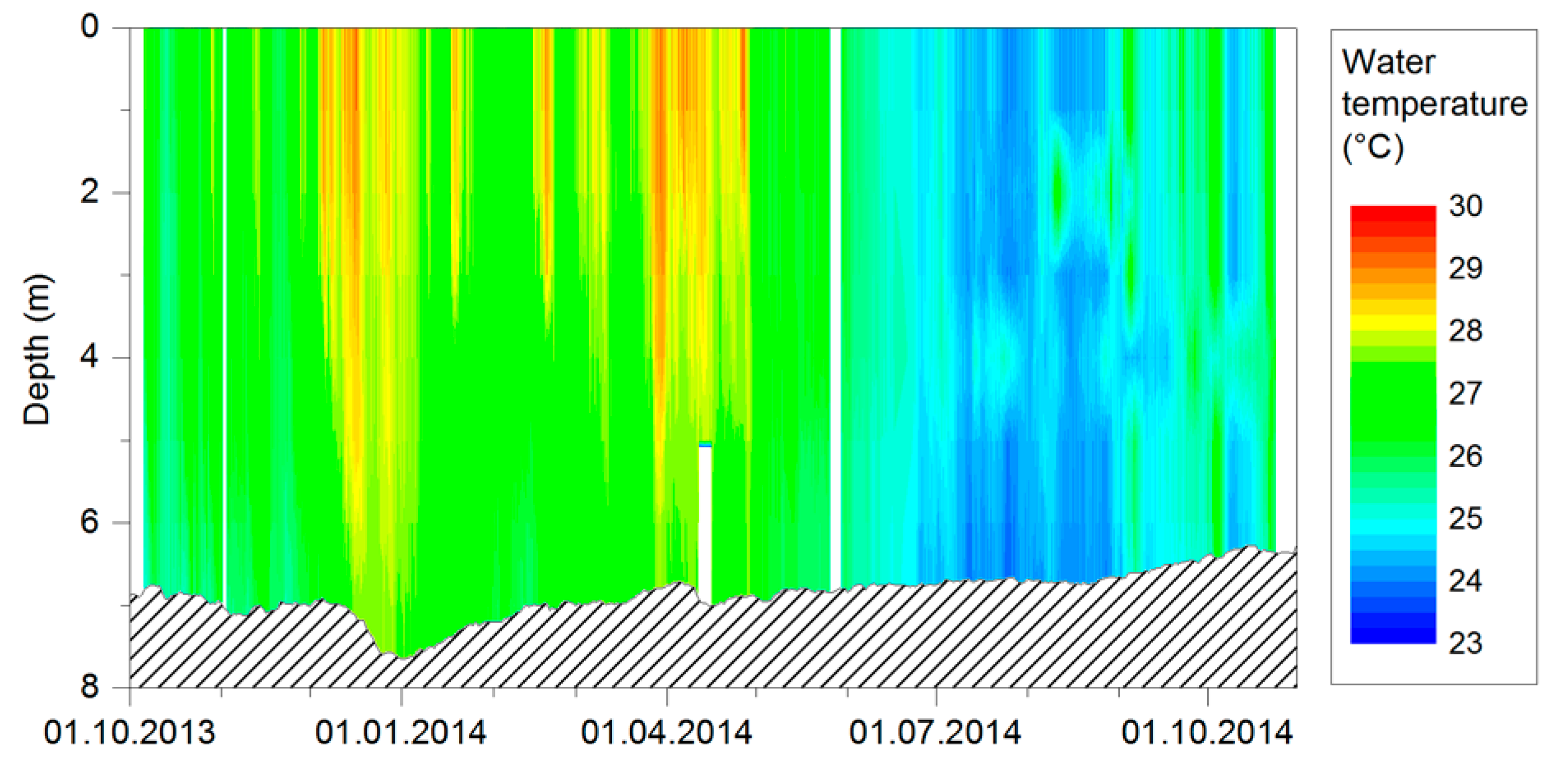
Air temperature was also recorded between 2002 and 2016. The annual average is ~26 °C [5], with a high daily variability (ΔT) of about 10 to 20 °C/d, characterized by increasing values over the day (9 a.m.–6 p.m.) up to a maximum of 38–40 °C and decreasing over the night (6 p.m.–9 a.m.) until a minimum of 17–22 °C. Regarding water temperatures, Selge et al. [37] reported mean values of 24.8 °C for dry and 27.7 °C for rainy periods. During the rainy periods, water temperatures increase and do not allow a stable thermal stratification, due to night cooling and convective currents, known as atelomixis [43,44]. This partial mixing down to the hypolimnion occurs with a frequency of every few days. Dry periods are characterized by stronger winds, higher cloud cover and high evaporation rates, resulting in lower water temperature and no stable thermal stratification, too. In order to have an idea of the stratification in the inner bay, we reported in Figure 3 the water temperatures over the depth for the period between October 2013 and October 2014 [39].
4.3. Simulation Scenarios
The scenarios presented in this article are:
- REF (reference): application of constant mean wind on normal reservoir-operating conditions;
- WIND: simulation of a windstorm event, i.e., imposing 6 h of extreme wind, starting from REF;
- HEAT: simplified approach to simulate the effects of water heating, applying a constant temperature change (ΔT) between water and air equal to 10 °C, starting from REF;
The same boundary conditions concerning the flow were set up for the three scenarios (REF, WIND and HEAT). In detail, a constant water discharge of 2060 m3/s (mean value for the Itaparica Reservoir under normal operating conditions) was assumed at the inflow boundary, while at the outflow boundary a constant water level of 302.8 m a.s.l. (mean value at the Luiz Gonzaga dam [35]). The remaining lateral boundaries were set as closed walls with slip condition (i.e., the tangential velocity is different from zero).
The reference case REF was simulated until steady state was reached, considering the action of mean wind velocity and direction (i.e., 5.5 m/s, 140°). This scenario served as initial conditions, as well as a basis for comparison for the other scenarios (WIND and HEAT).
The WIND case represents a windstorm event, occurring for some hours during 1 day, disturbing the equilibrium conditions of REF. The extreme wind of 20 m/s (representing a gale, according to the Beaufort scale [45]) was applied for 6 h between 9 a.m. and 3 p.m., the usual times of the day at which wind increases, within a total duration of simulation of 1 day (Table 1). Afterwards, the computation was continued for 5 days in order to estimate the time needed by the system to return to equilibrium. The direction of the wind (140°) was kept constant to isolate the effects of the wind’s magnitude. For this scenario, the focus is exclusively on the hydrodynamics, i.e., on the wind-induced circulation patterns (horizontal and vertical) and on the local eddies caused by the wind’s variation.
The HEAT case includes the transport of an active tracer; in particular, a constant temperature difference (ΔT) of 10 °C between water and air, respectively 26.5 °C and 36.5 °C, was imposed to the system. A Dirichlet type condition for the water temperature at the inflow equal to 26.5 °C for HEAT and a Neumann type at the outflow were additionally prescribed for the tracer, imposing a zero gradient of temperature. The surface boundary condition, regulating the heating of the water surface, is reported and explained in Equations (5) and (6) of Section 2. This was chosen as a first approach, in order to verify whether heating the water surface by the atmosphere would affect the 3D flow field. If this is not the case (thus, the impact is minor), the simulation of a temperature’s daily cycle would induce even lower changes.
4.4. Observation Points and Sections
First, mass conservation was checked through the output of the initial and final water masses (volumes [m3]), as well as the outflowing discharges at the correspondent boundaries at each time step. The 3D results were further analyzed over each horizontal layer and over time. In order to simplify the analysis, but still fully representing the results, the layers were chosen at the bottom (LBOTTOM), at an intermediate level (LINTERMEDIATE) and near the surface (LTOP) (Figure 4). Afterwards, different vertical cross-sections have been chosen in some selected areas of the computational domain: SBORDER at the border between the two different behaving systems (bay and reservoir main stream); SBAY in the center of the bay and SCHANNEL next to the intake of the water diversion channel (Figure 2b). In Figure 2a, it is possible to observe the refinement of the mesh at the top and at the bottom for section SBORDER.
5. Results
5.1. Reference Case (REF)
The REF scenario is the reference case and represents the initial conditions for WIND and HEAT. Results show that the main stream is characterized by deeper waters (up to a maximum water depth of 30 m) while the bay is off-stream, with a maximum depth of ~20 m and large shallow areas along the shores lower than 3 m depth. The water in the bay is almost stagnant and the flow is mainly induced by the SE wind.
The REF results over the horizontal layers are shown in Figure 4. Looking at the variations along the water depth, it was possible to notice that the superficial levels are generally wind-oriented, while upwind (against the wind) the deeper ones (near the bed). We encountered the so-called wind-induced return flows: wind aligns with the flow at the surface, imposing return flow areas along the bottom [33]. Some eddies were detected near the bottom, also observable in the intermediate layers, but with higher frequency and horizontally dislocated.
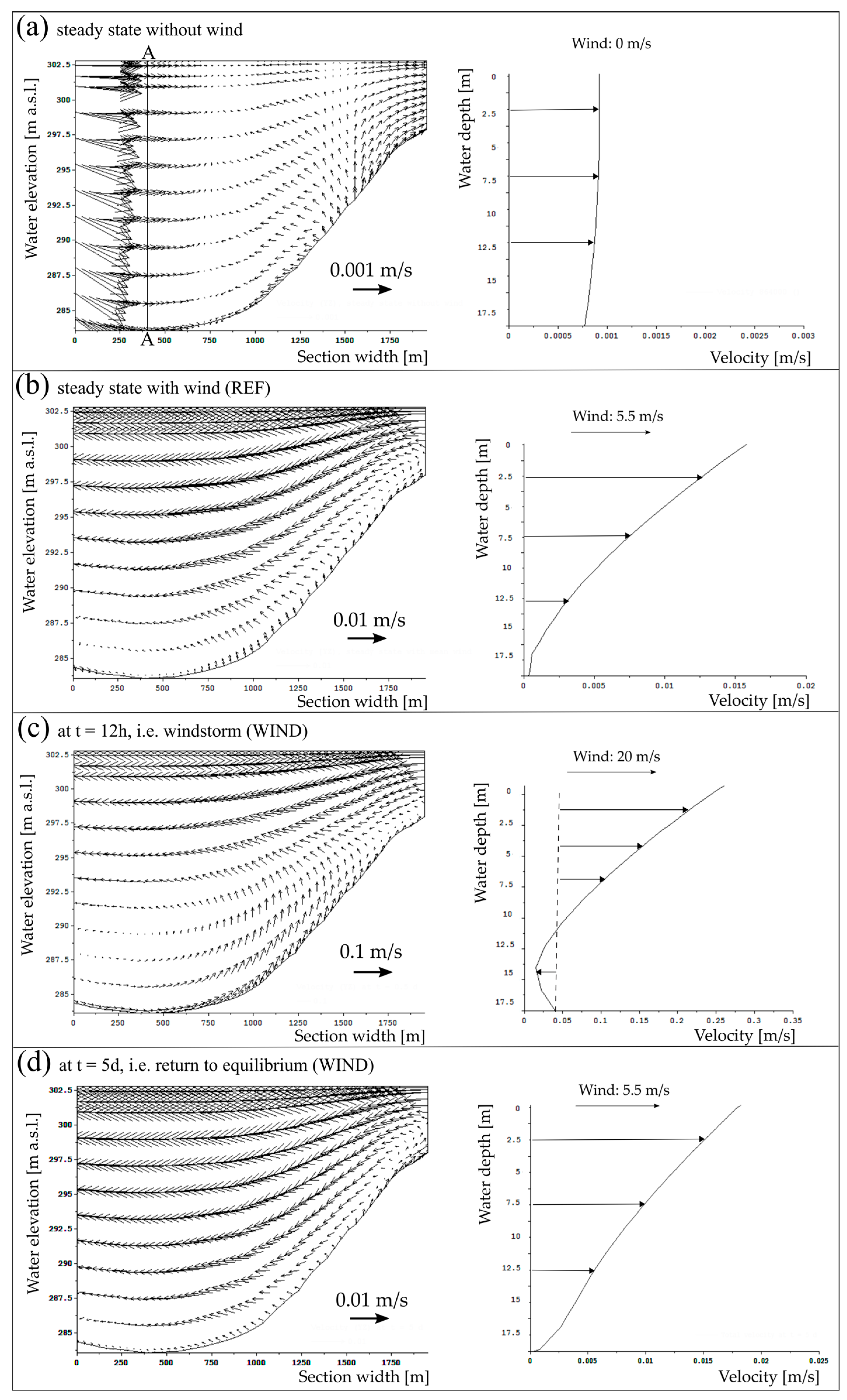
The simulations were also conducted in absence of wind, in order to better observe the changes. When the wind was neglected, the vertical profiles of velocity resulted to be parabolic in the reservoir main stream part, characterized by maximum values near the surface, while in the bay quite linear with constant values very close to zero over the entire water column (stagnation areas). Otherwise, when the mean wind was considered (i.e., REF), the velocities decreased or increased in the superficial layers, respectively if the flow was upwind or in wind direction. For instance, in section SBORDER shown in Figure 2, the vertical magnitude of velocity (w) was comparable with the horizontal ones (u, v)—therefore we incurred some 3D effects (Figure 5b).
5.2. Windstorm Scenario (WIND) and Return to Equilibrium Condition
The results of this scenario were compared before, during and after the windstorm (20 m/s, 140°). The changes concerning the horizontal output of the flow field, as well as the variations over the vertical direction, can be observed in Figure 4b. The magnitude and the orientation of velocities were significantly influenced by the wind, but to different extents. The range of velocities increased at least of one order of magnitude during the windstorm: up to 10−1 m/s in the reservoir main stream and up to 10−2 m/s in the bay part.
During the storm—i.e., at 12 h (Figure 4b)—the flow field is overall wind-oriented on the superficial layers, except for the main stream region, where a big horizontal clockwise circulation of approx. 2-km2-area was formed. This horizontal pattern was still observable on the deeper intermediate and bottom layers, but rather shifted downstream, accompanied by an additional anticlockwise circulation of similar dimensions closer to the northern shore. On LBOTTOM and LINTERMEDIATE in the bay, the flow field is weaker and more chaotic, compared to LTOP. In areas where < 3 m, the velocities are often wind-oriented over the entire water depth. Observing the results later on at 24 h, the number of eddies increase in general over the superficial and intermediate layers, characterized by eddies of ~500 m to 1 km in diameter. This seems to be due to a sort of relaxation and readjustment of the flow field, attempting to return to initial equilibrium conditions. Velocities on LBOTTOM are very close to zero. The variable and more irregular flow at this time step suggest the presence of 3D circulation.
Looking at various cross-sections in the domain, different flow behaviors were observed. Along the reservoir main stream, where water is deeper, the velocity profiles have a parabolic shape, which is typical for open channels. There, the influence of the wind is evident through a deformation of the curve closer to the surface; the wind slows down the velocities near the surface, in the case of upwind flow, invoking the occurrence of return flows. Specifically, in section SBORDER (Figure 2 and Figure 5), located at the imaginary border between the bay and the main stream, where mutual exchange processes take place, we observe water moving from the shores to the deeper inner parts (surface layers) and a weak upwelling for REF (Figure 5b), which becomes wider involving bigger part of the water depth during the windstorm, accompanied by a velocity’s increase at least of one order of magnitude (at t = 12 h, Figure 5c). In that region, the horizontal and vertical flow components are in a similar range.
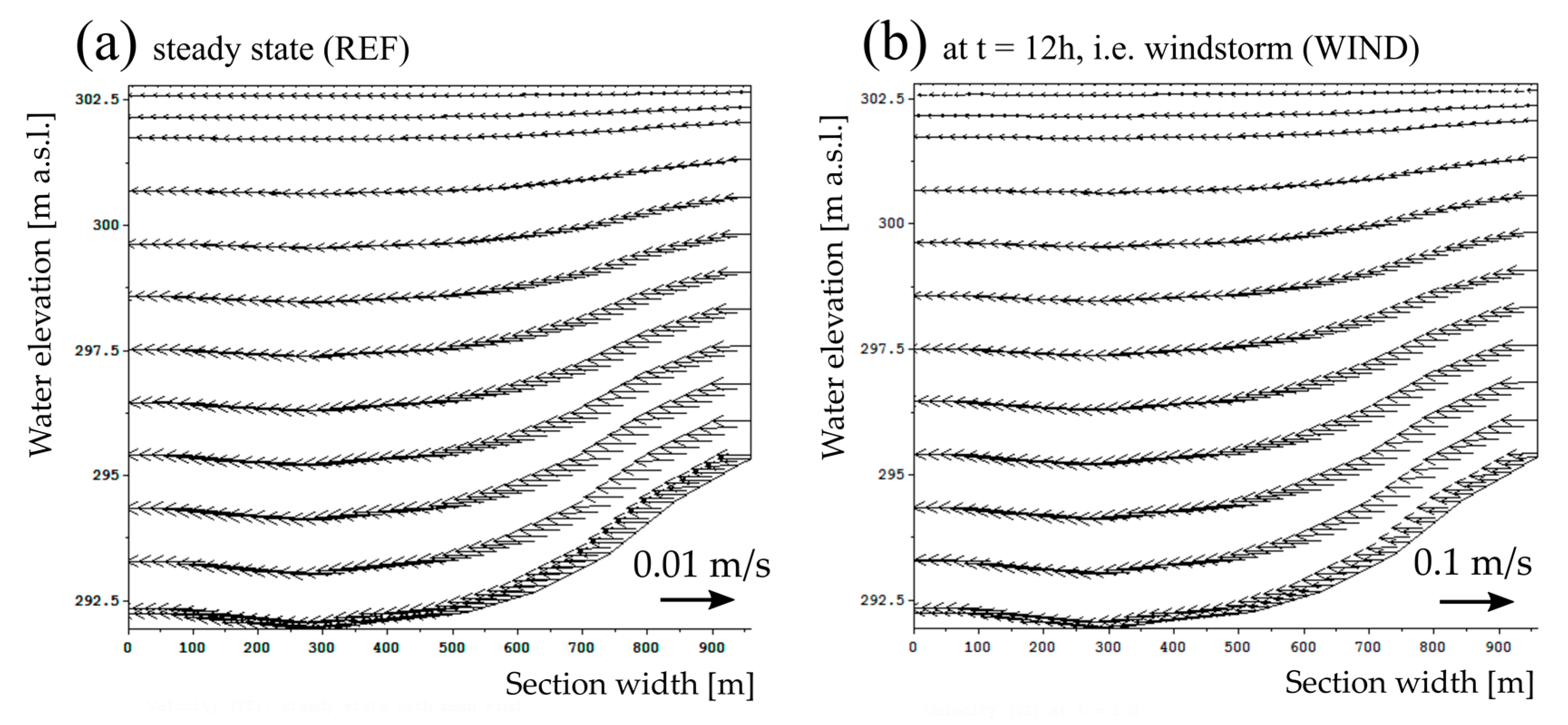
Additionally, the behavior of the flow field in the center of the bay (namely SBAY of Figure 2) is shown in Figure 6. Comparing REF and WIND (the latter during the windstorm, i.e., at 12 h): the flow velocities are mostly wind-oriented in both cases in the vertical direction, with an increase of velocities of one order of magnitude for the latter (scale of 0.1 m/s). This flow pattern was maintained over time; therefore, the further steps are not reported. Finally, the WIND scenario was compared to REF also in the cross-section at the intake of the water diversion channel (namely SCHANNEL of Figure 2) and shown in Figure 7. In REF, the water velocities were ≤ 0.005 m/s, while during strong wind they increased by more than one order of magnitude (higher near to the bed), but they kept the same direction over the water depth. After around three days of simulation, the flow configuration became similar to pre-disturbance conditions, i.e., REF. In other shallow areas of the bay along the shores near the irrigated lands, the flow was mostly wind-oriented over the entire depth, both for REF and for WIND, because of the intensity of the wind, inducing movement in those shallow and stagnant waters.
Since steady state was not reached yet one day after the windstorm, the computation was continued for five additional days, under the same conditions as REF i.e., constant mean flow and mean wind. The changes observed at the end of this computation were lower than 1 × 10⁻³ m/s, concerning mean velocities. Since the discharges at the outflow boundary reached the steady state already after four days, with differences <0.1 m3/s, and changes in the cross-sections and over the layers were no longer substantial, we can affirm that the flow field returned to equilibrium by that time. The water mass volumes V [m3] were always conserved after each time step (ΔV lower than 0.01%).
5.3. Surface Water Heating Scenario (HEAT)
The results were analyzed at different time steps (i.e., after few hours and until one month), in order to identify the time needed by the entire system to shift to a new equilibrium under the imposed constant conditions (Section 4.3).
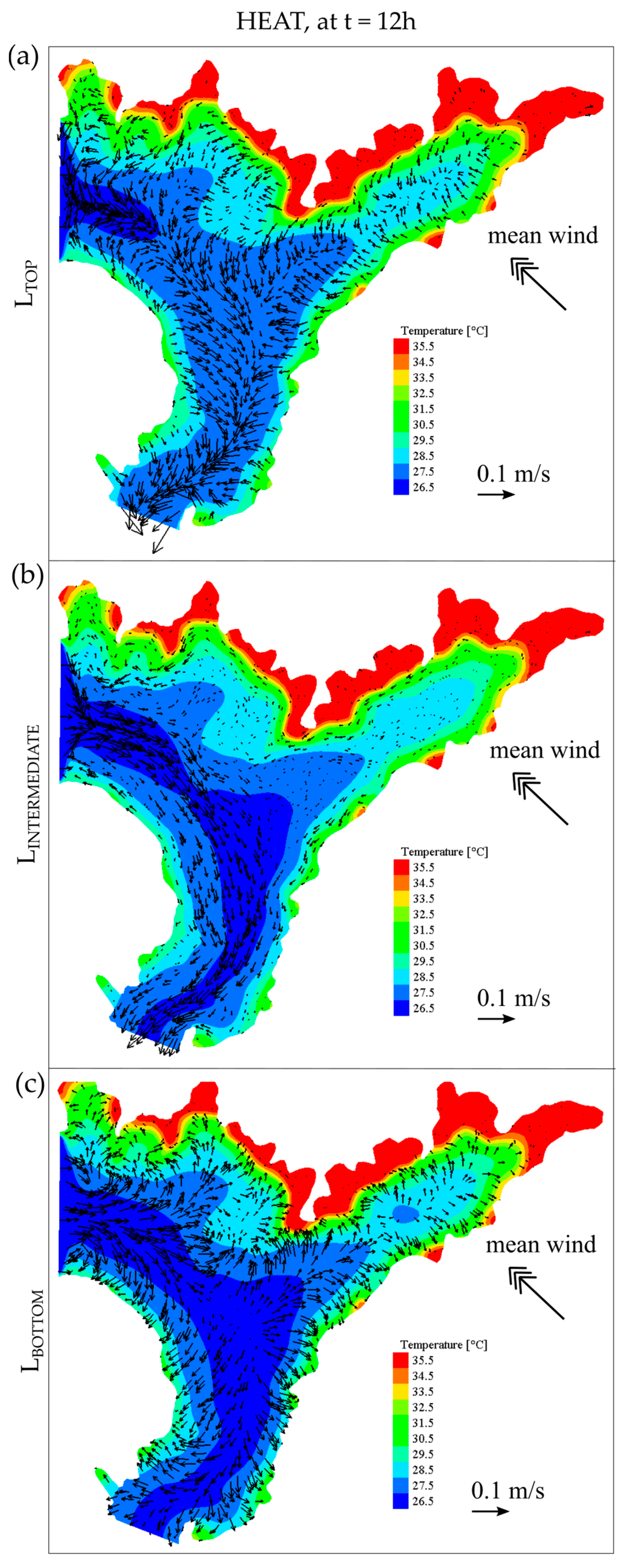
Looking at LBOTTOM, already during the first three hours up to one day, the heating effects induced the velocity vectors to be oriented from the deeper areas in direction of the shores (Figure 8c). The flow velocities were higher near the inflow (shown in Figure 2), along the main stream nearer to the western shore and in the bay as well. The opposite behavior was noticed in the superficial layers: the flow field oriented from the shallower (and warmer) peripheral parts to the deeper (colder) ones (Figure 8a). As expected for smaller water depths, the shores were heated faster. The weakest velocities occurred at the intermediate levels, and, close to LINTERMEDIATE, it was possible to observe a change in the flow configuration (bed- or surface-type). Figure 8 shows the outline of the temperatures and the flow field over the layers LBOTTOM, LINTERMEDIATE and LTOP after one day of simulation.
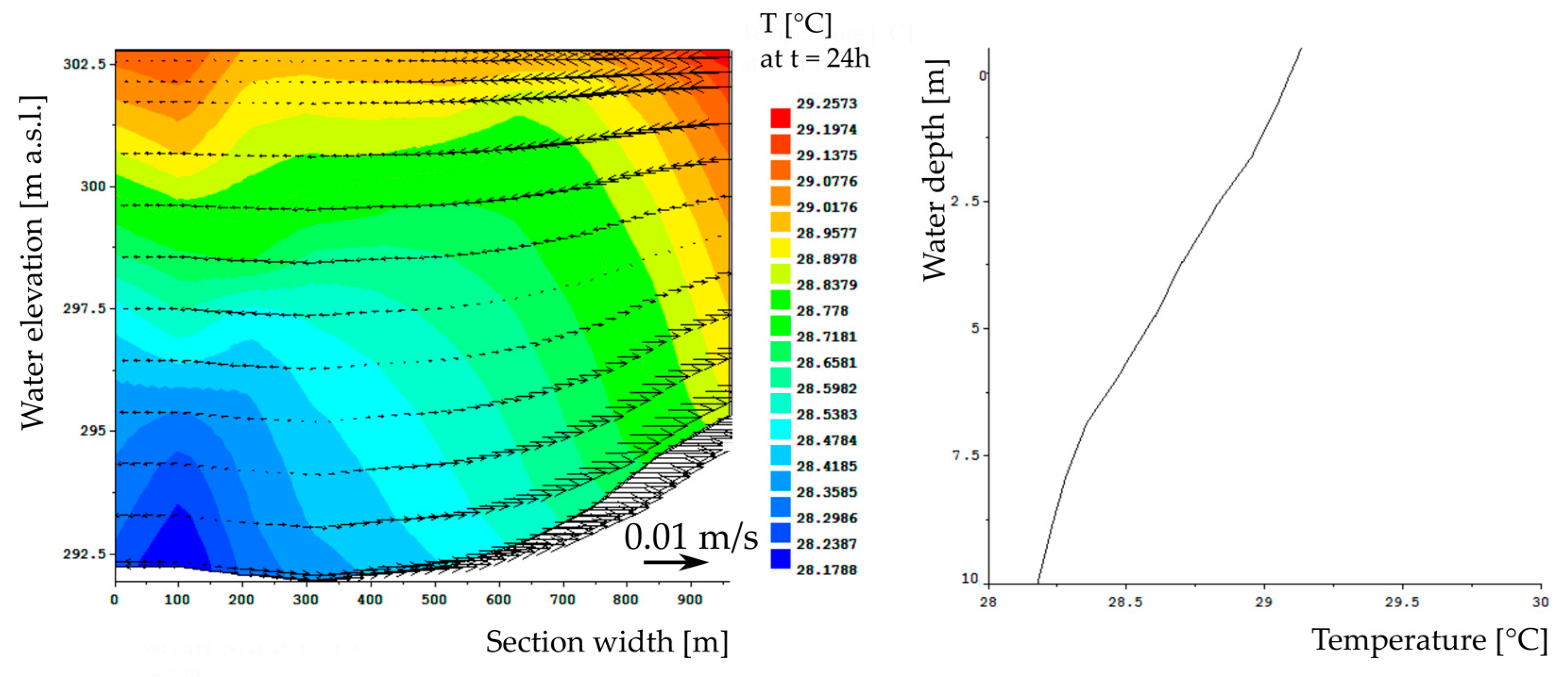
Continuing the calculations over one week, the velocities increased progressively in the entire domain: the flow configuration became rather stable after one day near the bottom, while in the upper layers (from LINTERMEDIATE to LTOP) was still affected by slight changes. After one week, the water mass in the entire bay reached temperatures higher than 30 °C, and, after 2 weeks, no changes were observable in the flow field (neither circulation nor values).
Figure 9 reports the outline of the total velocities in SBORDER (same of Figure 2 and Figure 5). Comparing Figure 4a and Figure 8, as well as Figure 5b and Figure 9, the flow field changed for HEAT and the velocity vectors are oriented in opposite directions at the surface relative to closer to the bottom, suggesting an anticlockwise movement of the water mass from the warmer to the colder areas. The velocities’ order of magnitude was in the same range as they were for the reference case REF (approx. 10−3 to 10−2 m/s), even if in the shallower part of the section the maximum values were at least doubled and the minimum were found in the central part of the section (approx. from 2 to 8 × 10⁻³ m/s). A slight progressive increase of the flow field was registered until one week, while the vertical configuration remained constant in time. Between one week and two weeks, the maximum velocities raised still of approx. 3 × 10⁻³ m/s and finally less than 1 mm/s between two weeks and one month. Looking at the temperature values in SBORDER, the minimum and maximum values were respectively 26.8 and 28.4 °C after 12 h, 27.5 and 29.5 °C after one day (Figure 9), 29.3 and 31.9 °C after three days, 30.6 and 33.5 after one week, 31.0 and 33.8 after one month. The maximum ΔT in water equal to maximum 2.5 to 3 °C reached after 3 days remained rather constant in time, while the overall values of temperature increased gradually until one week of simulation. Nevertheless, this did not occur over the vertical direction; thus, no stable stratification was observed. Additionally, the temperature gradient was formed between the shallow littoral areas and the center of the bay (Figure 9). In this case, the convective propagation of dense water intrusion occur after crossing temperature of maximum density, according to Boehrer and Schultze [12]. Afterwards, continuing the computation up to one month, no more changes were observed in the entire computational domain.
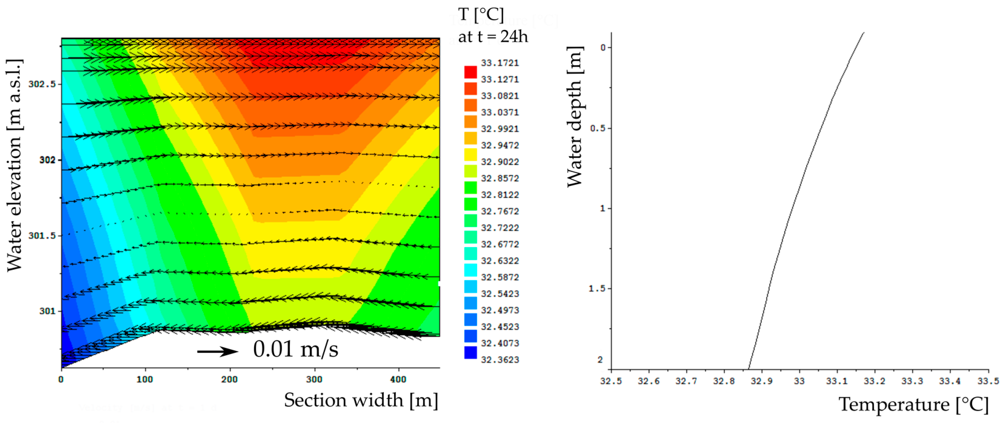
In the center of the bay, the flow velocities had similar order of magnitudes compared to SBORDER, even if with lower extremes. The temperatures had similar circulation patterns, but with higher vertical temperature gradient in SBAY (i.e., ≤1 °C, Figure 10). For the section next to the water diversion channel, the velocities were approximately doubled compared to SBORDER and there was an impact on the currents as well. The temperature difference observed over the water depth was even smaller (<0.5 °C, Figure 11).
5.4. Synthesis and Discussion
The results of the WIND and the HEAT scenarios, compared with the reference REF, showed that strong wind and density changes had an impact on the flow field, confirming a wide range of previous studies (e.g., [6,12,13,15,19]). On the one hand, while the configuration of the flow following the SE wind was maintained over time both horizontally and vertically, the imposed constant ΔT equal to 10 °C changed it substantially (e.g., the flow in the surface layers was induced from the shallow to the deeper waters). On the other hand, the wind had a much higher impact on the velocities—up to more than one order of magnitude. This is in agreement with De Marchis et al. [15] and Fenocchi et al. [13], who as well observed an increase of flow velocities of one order of magnitude in the case of wind and especially during storm events. For the density-induced flow, a velocity increase took place to a lower extend in some specific zones, e.g., on the bottom and superficial layers next to the lateral boundaries, while there was a general decrease at the intermediate water depths. According to Abbasi et al. [19], higher wind leads to higher return flows and shallow parts respond faster to air heating; the occurrence of these two phenomena are observable in our results, respectively in Figure 5c, Figure 8 and Figure 9. Moreover, during the heating phase, temperatures increase especially in the top layers near the water surface [19], as noticed as well in Figure 10 and Figure 11.
The vertical (w) and horizontal (u, v) components of velocities, as well as the water depths, were analyzed in detail for the cases investigated. The formers differed by at least two to three orders of magnitude (being u, v higher than w), except during the windstorm, when they reached a comparable range of values. The variation of the water depths has been analyzed at several observation points in the computational domain. They decreased in a range of 20 to 60 mm, comparing WIND to REF, due to the higher velocities, and increased in a range of 1 to 5 mm, comparing HEAT to REF, due to thermal expansion. Additionally, concerning the average values computed for the bay area, the water depths decreased by 7 mm, comparing WIND to REF, while they increased by 4 mm, comparing HEAT to REF. Thus, the variations of the water depths were considered absolutely minor (mm against means of at least 10 m).
Further summarizing the results, it can be mentioned that the flow field was able to return to equilibrium at least three days after a specific event (e.g., windstorm), as long as the disturbance (e.g., the wind) disappeared. Otherwise, it evolved until the achievement of a new steady state: few weeks were needed for the HEAT case.
Finally, a clear stable temperature stratification was not observable and the water column was well mixed over the entire computational time (up to one month). The ΔT in water over the vertical was generally lower than 0.5 °C (e.g., Figure 7), except for the most stagnant parts (e.g., Figure 10), where ΔT reached maximum 1 °C. Therefore, the water body is not classifiable as stratified (e.g., ΔT > 1 °C is one of the different criteria for stratification presented in [46]). This was considered a reasonable response of the system, in accordance with existing theories and limnological findings [5,12,39,44], due to the following reasons:
- the modeling showed that the 3D flow field was sensitive to the heating of water surface, inducing a vertical movement of the water mass and, thus, contributing to the vertical water mixing;
- the deeper reservoir main stream is characterized by a strong inflowing discharge from the upstream Sobradinho (here, approx. 2000 m3/s), which did not allow a stable stratification in the flow field concerning that part;
- according to Boehrer and Schultze [12], stratification can be established in the warm season if the lake is sufficiently deep (which is not the case here). Additionally, lakes are found to behave like an epilimnion (to be well mixed), in response to strong temperature gradients between water and air (10 °C in this case).
In conclusion, the applicability and reliability of the presented model is retained acceptable, certainly with some constraints. This is mainly due to the extreme complexity of the processes studied, the lack of measurements of some parameters or their availability in only one point of the domain [19,47].
5.5. Recommendations for Water Management
Small inland water bodies are often neglected in hydrological and water resources management plans, principally because it is difficult and expensive to monitor them [18,47]. Nevertheless, they are of greatest importance for the regional economic development and for the maintenance of water quality standards. The implications between the important hydrodynamic findings of the numerical modeling for water management at the local scale are rarely explored, but need to be outlined. Currently, the water diversion channel is not yet in operation, while the withdrawals for irrigation agriculture are under the responsibility of CODEVASF (Development Company of the São Francisco and Parnaíba Valleys), outsourcing the engineering company PLENA Engenharia. The users are allowed to pump water for a few hours per day (usually 8–12 h), with a maximum (hourly) withdrawal between 1.4 and 1.7 m3/s [48,49,50,51].
In this work, we observed that the 3D effects on the flow field should be taken into account when managing the multiple water uses of the bay (addressed for instance in Arruda [49] and by the Ministry of National Integration [52]) deriving the following management suggestions and ideas for further investigations:
- The reservoir management needs a new approach, which requires first of all a differentiated analysis and evaluation for the reservoir main stream and its bays, characterized by different regimes (e.g., velocities), and where the 3D modeling is adopted as supporting tool;
- In particular, the withdrawals for drinking water and for irrigation agriculture, located in the tip of the bay and along the south-eastern shallow shores of the bay, should stop working during windstorms and at least three days afterwards, especially in case of rain after long droughts. In such event, two important facts would occur: (1) the mostly frequent wind from SE to NW induces the flow in a strong circulation current along the southeastern shore, where the irrigation lands are located, towards the tip of the bay; (2) the irrigation drainage systems would be overflowed and rich of nutrients and pollutants from the field, in case of rain, especially after long droughts. This implies that material such as suspended sediments, nutrients and rubbish would be transported towards the tip of the bay, where the water diversion is located. To be able to prevent or at least reduce such issues, it is important as well to launch initiatives among the rural communities such as the cleaning up of the shores areas from undesired material and the implementation of waste-collection procedures, since there is no proper disposal of waste or emissions by various consumptions in the region;
- Water surface heating due to strong temperature gradients would induce the suspended material present in the surface layers to be transported to the center of the bay, where the water is more stagnant even during a windstorm. On the contrary, the substances, nutrients and sediments deposited in the bottom layers would be conducted towards the shores and to the upper layers, with the occurrence of upwelling near land. This may increase phenomena like the accumulation of sediments in the shallow areas, which desiccate during the water level decrease due to hydropower operations, increasing the development of HAB. Further assessments using a water quality module are needed to support water management in this direction;
- The 3D model can then be used to identify high risk contamination areas in the Icó-Mandantes Bay, in order to plan promptly the necessary monitoring operations to ensure good standards of water quality for drinking water, as well as to control and regulate the development of further net cage aquaculture systems, in particular in the stagnant areas of the bay, next to the water intakes (water supply, irrigation).
6. Conclusions
To study the dynamics of surface water bodies such as lakes and reservoirs, the use of three-dimensional (3D) models is often preferred, since external forces as wind play an important role, enhancing 3D effects in the flow field and being one of the main drivers of water movement. This occurs in particular in more isolated peripheral bays, where the velocities are usually very low and characterized by different hydraulic regimes compared to the reservoir main streams. The case of the Icó-Mandantes Bay, one of the major branches of the Itaparica Reservoir (Sub-Middle São Francisco River, NE Brazil) was presented in the article and a 3D model was set up using the open TELEMAC-MASCARET modeling system [28]. The impacts of wind and heating of the water surface on the hydraulics of the bay have been meticulously explored, in the horizontal and vertical direction, detecting the consequent 3D effects. In conclusion, an advanced reservoir management for multiple uses has to consider also the issue of water quality and, for this case study, to focus especially on the need to keep oligotrophic levels, because the Icó-Mandantes Bay is already overcharged [39]. Since the hydrodynamics of such a water body are highly linked with water quality complex processes ([21]; e.g., algae growth and sediment fluxes), in future work, the existent 3D model should be coupled with a water quality module (e.g., with TELEMAC’s latest version 7.2 is currently feasible, using the WAQTEL module). In particular, further research should focus on (1) the risk of HAB development, mainly on their inoculation in the lentic bay areas and their interaction with the reservoir main stream, (2) the spreading of HAB and its impact on the withdrawals for drinking water or irrigation agriculture and (3) the adaptation of hydroelectric production to reduce water level fluctuations, in order to minimize the introduction of nutrients from the desiccated soils in the shallow areas and, thus, the greenhouse gases (GHG) emissions as well. Moreover, external forces such as the wind should be always included in the model, as well as the heating and cooling processes, since they have indeed complex and differentiated impacts of the hydraulics of water bodies such as the Icó-Mandantes Bay.
Acknowledgments
We gratefully acknowledge the German Federal Ministry of Education and Research (BMBF) for supporting this work, as part of the INNOVATE project. We would like to thank Tomaso Ferrando (Bristol University), Jonathan King (Cardiff University) and the anonymous reviewers for their precious comments. We acknowledge support by the German Research Foundation and the Open Access Publication Funds of Technische Universität Berlin.
Author Contributions
All authors contributed to the work presented in this paper. As specific contributions, Elena Matta and Reinhard Hinkelmann provided the concept and designed the article content; Elena Matta prepared, implemented the model and simulations and wrote the manuscript; Florian Selge and Günter Gunkel contributed in providing the data and observations, fieldwork, developing the data analysis; Günter Gunkel and Reinhard Hinkelmann also contributed proofreading the manuscript and verifying the results.
Conflicts of Interest
The authors declare no conflict of interest.
References
- Marengo, J.A.; Torres, R.R.; Alves, L.M. Drought in Northeast Brazil—Past, present, and future. Theor. Appl. Climatol. 2016, 1–12. [Google Scholar] [CrossRef]
- Siegmund-Schultze, M. (Ed.) Guidance Manual—A Compilation of Actor-Relevant Content Extracted from scientific Results of the INNOVATE Project; Universitätsverlag der TU Berlin: Berlin, Germany, 2017; Volume 128. [Google Scholar]
- Gunkel, G.; Sobral, M. Re-oligotrophication as a challenge for a tropical reservoir management with reference to Itaparica Reseroir, São Francisco, Brazil. Water Sci. Technol. 2013, 67, 708–714. [Google Scholar] [CrossRef] [PubMed]
- Coutinho, R.M.; Kraenkel, R.A.; Prado, P.I.; Scheffer, M.; Guttal, V.; Ives, A. Catastrophic Regime Shift in Water Reservoirs and São Paulo Water Supply Crisis. PLoS ONE 2015, 10, e0138278. [Google Scholar] [CrossRef] [PubMed]
- Gunkel, G.; Selge, F.; Keitel, J.; Lima, D.; Calado, S.; Sobral, M.; Rodriguez, M.; Matta, E.; Hinkelmann, R.; Casper, P.; et al. Management of a tropical reservoir (Itaparica, São Francisco, Brazil): Multiple water uses, impact, and ecological sustainability. Reg. Environ. Chang. 2017. submitted. [Google Scholar]
- Zamani, B.; Koch, M.; Hodges, B.R.; Fakheri-Fard, A. Pre-impoundment assessment of the limnological processes and eutrophication in a reservoir using three-dimensional modeling: Abolabbas reservoir, Iran. J. Appl. Water Eng. Res. 2016, 1–14. [Google Scholar] [CrossRef]
- Kennedy, R.H.; Thornton, K.W.; Ford, D.E. Characterization of the reservoir ecosystem. In Microbial Processes in Reservoirs; Gunnison, D.E., Ed.; Junk: Boston, MA, USA, 1985; pp. 27–38. [Google Scholar]
- Smith, V.H.; Tilman, G.D.; Nekola, J.C. Eutrophication: Impacts of excess nutrient inputs on freshwater, marine, and terres-trial ecosystems. Environ. Pollut. 1999, 100, 179–196. [Google Scholar] [CrossRef]
- Hattermann, F.F.; Koch, H.; Liersch, S.; Silva, A.L.; Azevedo, R.; Selge, F.; Silva, G.N.S.; Matta, E.; Hinkelmann, R.; Fischer, P.; et al. Climate and land use change impacts on the water-energy-food nexus in the semi-arid northeast of Brazil—Scenario analysis and adaptation options. Reg. Environ. Chang. 2017. submitted. [Google Scholar]
- Falconer, R.A.; George, D.G.; Hall, P. Three dimensional numerical modeling of wind-driven circulation in a shallow homogeneous lake. J. Hydrol. 1991, 124, 59–79. [Google Scholar] [CrossRef]
- Hattermann, F.F.; Weiland, M.; Huang, S.; Krysanova, V.; Kundzewicz, Z.W. Model-Supported Impact Assessment for the Water Sector in Central Germany Under Climate Change—A Case Study. Water Resour. Manag. 2011, 25, 3113–3134. [Google Scholar] [CrossRef]
- Boehrer, B.; Schultze, M. Stratification of lakes. Rev. Geophys. 2008, 46, 1–27. [Google Scholar] [CrossRef]
- Fenocchi, A.; Petaccia, G.; Sibilla, S. Modelling flows in shallow (fluvial) lakes with prevailing circulations in the horizontal plane: Limits of 2D compared to 3D models. J. Hydroinf. 2016, 18, 928–945. [Google Scholar] [CrossRef]
- De Marchis, M.; Ciraolo, G.; Nasello, C.; Napoli, E. Wind- and tide-induced currents in the Stagnone lagoon (Sicily). Environ. Fluid Mech. 2012, 12, 81–100. [Google Scholar] [CrossRef] [Green Version]
- De Marchis, M.; Freni, G.; Napoli, E. Three-dimensional numerical simulations on wind- and tide-induced currents: The case of Augusta Harbour (Italy). Comput. Geosci. 2014, 72, 65–75. [Google Scholar] [CrossRef] [Green Version]
- Napoli, E.; Armenio, V.; De Marchis, M. The effect of the slope of irregularly distributed roughness elements on turbulent wall-bounded flows. J. Fluid Mech. 2008, 613, 385–394. [Google Scholar] [CrossRef]
- Abeysinghe, K.G.A.M.C.S.; Nandalal, K.D.W.; Piyasiri, S. Prediction of thermal stratification of the Kotmale reservoir using a hydrodynamic model. J. Natl. Sci. Found. Sri Lanka 2005, 33, 25–36. [Google Scholar] [CrossRef]
- Liebe, J.R.; Andreini, M.; Giesen, N.; van de Steenhuis, T.S. The small reservoirs project: Research to improve water availability and economic development in rural semi-arid areas. In The Hydropolitics of Africa: A Contemporary Challenge; Kittisou, M., Ndulo, M., Nagel, M., Grieco, M., Eds.; Cambridge Scholars Publishing: Newcastle, UK, 2007. [Google Scholar]
- Abbasi, A.; Annor, F.; van de Giesen, N. Investigation of Temperature Dynamics in Small and Shallow Reservoirs, Case Study: Lake Binaba, Upper East Region of Ghana. Water 2016, 8, 84. [Google Scholar] [CrossRef]
- Ladwig, R.; Kirillin, G.; Hinkelmann, R.; Hupfer, M.; Ladwig, R.; Kirillin, G.; Hinkelmann, R.; Hupfer, M. Lake on life support: Evaluating urban lake management measures by using a coupled 1D-modelling approach. In EGU General Assembly 2017; Copernicus GmbH, Göttingen, Germany: Vienna, Austria, 2017. [Google Scholar]
- Ji, Z.-G. Hydrodynamics and Water Quality: Modeling Rivers, Lakes, and Estuaries; Wiley & Sons, Inc.: Hoboken, NJ, USA, 2008; ISBN 978-0-470-13543-3. [Google Scholar]
- Bednarz, T.P.; Lei, C.; Patterson, J.C. Unsteady natural convection induced by diurnal temperature changes in a reservoir with slowly varying bottom topography. Int. J. Therm. Sci. 2009, 48, 1932–1942. [Google Scholar] [CrossRef]
- Castro, C.N.D.C. Transposição Do Rio São Francisco: Análise De Oportunidade Do Projeto. Ipea. Gov. Br. 2011. Available online: http://repositorio.ipea.gov.br/handle/11058/3776 (accessed on 8 September 2017).
- Gunkel, G.; Matta, E.; Selge, F.; Silva, G.M.N.; da Sobral, M. Carrying capacity limits of net cage aquaculture in brazilian reservoirs. Rev. Bras. Ciênc. Ambient. 2015, 128–144. [Google Scholar] [CrossRef]
- Matta, E.; Özgen, I.; Cabral, J.; Candeias, A.L.; Hinkelmann, R. Simulation of Wind-induced Flow and Transport in a Brazilian bay. In International Conference on Hydroscience & Engineering (ICHE); Lehfeldt, R., Kopmann, R., Eds.; Bundesanstalt für Wasserbau: Hamburg, Germany, 2014; ISBN 978-3-939230-32-8. [Google Scholar]
- Matta, E.; Selge, F.; Gunkel, G.; Rossiter, K.; Jourieh, A.; Hinkelmann, R. Simulations of nutrient emissions from a net cage aquaculture system in a Brazilian bay. Water Sci. Technol. 2016, 73, 2430–2435. [Google Scholar] [CrossRef] [PubMed]
- Matta, E.; Koch, H.; Selge, F.; Simshäuser, M.N.; Rossiter, K.; Nogueira da Silva, G.M.; Gunkel, G.; Hinkelmann, R. Modeling the impacts of climate extremes and multiple water uses to support water management in the Icó-Mandantes Bay, Northeast Brazil. J. Water Clim. Chang. 2017. submitted. [Google Scholar]
- Hervouet, J.M. Hydrodynamics of Free Surface Flows. Modelling with the Finite Element Method; John Wiley & Sons: Hoboken, NJ, USA, 2007; ISBN 9780470035580. [Google Scholar]
- Özgen, I.; Seemann, S.; Candeias, A.L.; Koch, H.; Simons, F.; Hinkelmann, R. Simulation of hydraulic interaction between Icó-Mandantes bay and São Francisco river, Brazil. In Sustainable Management of Water and Land in Semiarid Areas; Editora Universitaria: Recife, Brazil, 2013; pp. 28–38. ISBN 9788541502597. [Google Scholar]
- Hutchinson, G.E. A Treatise on Limnology, Vol. 1. Geography, Physics and Chemistry; John Wiley: New York, NY, USA, 1957. [Google Scholar]
- Hinkelmann, R. Efficient Numerical Methods and Information-Processing Techniques in Environment Water; Inst. für Wasserbau: Stuttgart, Germany, 2003; ISBN 3933761204. [Google Scholar]
- Cirilo, J.A. Análise dos Processos Hidrológico—Hydrodinâmicos na Bacía Do Rio São Francisco. (Hydrological and Hydrodynamic Processes Analysis in São Francisco River Basin.). Ph.D. Thesis, UFPE, Recife, Brazil, 1991. [Google Scholar]
- Jourieh, A. Multi-Dimensional Numerical Simulation of Hydrodynamics and Transport Processes in Surface Water Systems in Berlin. Ph.D. Thesis, Technische Universität Berlin, Berlin, Germany, 2015. [Google Scholar]
- Sweers, H.E. A nomogram to estimate the heat-exchange coefficient at the air-water interface as a function of wind speed and temperature; a critical survey of some literature. J. Hydrol. 1976, 30, 375–401. [Google Scholar] [CrossRef]
- CHESF, Companhia Hidro Elétrica Do São Francisco. Sistemas de Geração: Luiz Gonzaga. Available online: https://www.chesf.gov.br/ (accessed on 11 January 2015).
- Keitel, J.; Zak, D.; Hupfer, M. Water level fluctuations in a tropical reservoir: The impact of sediment drying, aquatic macrophyte dieback, and oxygen availability on phosphorus mobilization. Environ. Sci. Pollut. Res. 2015. [Google Scholar] [CrossRef] [PubMed]
- Selge, F.; Matta, E.; Hinkelmann, R.; Gunkel, G. Nutrient load concept-reservoir vs. bay impacts: A case study from a semi-arid watershed. Water Sci. Technol. 2016, 74, 1671–1679. [Google Scholar] [CrossRef] [PubMed]
- Lima, D. The Role of Water Level Fluctuations in the Promotion of Phytoplankton and Macrophyte Pioneer Species in a Tropical Reservoir in the Brazilian Semiarid; TU Berlin: Berlin, Germany, 2017. [Google Scholar]
- Selge, F. Aquatic Ecosystem Functions and Oligotrophication Potential of the ITAPARICA Reservoir, São Francisco River, in the Semi-Arid Northeast Brazil; ITU Schriftenreihe Nr. 33; Papierflieger Verlag Clausthal-Zellerfeld: Clausthal-Zellerfeld, Germany, 2017; ISBN 978-3-86948-580-5. [Google Scholar]
- Lopes, F.B.; Andrade, E.M.; de Meireles, A.C.M.; Becker, H.; Batista, A.A. Assessment of the water quality in a large reservoir in semiarid region of Brazil. Rev. Bras. Eng. Agrícola Ambient. 2014, 18, 437–445. [Google Scholar] [CrossRef]
- HLRN (Norddeutsche Verbund für Hoch- und HöchstLeisTungsRechNen). Available online: https://www.hlrn.de/home/view/Main/WebHome (accessed on 8 August 2017).
- INPE Sistema Integrado de Dados Ambientais. Available online: http://www.sinda.crn2.inpe.br/PCD/SITE/novo/site/index.php (accessed on 8 August 2017).
- Gunkel, G.; Casallas, J. Limnology of an equatorial high mountain lake—Lago San Pablo, Ecuador: The significance of deep diurnal mixing for lake productivity. Limnologica 2002, 32, 33–43. [Google Scholar] [CrossRef]
- Selge, F.; Gunkel, G. Water Reservoirs: Worldwide distribution , morphometic characteristics and thermal stratification processes. In Sustainable Management of Water and Land in Semiarid Areas; Universidade Federal de Pernambuco (UFPE): Recife, Brazil, 2013; ISBN 9788541502597. [Google Scholar]
- Beaufort Wind Force Scale—Met Office. Available online: http://www.metoffice.gov.uk/guide/weather/marine/beaufort-scale (accessed on 8 August 2017).
- Engelhardt, C.; Kirillin, G. Criteria for the onset and breakup of summer lake stratification based on routine temperature measurements. Fundam. Appl. Limnol. Arch. Hydrobiol. 2014, 184, 183–194. [Google Scholar] [CrossRef]
- Abbasi, A. Energy Balance and Heat Storage of Small Shallow Water Bodies in Semi-Arid Areas; TU Delft: Delft, The Nederlands, 2016. [Google Scholar]
- Ministério da Integração National (Ministry of National Integration) Projeto de Integração do Rio São Francisco (Project of Integration of the São Francisco River). Available online: http://www.integracao.gov.br/web/projeto-sao-francisco/entenda-os-detalhes (accessed on 9 August 2017).
- De Arruda, N.O. Controle do Aporte de Fósforo no Reservatório de Itaparica Localizado no Semiárido Nordestino. Ph.D. Thesis, Federal University of Pernambuco (UFPE), Recife, Brazil, 2015. [Google Scholar]
- Projetos Públicos de Irrigação—Companhia de Desenvolvimento dos Vales do São Francisco e do Parnaíba, CODEVASF (Public Irrigation Projects—Development Company of the São Francisco and Parnaíba Valleys, CODEVASF). Available online: http://www.codevasf.gov.br/principal/perimetros-irrigados (accessed on 26 September 2017).
- National Water Agency (ANA). Resolution 411 of the 22 September 2005, Brasilia, Brazil. Available online: http://www.integracao.gov.br/web/projeto-sao-francisco/documentos-tecnicos (accessed on 9 October 2017).
- Ministério da Integraçao National (Ministry of National Integration). Relatorio de Integração do Rio São Francisco com Bacias Hidrograficas do Nordeste Setentrional (Report of the Integration of the São Francisco River with Hydrographical Basins of the Northeast). 2004. Available online: http://www.integracao.gov.br/web/projeto-sao-francisco/documentos-tecnicos (accessed on 9 October 2017).
Figure 1.
Location of the study area: Northeast Brazil (a), and capture of Itaparica Reservoir and Icó-Mandantes Bay (b). Adapted by the author from Google Earth (2016) and Lopes et al. [40].
Figure 1.
Location of the study area: Northeast Brazil (a), and capture of Itaparica Reservoir and Icó-Mandantes Bay (b). Adapted by the author from Google Earth (2016) and Lopes et al. [40].

Figure 2.
Computational domain, the inflow and the outflow boundaries, the water depth, a zoom of the horizontal mesh and the cross-sections selected for a later analysis of the results are shown (SBORDER, SBAY and SCHANNEL), as well as the location of the irrigated lands, the eastern channel of the water diversion project and the point of measurement P, which represents the position of the thermal data logger chains (b). The 14 horizontal layers and the refinement of the mesh over the water depth are reported for section SBORDER (a).

Figure 3.
Contour plot of the vertical temperature profile in the center of the bay (S 8°49′18′′ W 38°24′32′′), shown in point P of Figure 2b, measured in a 1 m interval every 10 min. The structured area represents the changing water column height due to water level changes (Figure from [39]).

Figure 4.
The horizontal layers at the surface (LTOP), intermediate (LINTERMEDIATE) and bottom (LBOTTOM) are shown for WIND scenario at (a) t = 0 h, i.e., steady state (REF), (b) t = 12 h, i.e., windstorm and (c) t = 24 h, i.e., return to equilibrium. The use of different scale was necessary for a clear display of the results, given to the different orders of magnitude. The relation between the intensities of velocities is 1:10 (a:b).
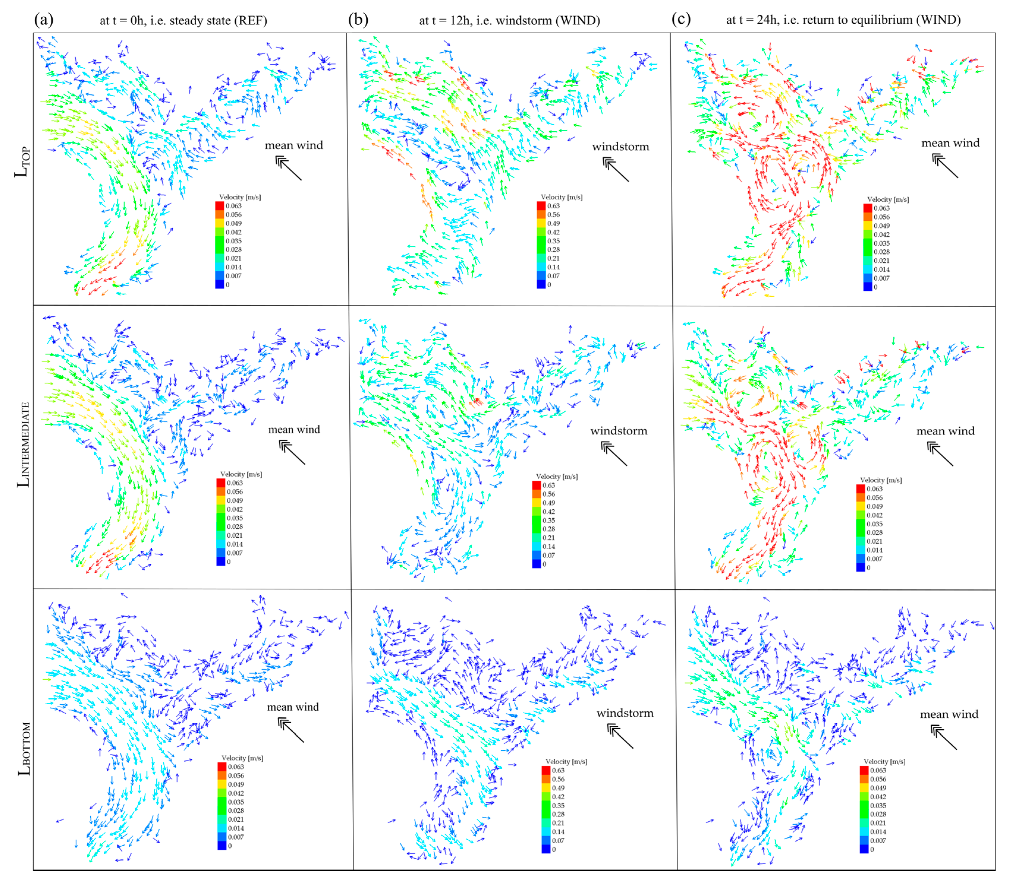
Figure 5.
Vertical output of the velocities in section SBORDER and profile in A-A for the different scenarios: in absence of wind (a), for REF (b), for WIND at t = 12 h (c) and at t = 5 d after the windstorm (d).
Figure 5.
Vertical output of the velocities in section SBORDER and profile in A-A for the different scenarios: in absence of wind (a), for REF (b), for WIND at t = 12 h (c) and at t = 5 d after the windstorm (d).

Figure 6.
Vertical output of the velocities in section SBAY for REF (a) and for (b) WIND at t = 12 h.
Figure 6.
Vertical output of the velocities in section SBAY for REF (a) and for (b) WIND at t = 12 h.

Figure 7.
Vertical output of the velocities in section SCHANNEL for (a) REF and for (b) WIND at t = 12 h.
Figure 7.
Vertical output of the velocities in section SCHANNEL for (a) REF and for (b) WIND at t = 12 h.
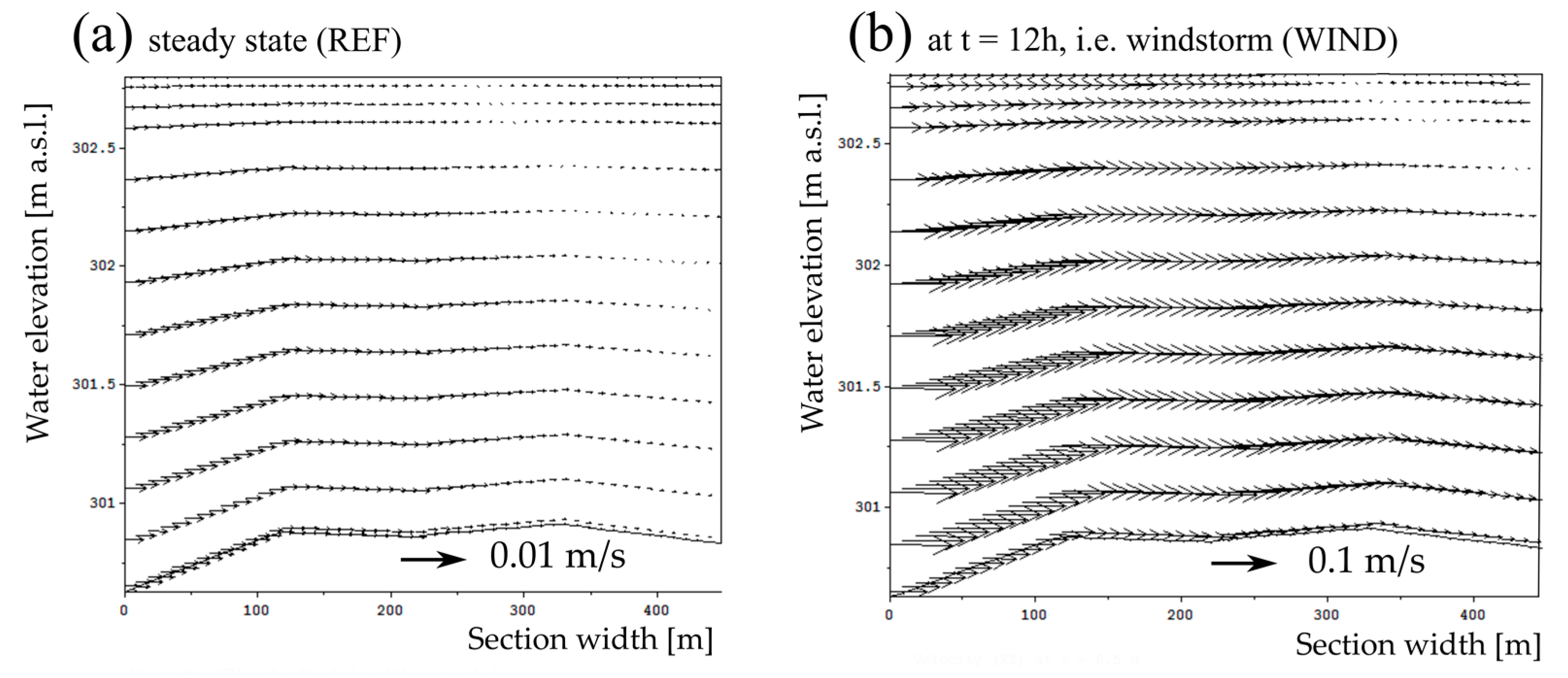
Figure 8.
Results of the HEAT scenario after one day simulation. The horizontal layers at the surface (LTOP), intermediate (LINTERMEDIATE) and bottom (LBOTTOM) are shown (respectively a,b,c).
Figure 8.
Results of the HEAT scenario after one day simulation. The horizontal layers at the surface (LTOP), intermediate (LINTERMEDIATE) and bottom (LBOTTOM) are shown (respectively a,b,c).

Figure 9.
Results of the HEAT scenario after one day simulation in section SBORDER (Figure 2 and Figure 5), showing the vertical configuration of temperatures and velocities over the vertical section. The arrows represent the velocity intensities and orientations in the section (water mass) and it is observable how they were more intense near the contour of the section next to the shores.
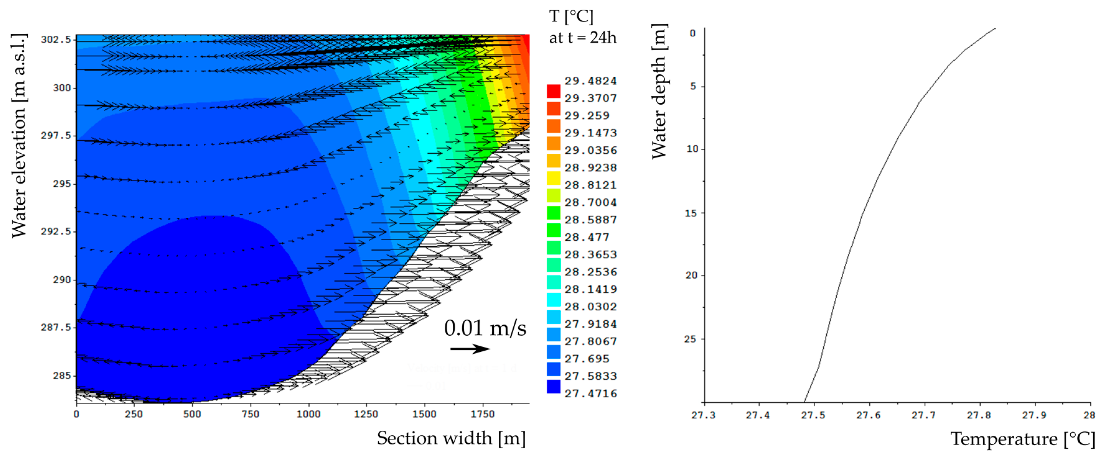
Figure 10.
Results of the HEAT scenario after one day simulation in section SBAY (Figure 2 and Figure 6), showing the vertical configuration of temperatures and velocities over the vertical section. The arrows represent the velocity intensities and orientations in the section (water mass).

Figure 11.
Results of the HEAT scenario after one day simulation in section SCHANNEL (Figure 2 and Figure 7), showing the vertical configuration of temperatures and velocities over the vertical section. The arrows represent the velocity intensities and orientations in the section (water mass).


Table 1.
Simulated scenarios and selected parameters (REF (reference), WIND and HEAT).
| Scenarios | Simulation | Period of the Day (h) | Wind Velocity [m/s] | Wind Direction [°] | Tracer Transport |
|---|---|---|---|---|---|
| REF | 10 days | 00:00–24:00 | 5.5 | 140 | Not included |
| WIND | 1 day | 00:00–09:00 | 5.5 | 140 | Not included |
| 09:00–15:00 | 20.0 | ||||
| 15:00–24:00 | 5.5 | ||||
| HEAT | 1 day, 1 week, 1 month | 00:00–24:00 | 5.5 | 140 | = 10 °C |
© 2017 by the authors. Licensee MDPI, Basel, Switzerland. This article is an open access article distributed under the terms and conditions of the Creative Commons Attribution (CC BY) license (http://creativecommons.org/licenses/by/4.0/).
Share and Cite
MDPI and ACS Style
Matta, E.; Selge, F.; Gunkel, G.; Hinkelmann, R. Three-Dimensional Modeling of Wind- and Temperature-Induced Flows in the Icó-Mandantes Bay, Itaparica Reservoir, NE Brazil. Water 2017, 9, 772. https://doi.org/10.3390/w9100772
AMA Style
Matta E, Selge F, Gunkel G, Hinkelmann R. Three-Dimensional Modeling of Wind- and Temperature-Induced Flows in the Icó-Mandantes Bay, Itaparica Reservoir, NE Brazil. Water. 2017; 9(10):772. https://doi.org/10.3390/w9100772
Chicago/Turabian StyleMatta, Elena, Florian Selge, Günter Gunkel, and Reinhard Hinkelmann. 2017. "Three-Dimensional Modeling of Wind- and Temperature-Induced Flows in the Icó-Mandantes Bay, Itaparica Reservoir, NE Brazil" Water 9, no. 10: 772. https://doi.org/10.3390/w9100772
Note that from the first issue of 2016, this journal uses article numbers instead of page numbers. See further details here.