Aquifer Vulnerability Assessment for Sustainable Groundwater Management Using DRASTIC

1
Sustainability Innovation Lab at Colorado (SILC), University of Colorado Boulder, Boulder, CO 80309, USA
2
Department of Agricultural & Biological Engineering, Purdue University, West Lafayette, IN 47907, USA
3
Department of Earth, Atmospheric, and Planetary Sciences, Purdue University, West Lafayette, IN 47907, USA
*
Author to whom correspondence should be addressed.
Water 2017, 9(10), 792; https://doi.org/10.3390/w9100792
Submission received: 2 September 2017
/
Revised: 8 October 2017
/
Accepted: 12 October 2017
/
Published: 15 October 2017
Abstract
:Groundwater management and protection has been facilitated by computational modeling of aquifer vulnerability and monitoring aquifers using groundwater sampling. The DRASTIC (Depth to water, Recharge, Aquifer media, Soil media, Topography, Impact of vadose zone media, and hydraulic Conductivity) model, an overlay and index GIS model, has been used for groundwater quality assessment because it relies on simple, straightforward methods. Aquifer vulnerability mapping identifies areas with high pollution potential that can be areas for priority management and monitoring. The objectives of this study are to demonstrate how aquifer vulnerability assessment can be achieved using DRASTIC with high resolution data. This includes calibrating DRASTIC weights using a binary classifier calibration method with a genetic algorithm (Bi-GA), identifying areas of high potential aquifer vulnerability, and selecting potential aquifer monitoring sites using spatial statistics. The aquifer vulnerability results from DRASTIC using Bi-GA were validated with a well database of observed nitrate concentrations for a study area in Indiana. The DRASTIC results using Bi-GA showed that approximately 42.2% of nitrate detections >2 ppm are within “High” and “Very high” vulnerability areas (representing 3.4% of study area) as simulated by DRASTIC. Moreover, 53.4% of the nitrate detections were within the “Moderate” vulnerability class (26.9% of study area), and only 4.3% of the nitrate detections were within the “Low” vulnerability class (60.1% of study area). Nitrates >2 ppm were not detected at all within the “Very low” vulnerability class (9.6% of area). “High” and “Very high” vulnerability areas should be regarded as priority areas for groundwater monitoring and efforts to prevent groundwater contamination. This case study suggests that the approach may be applicable to other areas as part of efforts to target groundwater management efforts.
1. Introduction
Despite its widespread use as drinking water globally, groundwater is a poorly understood resource [1]. Groundwater provides human populations with a variety of services, including water for drinking and irrigation. However, groundwater systems have been increasingly threatened, directly and indirectly, by human activities [2].
Groundwater is typically not easily contaminated, yet once this occurs water quality is difficult to restore. Furthermore, groundwater pollution is not visible and is detected only when a well or spring becomes noticeably polluted or the pollutant is discharged into surface waters [3]. Groundwater management is necessary to maintain clean groundwater. Groundwater management has usually been facilitated by either modeling aquifer vulnerability with computational models or monitoring aquifers using groundwater sampling.
Groundwater monitoring and sampling provide insight into groundwater quality and quantity directly in real time. A groundwater monitoring network can provide quantity and quality data necessary to make informed decisions regarding the state of the environment. A properly designed monitoring system provides a representative understanding of the state of the monitored area [4]. Groundwater monitoring and sampling, however, are complex, difficult to apply for broad areas, and costly. In addition, improper distribution of monitoring sites or an insufficient number of sites may result in an unrepresentative view of the state of the environment. On the other hand, if the sampled sites are too numerous, the information obtained is redundant and the monitoring network is costly and inefficient [4].
Compared with groundwater monitoring and sampling, groundwater modeling is less complex and costly, and allows evaluation of broad areas. Groundwater modeling can be used to select the optimal number of monitoring locations and their spatial distribution for detecting pollution in groundwater aquifers and can be useful to assess groundwater quality and provide a guide to manage groundwater efficiently [4,5,6]. However, if only modeling techniques are used, groundwater quality and quantity would be indirectly estimated and could not be calibrated and validated. Therefore, if monitoring is conducted after identifying the most vulnerable areas by modeling techniques as an initial screening tool, potential monitoring sites and areas where Best Management Practices (BMPs) for groundwater quality protection can be determined in an effective and economic manner [7].
Various groundwater models, such as MODFLOW (MODular Three-dimensional finite-difference groundwater FLOW model), GSFLOW (coupled Ground-water and Surface-water FLOW model), and GWM-2005 (GroundWater Management process for MODFLOW-2005) [8,9,10,11], have been used to evaluate groundwater quality. These models require significant input data to run, and for most users it is not easy to use the models because they are fairly complicated. Moreover, they have limitations in simulating large areas because they need many input data in ASCII format and much computation time according to many model cells. As an alternative, the DRASTIC (Depth to water, Recharge, Aquifer media, Soil media, Topography, Impact of vadose zone media, hydraulic Conductivity) model, an overlay/index GIS model, has been used by several researchers for efforts related to groundwater quality assessment because DRASTIC uses simple and straightforward methods [12,13].
The DRASTIC model has received some criticism due to limited validation. Holden et al. [14] and Maas et al. [15] reported little correlation between model results and field data. In spite of these concerns, DRASTIC has been widely used to evaluate environmental impacts associated with groundwater pollution based on different ratings criteria, and the strength of the vulnerability concept is that it is performed by classifying a geographical area in terms of its susceptibility to groundwater contamination [16,17,18]. Advantages of the DRASTIC model include the method’s low cost of application [18,19] and the relative accuracy of model results for extensive regions with a complex geological structure [20,21]. Moreover, DRASTIC requires limited input data and has small computational needs, because there is no complex numerical analysis that requires many parameters, and there is no complicated simulation process [22]. DRASTIC is a reconnaissance tool, but has proven its value as an indicator of areas deserving detailed hydrogeologic evaluation, and is useful as an initial screening tool to evaluate aquifer vulnerability in broad areas and priorities for monitoring [4]. For these reasons, DRASTIC was used in this study of aquifer vulnerability assessment and as a way to identify groundwater monitoring locations. Disadvantages of DRASTIC identified in previous studies were used here to drive modifications to improve estimation of aquifer vulnerability.
The objectives of this study are to: (1) conduct aquifer vulnerability assessment with DRASTIC using high resolution data; (2) calibrate DRASTIC weights using a binary classifier calibration with a genetic algorithm (Bi-GA); (3) identify areas that have potentially high aquifer vulnerability and select potential aquifer monitoring and management sites for effective monitoring planning and areas where BMPs to prevent groundwater contamination might be considered; and (4) evaluate the performance of this approach by comparing the vulnerability assessment with monitoring data. Our study area for this assessment is a large watershed in Indiana, USA, a state where approximately 60% of the drinking water is supplied by groundwater.
2. Materials and Methods
2.1. Study Area
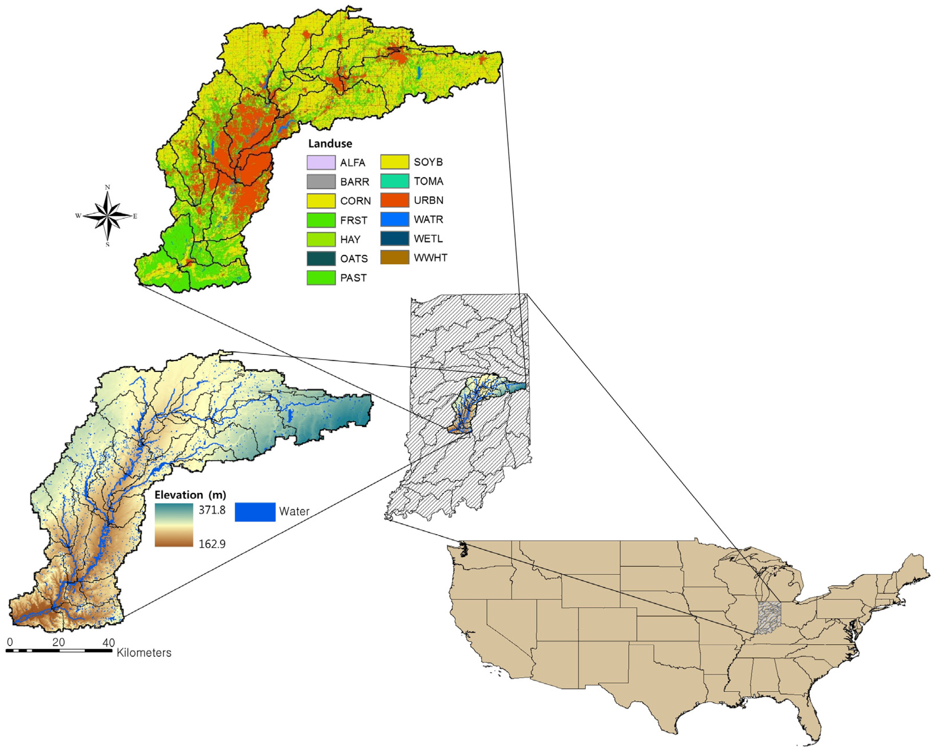
The study area (Figure 1) is the Upper White River Watershed (UWRW) (Latitude: 39°29′51″ N, Longitude: 86°24′02″ W), a Hydrologic Unit Code (HUC) 8 watershed (05120201) located in central Indiana and includes seventeen HUC 10 subwatersheds. Land Use and Land Cover (LULC) in the UWRW includes 45.5% agricultural (22.5% soybeans, 22.2% corn, and 0.8% others), 23.5% urban, 14.9% forest, 12.6% pasture, and 3.5% other LULC types.
The UWRW is important for public drinking water supplies as it includes more than 3508 km of streams, numerous artificial lakes, and 4 reservoirs. Sixteen counties are located in the watershed, and the UWRW serves as a portion of the drinking water supply for the city of Indianapolis, which is Indiana’s largest city. The water sources in the rural areas of UWRW traditionally are individual wells to provide groundwater for residential, commercial, and industrial purposes [23,24]. The UWRW was selected to evaluate the improved DRASTIC (ver.2015).
2.2. DRASTIC to Estimate Aquifer Vulnerability
Various groundwater vulnerability assessment approaches have been developed to evaluate aquifer vulnerability. These include process based methods, statistical methods, and overlay/index methods [25,26]. The process based methods use simulation models (i.e., SWAT [27], HSPF [28], and GLEAMS [29]) to simulate contaminant transport [22]. Statistical methods identify relationships between simulated results or spatial variables and observed data in the aquifer. The overlay/index methods (i.e., AVI (Aquifer Vulnerability Index) [30], COP (Concentration of flow, Overlying layer and Precipitation) [31], DRASTIC [19], GOD (Groundwater hydraulic confinement, aquifer Overlying strata resistivity, and Depth to water table) [32], and Irish [33]) are based on assembling information on the most relevant characteristics affecting aquifer vulnerability. Using overlay/index methods, aquifer vulnerability is evaluated by scoring, integrating, or classifying the information to produce an index, rank, or class of vulnerability [34]. The overlay/index methods are easy to apply, especially on regional or larger areas. Therefore, these are the most popular methods used in aquifer vulnerability assessment for various spatial scales (from local to global scale).
DRASTIC is a conceptual model defined as a composite description of the most important geological and hydrological factors that could potentially affect aquifer pollution. DRASTIC yields a numerical index map of groundwater vulnerability that is derived from ratings and weights assigned to the seven map parameters [18,19] (Equation (1)). The higher the DRASTIC index score, the greater the groundwater vulnerability. The smallest possible DRASTIC index is 23 and the largest is 230, if the range of DRASTIC weights ranges from 1 to 5.
where
- Dr: Ratings to the depth to water table;
- Dw: Weight assigned to the depth to water table;
- Rr: Ratings for ranges of aquifer recharge;
- Rw: Weight for aquifer recharge;
- Ar: Ratings assigned to aquifer media;
- Aw: Weight assigned to aquifer media;
- Sr: Ratings for soil media;
- Sw: Weight for soil media;
- Tr: Ratings for topography;
- Tw: Weight assigned to topography;
- Ir: Ratings assigned to vadose zone;
- Iw: Weight assigned to vadose zone;
- Cr: Ratings for rates of hydraulic conductivity; and
- Cw: Weight given to hydraulic conductivity.
With various DRASTIC weights, ranges, and ratings (Table A1), users can assign ratings and weights in determining D, R, A, S, T, I, and C maps. The variable rating allows users to select either a typical value or to modify the value based on users’ experience and knowledge in a specific area. The DRASTIC model was designed to allow users to make a flexible modification so that the local hydrogeological characteristics could be reflected and its parameters could be weighted properly [35].
DRASTIC has also been applied to many regions around the world. Babiker et al. [17] estimated aquifer vulnerability and demonstrated the combined use of DRASTIC and GIS in Kakamigahara Heights, Gifu Prefecture, Central Japan. They utilized sensitivity analyses to evaluate the relative importance of the model parameters for aquifer vulnerability. Navulur [16] developed a technique for estimating the vulnerability of groundwater to nitrate contamination from non-point sources (NPS) on a regional scale. In the study reported here, the technique was applied to evaluate vulnerability of groundwater systems in a large watershed in Indiana, United States, using a GIS environment with 1:250,000 scale data. Vulnerability of Indiana aquifer systems to NPS of pollution was also evaluated using DRASTIC and SEEPAGE (System for Early Evaluation of Pollution potential from Agricultural Groundwater Environments) analyses.
2.3. Sources of Data
In this study, most data for DRASTIC ver.2015 are at 1:24,000 scale (Table 1), unlike the 1:250,000 scale data for DRASTIC ver.1996. The data include water table depth, precipitation, evapotranspiration, LULC, aquifer systems, SSURGO used to produce recharge, soil media, and topography layers, lithology, and aquifer transmissivity data (Table 1).
2.4. Nitrate Measurements
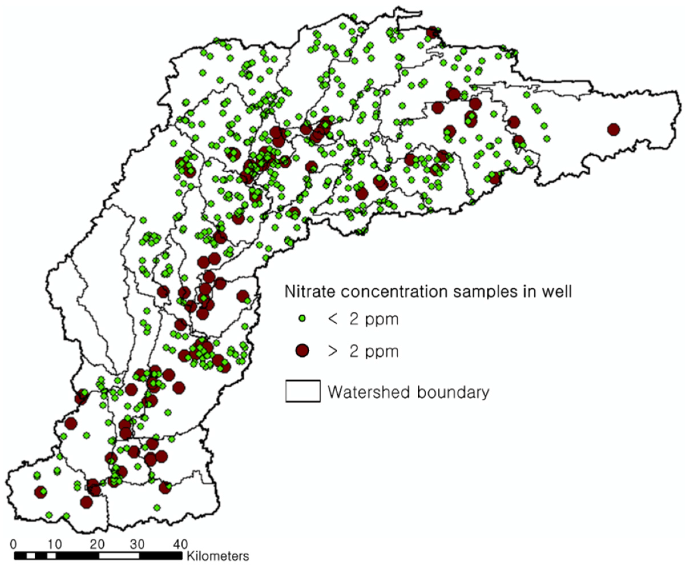
To calibrate the DRASTIC index map, nitrate concentration was selected as the contaminant parameter. Nitrate levels in groundwater under natural conditions are typically less than 2 ppm in Indiana. Nitrate detection >2 ppm has been assumed to be caused by human activities. Thus, a threshold value of background concentration was set at 2 ppm in this study [16]. One hundred sixteen wells (116 out of total 678 wells) (Figure 2) with nitrate levels >2 ppm (>2 mg/L) were selected to calibrate and validate estimated high aquifer vulnerability areas. Nitrate levels vary from 0.1 to 18.3 mg/L with an average of 1.2 mg/L in the study area.
2.5. Aquifer Vulnerability Mapping Using DRASTIC
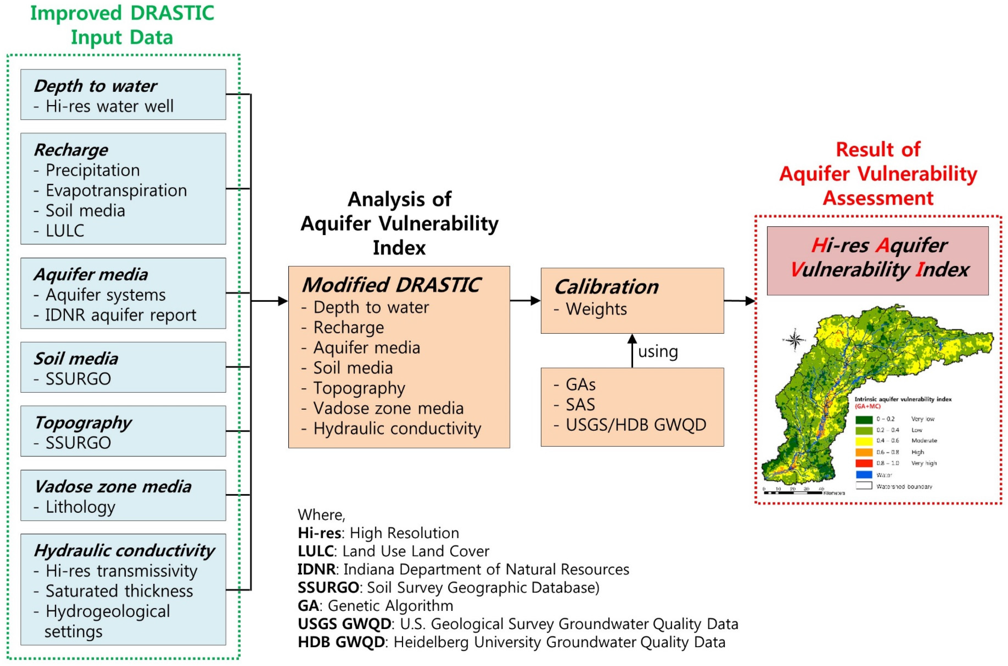
Methods described below were used for DRASTIC to create an aquifer vulnerability map. The seven map layers (Table 2), representing the seven parameters of DRASTIC, were prepared for the UWRW. DRASTIC ratings and weights were assigned to each map according to DRASTIC standards [36]. Then, weights were modified to reflect local characteristics for aquifer vulnerability maps. Finally, model calibration was conducted (Figure 3).
Aquifer vulnerability indices were divided into five classes (“Very low”, “Low”, “Moderate”, “High”, and “Very high” vulnerability classes) by normalization of DRASTIC indices using Equation (2). Feature scaling (data normalization) is a method used to standardize the range of independent variables (min = 0, max = 1). It is generally utilized during data preprocessing. The map resolutions of previous DRASTIC aquifer vulnerability maps usually are crude. In addition, DRASTIC parameters were optimized to adjust DRASTIC weights with a binary classifier calibration method with GA (hereafter referred to as Bi-GA). More description of Bi-GA is in Section 2.6.
The aquifer vulnerability map was created by combining the seven map layers after multiplying each map layer with its theoretical ratings and weights (Equation (1)). Then, calibration for DRASTIC weights was carried out. Two DRASTIC result maps with no calibration and calibration with Bi-GA had different ranges of DRASTIC vulnerability indices because different weight values were applied for each DRASTIC result map. Finally, optimized high resolution aquifer vulnerability predictions with calibrated DRASTIC weights were generated using the GIS spatial analyst tool.
where is the normalized value and is the original value.
2.5.1. Depth to Water
High spatial resolution long-term static water level data in wells (1990–2008 years) were utilized to obtain the “Depth to water” (D) map and interpolation was required. Minimum, maximum, and average depths to water are 3.1 m, 167.6 m, and 10.6 m, respectively. Kriging interpolation was used because this method is an effective way to interpolate a limited number of observations for hydrologic properties, such as rainfall, aquifer characteristics, effective recharge and to preserve the theoretical spatial correlation [37]. Then, interpolated data were reclassified into ratings according to Appendix A Table A1.
2.5.2. Recharge
Land uses/land covers (LULCs) and soils are sensitive parameters in calculating the amount of recharge. To consider regional LULC and soil characteristics, the Soil Conservation Service (SCS) runoff curve number (CN) method was used to estimate potential recharge with precipitation, soils and LULCs [38,39]. Potential recharge was computed as precipitation minus surface runoff which is determined by the SCS-CN method. Potential recharge estimated in this study may not reflect the actual amount of recharge but rather indicates possible recharge rate. Estimation of potential recharge (potential infiltration rate) ignored evapotranspiration (ET) because ET occurs after infiltration. Thus, even though there is a limitation in ignoring ET when calculating potential recharge, this approach for estimating potential recharge has been used in DRASTIC [38,39,40,41]. Precipitation data from National Climate Data Center (NCDC), LULC data from National Land Cover Database (NLCD) and soil data (SSURGO) from Natural Resources Conservation Service (NRCS) were used to produce a potential recharge map using the SCS-CN method (Equation (3)). Then, a DRASTIC rating for annual potential recharge was determined using Table A1 [40,41]. When detailed recharge estimation is needed for small areas with DRASTIC, the approach to estimating recharge suggested in this study would be more useful than other studies [13,17], which calculates the amount of recharge using only two LULC classes (e.g., urban and remaining areas).
where
- Qi: Depth of runoff (mm);
- P: Depth of rainfall (mm);
- Ia: Initial abstraction (mm);
- S: Maximum potential retention (mm); and
- CN: Curve number (dimensionless).
2.5.3. Aquifer Media
An “Aquifer media” (A) map was created using the aquifer systems map and report by the U.S. Geological Survey (USGS) and the Indiana Department of Natural Resources (IDNR). Most aquifer media in the study area were sand and gravel, but, based on the INDR reports, an aquifer media rating was assigned in more detail [42]. IDNR reports of counties in Indiana described vulnerability of each aquifer system such as “very high susceptibility to surface contamination (very high)”, “highly susceptible to surface contamination (high)”, “moderately susceptible to surface contamination (moderate)”, “low susceptibility to surface contamination (low)”, and “very low susceptibility to surface contamination (very low)”. Vulnerability ratings were divided into five levels (very high = 10, high = 8, moderate = 6, low = 4, and very low = 2). Then, modified reclassification of ratings was conducted as shown in Table 3.
2.5.4. Soil Media and Topography
“Soil media” (S) and “Topography” (T) maps were obtained through SSURGO data from USDA-NRCS instead of STATSGO data often used. The map scale of SSURGO data is 1:12,000, whereas STATSGO is 1:250,000. Of many fields of the SSURGO table, “MUNAME” is needed to analyze DRASTIC S and required information is a soil type (e.g., loam, silt loam, and sandy loam). However, a MUNAME field in the original SSURGO table describes detailed soil type such as “Martinsville loam, 1 to 5 percent slopes”, “Jasper silt loam, 1 to 5 percent slopes”. This detailed information is unnecessary for DRASTIC ratings, because extracting only soil type of a number of fields is time-consuming. Therefore, a database to produce DRASTIC S was constructed using GIS and Python programming, and DRASTIC S and T maps were generated using a modified SSURGO data table. The S and T maps have ratings as described in Table A1.
2.5.5. Impact of Vadose Zone Media
“Impact of vadose zone media” (I) map was estimated using sand, silt, and clay thickness point data within lithology data from IDNR. Kriging interpolation was used to estimate unknown areas with known data points, and DRASTIC ratings were assigned according to Table A1.
2.5.6. Hydraulic Conductivity
The “Hydraulic Conductivity” (C) map (Equation (4)) was calculated with high resolution transmissivity (1:24,000) and saturated thickness data from IDNR based on hydrogeological settings. The C map was then reclassified into ranges and assigned ratings from 1 to 10 according to Table A1. Regions with higher hydraulic conductivity have a greater possibility of contamination.
Hydraulic conductivity (m/s) = Transmissivity (m2/s)/Thickness of aquifer (m)
2.6. Model Calibration and Validation
Probabilistic predictive or decision-making models (i.e., DRASTIC and SEEPAGE) need pre-processing prior to calibration with observed data because results of probabilistic predictive or decision-making models have different scale or format than observed data that are used for model calibration [43,44]. Thus, in this study, a binary classifier calibration method was combined with a genetic algorithm (Bi-GA) and used for calibration of DRASTIC weights. In the binary classifier calibration, results of model and observed data are classified as 0 or 1. DRASTIC produces five vulnerability classes (i.e., very high, high, moderate, low, and very low). This study classified very high and high vulnerability classes as 1 and other classes as 0. In addition, observed nitrate concentrations over 2 ppm and below 2 ppm in wells are assigned as 1 and 0, respectively, because nitrate detections >2 ppm were used in DRASTIC calibration.
Bi-GA was utilized for calibration of DRASTIC weights using Heidelberg University and USGS groundwater quality data which are mean nitrate concentration data from 81 wells with nitrate levels >2 ppm, which is the threshold value for the background concentration level of nitrate. Calibration with Bi-GA was conducted to improve the performance of the DRASTIC model. Original DRASTIC weights vary from 1 to 5 (Table 2). Based on original DRASTIC weights, Depth to water (D) and Impact of vadose zone (I) are the most sensitive parameters, and the second most sensitive parameter is Recharge (R) in assessing an aquifer vulnerability. However, in many studies using DRASTIC, original relationships of DRASTIC weights between the seven map layers have been ignored in the calibration process. For this study, even though calibrated DRASTIC weights were different from original values, the ratio of DRASTIC weights (5 (D), 4 (R), 3 (A), 2 (S), 1 (T), 5 (I), and 3 (C)) was maintained. The Bi-GA modified the ratio of DRASTIC weights based on calibrated weights with Bi-GA, and there are weight boundaries which are ±1 from original DRASTIC weights. For instance, maximum and minimum weight values of D are 6 and 4. Based on calibrated weights by the Bi-GA which ignored the original DRASTIC weight relationships between the seven map layers, new calibrated weights which consider the ratio of DRASTIC weights (5 (D), 4 (R), 3 (A), 2 (S), 1 (T), 5 (I), and 3 (C)) were generated by: (1) no calibration; and (2) calibration with Bi-GA. Root mean square error (RMSE) was used to evaluate the effectiveness of the Bi-GA and its ability to make predictions in the calibration procedure. Lower RMSE values indicate a better fit. RMSE is a statistical measure of how accurately the model predicts observed nitrate over 2 ppm. In the calibration process, GA was used to minimize RMSE by adjusting DRASTIC weights (Equation (5)). The GA driving variables used in this study are shown in Table 4.
An accuracy assessment error matrix was computed to validate the results using 35 wells with nitrate levels >2 ppm following calibration using Bi-GA. Using an accuracy assessment error matrix, spatial patterns in success (detections of nitrate concentration in wells over 2 ppm) and failure (detections of nitrate concentration in wells under 2 ppm) of DRASTIC prediction were analyzed with a total accuracy measure.
where
- : Simulated nitrate concentration DRASTIC binary value; and
- : Observed nitrate concentration binary value.
2.7. Evaluation for Potential Groundwater Monitoring Sites
Hotspot analysis using the Getis–Ord Gi* (Gi*) [45,46] was applied to select potential groundwater monitoring sites. This method works by examining each feature (each grid cell) within the context of neighboring features. If a feature has a high value (high DRASTIC vulnerability index) and is surrounded by other features with high values, this feature is defined as a hotspot with statistical significance. The Gi* statistic returned for each feature in the dataset is a z-score. For statistically significant positive z-scores, the larger the z-score, the more intense the clustering of high values (hotspot) [47]. Thus, potential groundwater monitoring sites (where aquifer may be the most vulnerable to contamination) would be found based on the z-score with statistical significance. The hotspot analysis using the Gi* statistic was conducted using Equations (6)–(8) with the GIS spatial analyst tool.
where
- : Getis–Ord local statistic;
- : Attribute value for feature j;
- : Spatial weight between feature i and j; and
- : Total number of features.
3. Results and Discussion
3.1. Calibration and Validation of DRASTIC Weights
As shown in Table 5, RMSE for aquifer vulnerability without calibration was 0.70. The RMSE for aquifer vulnerability with calibrated DRASTIC parameters using Bi-GA was 0.57. RMSE for Bi-GA might be decreased (the lower RMSE, the better performance) because calibrated DRASTIC weights using Bi-GA maintained the ratios of original DRASTIC weights. Previous studies did not maintain the ratios of original DRASTIC weights to improve just performance evaluation of DRASTIC. However, if the ratios of original DRASTIC weights are not maintained, the number of degrees of freedom of the DRASTIC index (result scores for aquifer vulnerability) would be increased by calibrating DRASTIC weights. Further, physical properties for aquifer vulnerability could potentially be ignored.
For validation of the results by using Bi-GA, accuracy assessment was computed with 35 wells with nitrate levels > 2 ppm. As shown in the Table 6, total accuracies of uncalibrated DRASTIC and calibrated DRASTIC were 34% (=12/35) and 46% (=16/35), respectively. Thus, the results of accuracy assessment indicate calibrated DRASTIC predicted aquifer vulnerability areas contaminated by human activities more accurately than uncalibrated DRASTIC.
DRASTIC, an overlay and index GIS model, does not compute nitrate concentrations in aquifers, rather it predicts aquifer vulnerability classes from very high vulnerability to very low vulnerability. This study assumed nitrate concentrations greater than 2 ppm were caused by human activities and over 2 ppm of nitrate concentrations should typically be detected in “High” and “Very high” vulnerability classes. Thus, the greater the proportion of nitrate detections >2 ppm in “High” and “Very high” vulnerability areas, the better the prediction of aquifer vulnerability. If “High” and “Very high” vulnerability areas as a percentage are larger than number of nitrate detections >2 ppm as a percentage, the model performance should be regarded as poor, which would be overestimated by DRASTIC. This is captured in the concept of a detection ratio (percent of nitrate detections >2 ppm to percent of “Very high” and “High” vulnerability areas) with larger detection ratios indicating better prediction used to evaluate model performance in this study.
3.2. Aquifer Vulnerability Mapping
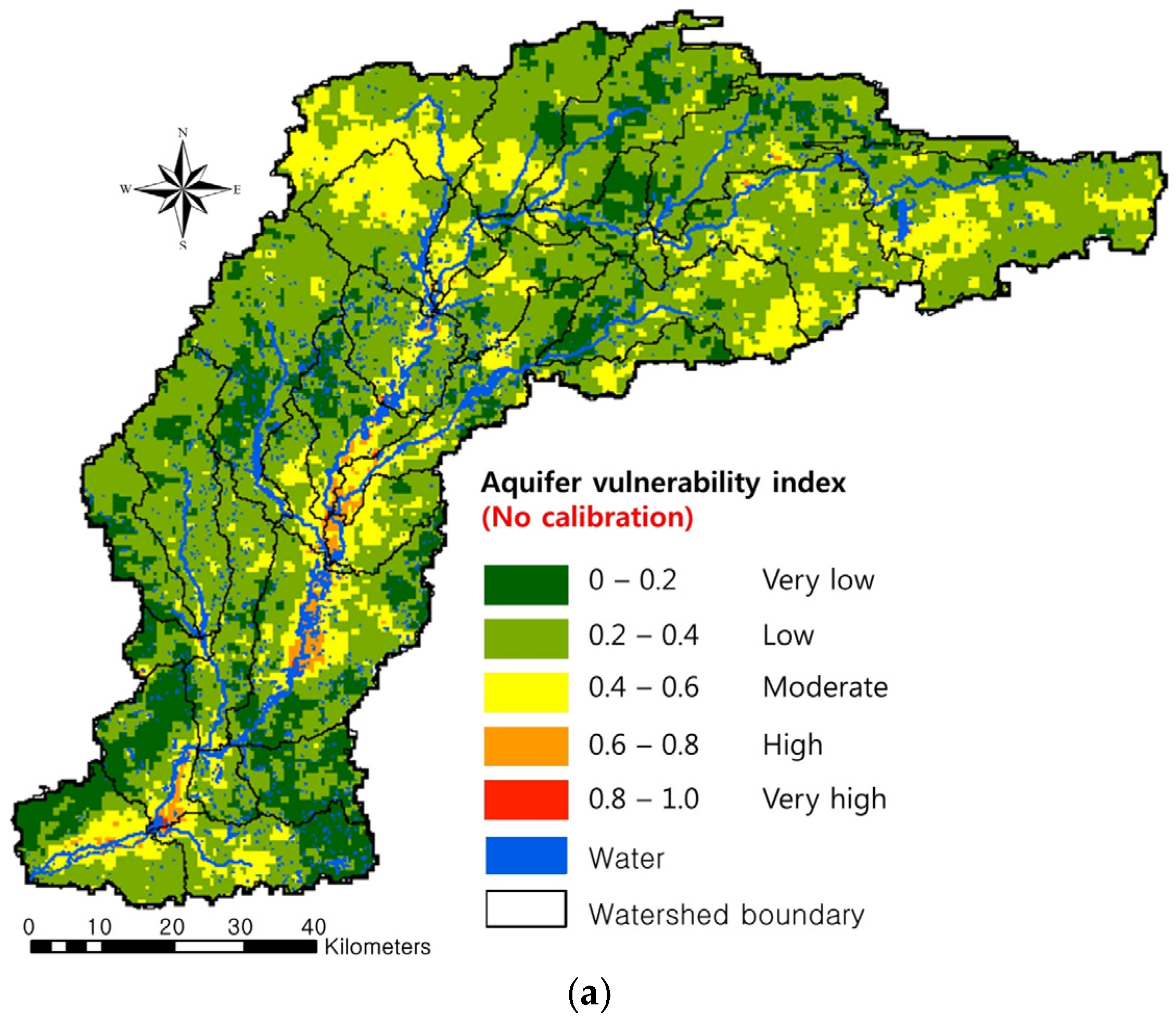
An aquifer vulnerability map without calibrating DRASTIC weights was created using DRASTIC (Figure 4a). Aquifer vulnerability indices were classified into five classes: 0–0.2 (“Very low”), 0.2–0.4 (“Low”), 0.4–0.6 (“Moderate”), 0.6–0.8 (“High”), and 0.8–1.0 (“Very high”). As shown in Figure 4a and Table 7, 10.6% of the aquifer systems in the UWRW were within in “Very low” vulnerability class, and 60.4% of the area was estimated as “Low”, 25.8% within “Moderate” vulnerability class, 3.0% within “High” vulnerability class, and 0.2% within “Very high” vulnerability class.
The aquifer vulnerability results (Table 7) without calibration of DRASTIC weights were validated with the observed nitrate concentrations in wells. The results showed that approximately 35.3% of nitrate detections >2 ppm were within “High” and “Very high” vulnerability areas (represent 3.2% of vulnerability area) as simulated by DRASTIC. Moreover, 60.3% of the nitrate detections were within the “Moderate” vulnerability class (25.8% of area), 3.4% of the nitrate detections were within the “Low” vulnerability class (60.4% of area), and 0.9% of the nitrate detections were within the “Low” vulnerability class (10.6% of area) (Table 7).
An aquifer vulnerability map with calibrated DRASTIC using Bi-GA was produced (Figure 4b). As shown in Figure 4b and Table 8, 9.6% of the aquifer systems in the UWRW was within the “Very low” vulnerability class, and 60.1% of the area was estimated as “Low”, 26.9% within the “Moderate” vulnerability class, 3.2% within the “High” vulnerability class, and 0.2% within the “Very high” vulnerability class.
The aquifer vulnerability results (Table 8) from calibrated DRASTIC were validated with the well database. The results showed that approximately 42.2% of nitrate detections >2 ppm were within “High” and “Very high” vulnerability areas (represent 3.4% of vulnerability area) as simulated by DRASTIC. Moreover, 53.4% of the nitrate detections were within the “Moderate” vulnerability class (26.9% of area), and 4.3% of the nitrate detections were within the “Low” vulnerability class (60.1% of area). In aquifer vulnerability assessment, nitrates in wells >2 ppm were not detected within the “Very low” vulnerability class (9.6% of area) (Table 8). These results indicated that aquifer vulnerability assessment using DRASTIC with Bi-GA better predicted nitrate detections than DRASTIC without calibration.
Very high and high vulnerability areas were located along the stream and river because those areas include highly permeable alluvium, sand, and gravel. Further, depth to water is shallow and the vadose zone media includes gravel, sand, and peat. According to the land use map, very high and high vulnerability classes include areas that are mainly near streams, agricultural fields, and urban areas because fertilizer and urban organic wastes from these areas infiltrate toward aquifers. Based on the topography map, very high and high vulnerability classes are mainly observed in lowland areas where it is common to find agricultural lands that receive fertilizers and urban complexes that contribute in various ways to pollution.
This study assumed that nitrate concentrations in wells >2 ppm should have not been detected in “Low” and “Very low” vulnerability areas. However, five nitrate concentrations in wells >2 ppm (4.3% of total nitrate detections >2 ppm) were found in “Low” and “Very low” vulnerability areas. Four main reasons (groundwater age, point sources, wells that have failed, and groundwater flow) explain why detections may have occurred in “Low” and “Very low” vulnerability areas as these factors are not considered in DRASTIC.
GIS-based overlay and index models such as DRASTIC can be affected by data resolution and accuracy [48]. Navulur [16] used three models (i.e., DRASTIC, SEEPAGE, and combined DRASTIC and NLEAP (Nitrate Leaching and Economic Analysis)) to estimate aquifer vulnerability of groundwater systems in Indiana using a GIS environment at a 1:250,000 scale. The data scale used in Navulur’s [16] study was coarse (1:250,000) for field scale simulations. However, in this study, high resolution data (1:24,000) were used by data preprocessing of recharge (R), aquifer media (A), soil media (S), topography (T), and impact of vadose zone media (I) maps.
As shown in Navulur’s [16] results for all of Indiana, the result of DRASTIC shows 80.7% of nitrate detections in wells >2 ppm are within “High” and “Very high” vulnerability areas (represent 24.8% of area) as predicted by DRASTIC. For SEEPAGE, 60.5% of nitrate detections in wells >2 ppm are within “High” and “Very high” vulnerability areas (28.6% of area). The result of the combined DRASTIC and NLEAP indicate 91.8% of nitrate detections in wells >2 ppm are within “High” and “Very high” vulnerability areas (56.9% of area).
Compared with Navulur’s [16] study, the results presented herein had approximately 42.2% of nitrate detections in wells >2 ppm within “High” and “Very high” (3.4% of area) vulnerability areas as predicted by DRASTIC with high resolution data. Detection ratio (% of nitrate detections to % of vulnerability areas with larger detection ratio indicating better prediction) for “High” and “Very high” areas from Navulur’s [16] study results in a value of 3.3 for DRASTIC, 2.1 for SEEPAGE, and 1.6 for the combined DRASTIC and NLEAP. In contrast to the three models from Navulur’s [16] results, the results presented herein provide a value of 12.4. Thus, the detection ratio results indicate that DRASTIC with high resolution data may estimate areas of “High” and “Very high” vulnerability classes more accurately than models with coarse resolution data (Table 9).
3.3. Potential Groundwater Monitoring and Management Sites
The Gi* statistic method was used to determine potential groundwater monitoring and management sites. Three ranges of z-scores (1.65–1.96, 1.96–2.58, and >2.58) indicate potential groundwater monitoring and management sites (hotspots). Hotspots were predicted based on the z-score with statistical significance using the Gi* statistic method. The Gi* statistic method identifies statistically significant spatial clusters of high values (high vulnerability areas) and low values (low vulnerability areas). The Gi* statistic method returns a z-score and the higher the z-score, the stronger the intensity of the clustering.
In Table 10 and Figure 5, z-scores of hotspot analysis maps to identify potential groundwater monitoring sites were estimated using calibrated DRASTIC by Bi-GA. Higher z-scores and red color (potential vulnerability areas) in the maps (Table 10 and Figure 5) indicate hotspots which suggest priority areas for groundwater monitoring and management. The portion of the study area with a z-score ≥ 1.65 for Bi-GA is 19.9% (percentage of study area, 6944 km2), suggesting areas where groundwater monitoring and BMPs for groundwater quality might be considered. In Figure 5, hotspot areas (z-score ≥ 1.65) were located along the stream and river because those areas include highly permeable alluvium, sand, and gravel. Further, depth to water is shallow. These areas would be priorities for groundwater protection.
4. Conclusions
Aquifer vulnerability assessment was conducted with improved high resolution data and optimized DRASTIC parameters by modifying DRASTIC weights using Bi-GA. Simulated results to explore the most vulnerable aquifer areas estimated by DRASTIC were compared with Heidelberg University and USGS groundwater quality data (nitrate concentrations in wells) (1949–2010) in the UWRW, Indiana. Aquifer vulnerability indices from improved DRASTIC were compared with observed groundwater quality data to explore how well simulated results predict observed nitrate data >2 ppm. RMSE without calibration was 0.70, and RMSE with calibrating DRASTIC weights with Bi-GA was 0.57.
An accuracy assessment error matrix was computed for spatial validation of the calibrated DRASTIC by using Bi-GA. Total accuracies of uncalibrated DRASTIC and calibrated DRASTIC were 34% and 46%, respectively. Thus, the results of accuracy assessment indicate calibrated DRASTIC using Bi-GA predicted aquifer vulnerability areas were more accurate than DRASTIC without calibration.
The aquifer vulnerability results from DRASTIC using Bi-GA were validated with a well database. The results showed that approximately 42.2% of nitrate detections >2 ppm are within “High” and “Very high” vulnerability areas (represent 3.4% of vulnerability area) as estimated by DRASTIC. Moreover, 53.4% of the nitrate detections were within the “Moderate” vulnerability class (26.9% of area), and 4.3% of the nitrate detections were within the “Low” vulnerability class (60.1% of area). In aquifer vulnerability assessment, nitrates in wells > 2 ppm were not detected within the “Very low” vulnerability class (9.6% of area). Aquifer vulnerability assessment using calibration with Bi-GA better predicted nitrate detections than DRASTIC without calibration.
The selection of potential monitoring locations and areas where groundwater protection should be focused was determined based on the Gi* statistic method. A portion of z-score over 1.65 by Bi-GA is 19.9% (represents percentage area of total study area, 6944 km2), indicating these are areas where groundwater monitoring and BMPs for groundwater quality protection should be focused. Hotspot areas (z-score ≥ 1.65) were seen along the stream and river because those areas include high permeability of alluvium, sand, and gravel. Further, depth to water is shallow. These areas would be priorities for groundwater protection.
The results of this type of study can be used in managing groundwater resources by policy makers, natural resources protection practitioners, and groundwater-related researchers. It also can be used as a screening tool prior to applying complex numerical groundwater models for more detailed analysis. Moreover, it is expected that better parameterization of DRASTIC input data related to aquifer systems will improve aquifer vulnerability assessment and be applicable to other locations in the Midwestern, United States.
DRASTIC is not a numerical model to compute nitrate concentrations in aquifers but to predict aquifer vulnerability classes from very high vulnerability to very low vulnerability with hydrogeological settings. Thus, this study developed a new calibration method (Bi-GA) and new evaluation criteria of model performance called “detection ratio” for more accurate aquifer vulnerability assessment. Based on this study, we suggest that Bi-GA and the detection ratio would be an appropriate calibration method for DRASTIC and may improve model performance for those who use an overlay and index model.
This study has several limitations that could be addressed in future studies.
- (1)
- About 79% of land uses (45.5% agricultural and 23.5% urban areas) are human-related areas, and most human-related areas cover very high and high vulnerability classes. Thus, DRASTIC in this study describes human impact. For more accurate estimation of human impact by DRASTIC or other overlay and index models, more human-impact-related factors such as land use, population density, and point sources should be considered as input data.
- (2)
- For a detailed vulnerability assessment, the aquifer vulnerability analysis of DRASTIC would need to be combined with predictive models for pollutant transport. This combination is required to evaluate the actual quantitative risk. For example, models such as SWAT which can estimate pollutant transport could be combined with DRASTIC. Further, pollutant transport should be considered beyond that on the land surface and consider subsurface transport. To do this, more detailed soil data that describe various soil components for the surface and subsurface soil layers should be used for future study.
- (3)
- The aquifer vulnerability index is a combination of data. Further, there are many pre-processes and post-processes to generate an aquifer vulnerability index. Thus, an aquifer vulnerability index includes some degree of uncertainty which might come from data, data processing errors by the modeler, and model structure. Future work would benefit from quantification of errors when using an overlay and index model.
Author Contributions
Won Seok Jang designed the research, conducted data analysis, and wrote the paper. Bernard Engel and Jon Harbor contributed to the discussion and writing of the paper. Larry Theller conducted data collection and analysis.
Conflicts of Interest
The authors declare no conflict of interest.
Appendix A

Table A1.
Typical DRASTIC ranges and ratings.
| Depth to Water (m) | |
| Range | Rating |
| 0–1.5 | 10 |
| 1.5–4.6 | 9 |
| 4.6–6.8 | 8 |
| 6.8–9.1 | 7 |
| 9.1–12.1 | 6 |
| 12.1–15.2 | 5 |
| 15.2–22.9 | 4 |
| 22.9–26.7 | 3 |
| 26.7–30.5 | 2 |
| 30.5+ | 1 |
| Net Recharge (mm/year) | |
| Range | Rating |
| 254+ | 10 |
| 235–254 | 9 |
| 216–235 | 8 |
| 178–216 | 7 |
| 147.6–178 | 6 |
| 117.2–147.6 | 5 |
| 91.8–117.2 | 4 |
| 71.4–91.8 | 3 |
| 51–71.4 | 2 |
| 0–51 | 1 |
| Aquifer Media | |
| Range | Rating |
| Karst limestone | 10 |
| Basalt | 9 |
| Sand and gravel | 8 |
| Massive sandstone Massive limestone | 7 |
| 7 | |
| Bedded sandstone Limestone | 6 |
| 6 | |
| Glacial till | 5 |
| Weathered metamorphic igneous | 4 |
| Metamorphic igneous | 3 |
| Massive shale | 2 |
| Soil Media | |
| Range | Rating |
| Thin or absent/Gravel | 10 |
| Sand | 9 |
| Peat | 8 |
| Shrinking clay | 7 |
| Loamy sand | 6 |
| Sandy loam | 6 |
| Loam | 5 |
| Sandy clay | 4 |
| Sandy clay loam | 4 |
| Silt loam | 4 |
| Silty clay | 3 |
| Clay loam | 3 |
| Silty clay loam | 3 |
| Muck | 2 |
| Non-shrinking clay | 1 |
| Topography (%) | |
| Range | Rating |
| 0–2 | 10 |
| 2–6 | 9 |
| 6–12 | 5 |
| 12–18 | 3 |
| 18+ | 1 |
| Vadose Zone Media | |
| Range | Rating |
| Thin or absent/Gravel | 10 |
| Sand | 9 |
| Peat | 8 |
| Shrinking clay | 7 |
| Loamy sand | 6 |
| Sandy loam | 6 |
| Loam | 5 |
| Sandy clay | 4 |
| Sandy clay loam | 4 |
| Silt loam | 4 |
| Silty clay | 3 |
| Clay loam | 3 |
| Silty clay loam | 3 |
| Muck | 2 |
| Non-shrinking clay | 1 |
| Hydraulic Conductivity (m/s) | |
| Range | Rating |
| 0.00095+ | 10 |
| 0.0005–0.00095 | 8 |
| 0.00033–0.0005 | 6 |
| 0.00015–0.00033 | 4 |
| 0.00005–0.00015 | 2 |
| 0.00000015–0.00005 | 1 |
References
- Solly, W.B.; Pierce, R.R.; Perlman, H.A. Estimated Use of Water in the United States in 1995; U.S. Geological Survey Circular 1200; USGS: Denver, CO, USA, 1998. [Google Scholar]
- Hamblin, W.K.; Christiansen, E.H. Earth’s Dynamic Systems, 10th ed.; Prentice Hall: Upper Saddle River, NJ, USA, 2004. [Google Scholar]
- Novotny, V. Water Quality, Diffuse Pollution and Watershed Management, 2nd ed.; Wiley: Van Nostrand Reinhold, NY, USA, 2003. [Google Scholar]
- Baalousha, H. Assessment of a groundwater quality monitoring network using vulnerability mapping and geostatistics: A case study from Heretaunga Plains, New Zealand. Agric. Water Manag. 2010, 97, 240–246. [Google Scholar] [CrossRef]
- Zhang, Y.; Li, G. Long-Term Evolution of Cones Depression in shallow Aquifers in the North China Plain. Water 2013, 5, 677–693. [Google Scholar] [CrossRef]
- Keilholz, P.; Disse, M.; Halik, Ü. Effects of Land Use and Climate Change on Groundwater and Ecosystems at the Middle Reaches of the Tarim River Using the MIKE SHE Integrated Hydrological Model. Water 2015, 7, 3040–3056. [Google Scholar] [CrossRef]
- Fienen, M.N.; Hunt, R.J.; Doherty, J.E.; Reeves, H.W. Using Models for the Optimization of Hydrologic Monitoring; U.S. Geological Survey Fact Sheet 2011–3014; USGS: Reston, VA, USA, 2011.
- McDonald, M.G.; Harbaugh, A.W. A Modular Three-Dimensional Finite-Difference Ground-Water Flow Model; US Geological Survey Techniques of Water Resources Investigations Report Book 6; USGS: Washington, DC, USA, 1988; Chapter A1.
- Lin, Y.-P.; Chen, Y.-W.; Chang, L.-C.; Yeh, M.-S.; Huang, G.-H.; Petway, J.R. Groundwater Simulations and Uncertainty Analysis Using MODFLOW and Geostatistical Approach with Conditioning Multi-Aquifer Spatial Covariance. Water 2017, 9, 164. [Google Scholar] [CrossRef]
- Harbaugh, A.W. MODFLOW-2005, The U.S. Geological Survey Modular Ground-Water Model-the Ground-Water Flow Process; U.S. Geological Survey Techniques and Methods 6-A16; USGS: Reston, VA, USA, 2005.
- Markstrom, S.L.; Niswonger, R.G.; Regan, R.S.; Prudic, D.E.; Barlow, P.M. GSFLOW-Coupled Ground-Water and Surface-Water FLOW Model Based on the Integration of the Precipitation-Runoff Modeling System (PRMS) and the Modular Ground-Water Flow Model (MODFLOW-2005); U.S Geological Survey, Techniques and Methods 6-D1; USGS: Reston, VA, USA, 2008.
- Pacheco, F.A.L.; Fernandes, L.F.S. The multivariate statistical structure of DRASTIC model. J. Hydrol. 2013, 467, 442–459. [Google Scholar] [CrossRef]
- Chen, S.; Jang, C.; Peng, Y. Developing a probability-based model of aquifer vulnerability in an agricultural region. J. Hydrol. 2013, 486, 494–504. [Google Scholar] [CrossRef]
- Holden, L.R.; Graham, J.A.; Whitmore, R.W.; Alexander, W.J.; Pratt, R.W.; Liddle, S.F.; Piper, L.L. Results of the national alachlor well water survey. Environ. Sci. Technol. 1992, 26, 936–943. [Google Scholar] [CrossRef]
- Maas, R.P.; Kucken, D.J.; Patch, S.C.; Peek, B.T.; Van Engelen, D.L. Pesticides in eastern North Caroline rural supply wells: Landuse factors and persistence. J. Environ. Qual. 1995, 24, 426–431. [Google Scholar] [CrossRef]
- Navulur, K.C.S. Groundwater Vulnerability Evaluation to Nitrate Pollution on a Regional Scale Using GIS. Ph.D. Dissertation, Purdue University, West Lafayette, IN, USA, 1996. [Google Scholar]
- Babiker, I.S.; Mohamed, M.A.A.; Hiyama, T.; Kato, K. A GIS based DRASTIC model for assessing aquifer vulnerability in Kakamigahara Heights, Gifu Prefecture, central Japan. Sci. Total Environ. 2005, 345, 127–140. [Google Scholar] [CrossRef] [PubMed]
- Akhavan, S.; Mousavi, S.; Abedi-Koupai, J.; Abbaspour, K.C. Conditioning DRASTIC model to simulate nitrate pollution case study: Hamadan-Bahar plain. Environ. Earth Sci. 2011, 63, 1155–1167. [Google Scholar] [CrossRef]
- Aller, L.; Bennett, T.; Lehr, J.H.; Petty, R.J.; Hackett, G. DRASTIC: A Standardized System for Evaluating Groundwater Potential Using Hydrogeologic Settings; EPA/600/2-85/018; U.S. Environmental Protection Agency: Washington, DC, USA, 1987.
- Kalinski, R.J.; Kelly, W.E.; Bogardi, I.; Ehrman, R.L.; Yamamoto, P.O. Correlation between DRASTIC vulnerabilities and incidents of VOC contamination of municipal wells in Nebraska. Ground Water 1994, 32, 31–34. [Google Scholar] [CrossRef]
- McLay, C.D.A.; Dragden, R.; Sparling, G.; Selvarajah, N. Predicting groundwater nitrate concentrations in a region of mixed agricultural land use: A comparison of three approaches. Environ. Pollut. 2001, 115, 191–204. [Google Scholar] [CrossRef]
- Barbash, J.E.; Resek, E.A. Pesticides in Ground Water: Distribution, Trends, and Governing Factors; Ann Arbor Press Inc.: Ann Arbor, MI, USA, 1996. [Google Scholar]
- Tedesco, L.P.; Hoffmann, J.; Bihl, L.; Hall, B.E.; Barr, R.C.; Stouder, M. Upper White River Watershed Regional Watershed Assessment and Planning Report; Center for Earth and Environmental Science, IUPUI: Indianapolis, IN, USA, 2011. [Google Scholar]
- Fleming, A.H.; Brown, S.E.; Ferguson, V.R. The Hydrogeologic Framework of Marion County, Indiana at Atlas Illustrating Hydrogeologic Terrain and Sequence; Indiana Geological Survey Open File Report 93-5; Indiana Geological Survey: Bloomington, IN, USA, 1993. [Google Scholar]
- Zhang, R.; Hamerlinck, J.D.; Gloss, S.P.; Munn, L. Determination of nonpoint-source pollution using GIS and numerical models. J. Environ. Qual. 1996, 25, 411–418. [Google Scholar] [CrossRef]
- Tesoriero, A.J.; Inkpen, E.L.; Voss, F.D. Assessing ground-water vulnerability using logistic regression. In Proceedings of the Source Water Assessment and Protection 98 Conference, Dallas, TX, USA, 28–30 April 1998; pp. 157–165. [Google Scholar]
- Arnold, J.G.; Srinivasan, R.; Muttiah, R.S.; Williams, J.R. Large-area hydrologic modeling and assessment: Part I. Model development. J. Am. Water Resour. Assoc. 1998, 34, 73–89. [Google Scholar] [CrossRef]
- Bicknell, B.R.; Imhoff, J.C.; Kittle, J.L., Jr.; Jobes, T.H.; Donigian, A.S., Jr. Hydrological Simulation Program-Fortran, HSPF Version 12 User’s Manual; AQUA TERRA Consultants: Mountain View, CA, USA, 2001. [Google Scholar]
- Knisel, W.G.; Davis, F.M. GLEAMS: Groundwater Loading Effects of Agricultural Management Systems. User Manual Version 3.0; Publication No. SEWRL-WGK/FMD-050199; US Department of Agriculture, Agricultural Research Service, Southeast Watershed Research Laboratory: Tifton, GA, USA, 1999.
- Van Stemproot, D.; Evert, L.; Wassenaar, L. Aquifer vulnerability index: A GIS compatible method for groundwater vulnerability mapping. Can. Water Resour. J. 1993, 18, 25–37. [Google Scholar]
- Vías, J.M.; Andreo, B.; Perles, M.J.; Carrasco, F.; Vadillo, I.; Jiménez, P. Proposed method for groundwater vulnerability mapping in carbonate (karstic) aquifers: The COP method. Hydrogeol. J. 2006, 14, 912–925. [Google Scholar] [CrossRef]
- Foster, S.S.D. Fundamental concepts in aquifer vulnerability, pollution risk and protection strategy. In Vulnerability of Soil and Groundwater to Pollutants; Netherlands Organization for Applied Scientific Research: Hague, The Netherlands, 1987; Volume 38, pp. 69–86. [Google Scholar]
- Daly, D.; Drew, D. Irish methodologies for karst aquifer protection. In Hydrogeology and Engineering Geology of Sinkholes and Karst; Beek, B., Ed.; Balkema: Rotterdam, The Netherlands, 1999; pp. 267–272. [Google Scholar]
- Harter, T.; Walker, L.G. Assessing Vulnerability of Groundwater; California Department of Health Services Report 1–11: Sacramento, CA, USA, 2001. [Google Scholar]
- Rahman, A. A GIS based DRASTIC model for assessing groundwater vulnerability in shallow aquifer in Aligarh, India. Appl. Geogr. 2008, 28, 32–53. [Google Scholar] [CrossRef]
- Aller, L. DRASTIC: A Standardized System for Evaluating Ground Water Pollution Potential Using Hydrogeologic Settings; Robert S. Kerr Environmental Research Laboratory, Office of Research and Development, U.S. Environmental Protection Agency: Ada, OK, USA, 1985. [Google Scholar]
- De Marsily, G. Spatial Variability of Properties in Porous Media: A Stochastic Approach, in Fundamentals of Transport in Porous Media; Bear, J., Corapcioglu, M.Y., Eds.; Martinus Nijhoff: Leiden, The Netherlands, 1984; pp. 719–769. [Google Scholar]
- Poiani, K.A.; Bedford, B.L.; Merrill, M.D. A GIS-based index for relating landscape characteristics to potential nitrogen leaching to wetlands. Landsc. Ecol. 1996, 11, 237–255. [Google Scholar] [CrossRef]
- Zomorodi, K. Curve Number and Groundwater Recharge Credits for LID Facilities in New Jersey. In Proceedings of the Conference “Putting the LID on Stormwater Management!”, College Park, MD, USA, 21–23 September 2004. [Google Scholar]
- Yang, Y.S.; Wang, L. Catchment-scale vulnerability assessment of groundwater pollution from diffuse sources using the DRASTIC method: A case study. Hydrol. Sci. J. 2010, 55, 1206–1216. [Google Scholar] [CrossRef] [Green Version]
- Nobre, R.C.M.; Rotunno Filho, O.C.; Mansur, W.J.; Nobre, M.M.M.; Cosenza, C.A.N. Groundwater vulnerability and risk mapping using GIS, modeling and a fuzzy logic tool. J. Contam. Hydrol. 2007, 94, 277–292. [Google Scholar] [CrossRef] [PubMed]
- Indiana Department of Natural Resources (IDNR), Aquifer Systems Mapping (1:48,000). 2012. Available online: http://www.in.gov/dnr/water/4302.htm (accessed on 7 March 2016).
- Naeini, M.P.; Cooper, G.F.; Hauskrecht, M. Binary Classifier Calibration Using a Bayesian Non-Parametric Approach. In Proceedings of the SIAM International Conference on Data Mining, Vancouver, BC, Canada, 30 April–2 May 2015; pp. 208–216. [Google Scholar]
- Xu, P.; Davoine, F.; Zha, H.; Denœux, T. Evidential calibration of binary SVM classifiers. Int. J. Approx. Reason. 2016, 72, 55–70. [Google Scholar] [CrossRef]
- Getis, A.; Ord, J.K. The Analysis of Spatial Association by Use of Distance Statistics. Geogr. Anal. 1992, 24, 189–206. [Google Scholar] [CrossRef]
- Ord, J.K.; Getis, A. Local Spatial Autocorrelation Statistics: Distributional Issues and an Application. Geogr. Anal. 1995, 27, 286–306. [Google Scholar] [CrossRef]
- Mitchell, A. The ESRI Guide to GIS Analysis; ESRI Press: Redlands, CA, USA, 2005; Volume 2. [Google Scholar]
- Woodrow, K.; Lindsay, J.B.; Berg, A.A. Evaluating DEM conditioning techniques, elevation source data, and grid resolution for field-scale hydrological parameter extraction. J. Hydrol. 2016, 540, 1022–1029. [Google Scholar] [CrossRef]
Figure 1.
Location of the Upper White River Watershed.

Figure 2.
Nitrate concentration samples in wells in the Upper White River Watershed (UWRW).

Figure 3.
Flowchart for analysis of aquifer vulnerability mapping.

Figure 4.
Comparison of aquifer vulnerability maps for the UWRW: (a) no calibration; and (b) calibration using Bi-GA.
Figure 4.
Comparison of aquifer vulnerability maps for the UWRW: (a) no calibration; and (b) calibration using Bi-GA.

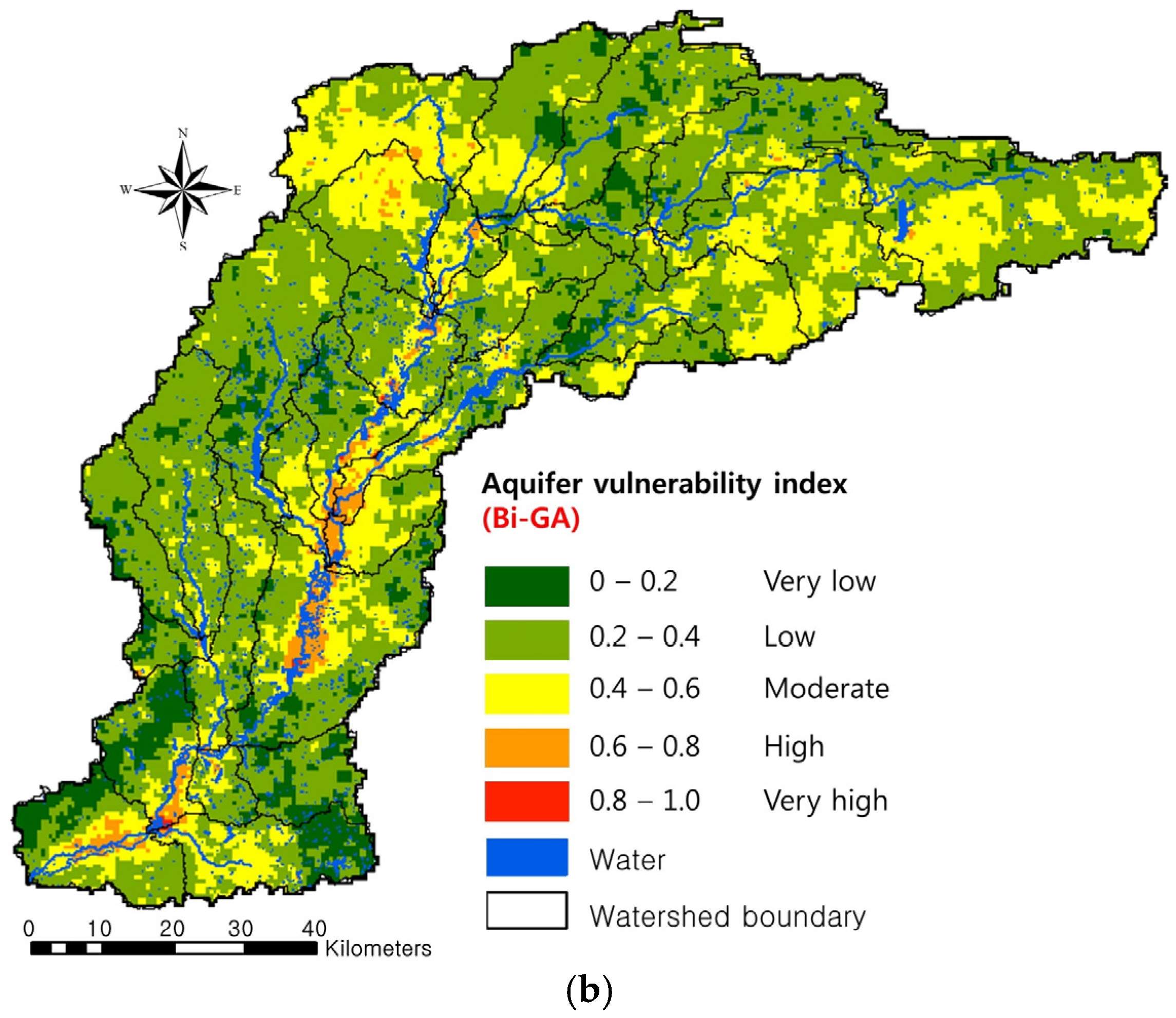
Figure 5.
Hotspot analysis maps to determine the potential groundwater monitoring and management sites.
Figure 5.
Hotspot analysis maps to determine the potential groundwater monitoring and management sites.
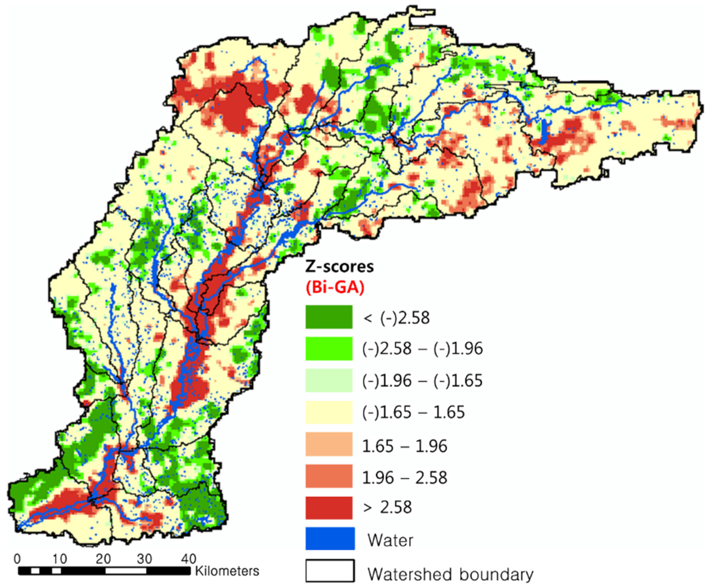
Table 1.
Data used for creating DRASTIC input data.
| Data Type | Source | Format | Scale | Date | Used to Produce |
|---|---|---|---|---|---|
| Water well | IDNR 1 | Point Shapefile | 1:24,000 | 1959–2010 | Depth to water |
| Annual Precipitation | NCDC 2 | Tabular data | - | 1949–2013 | Recharge |
| LULC | MRLC 3 | Raster | 1:250,000 | 2006 | Recharge |
| Aquifer Systems | USGS 4 | Polygon Shapefile Text | 1:48,000 | 2003–2011 | Aquifer media |
| SSURGO 5 | NRCS 6 | Polygon Shapefile | 1:12,000 | 2005 | Recharge Soil media Topography |
| iLITH data | IGS 7 | Point Shapefile | 1:24,000 | 2001 | Impact of vadose |
| Aquifer Transmissivity | IDNR 1 | Point Shapefile | 1:24,000 | 2011 | Conductivity |
1 IDNR: Indiana Department of Natural Resources; 2 NCDC: National Climate Data Center; 3 MRLC: Multi-Resolution Land Characteristics Consortium; 4 USGS: U.S. Geological Survey; 5 SSURGO: Soil Survey Geographic Database; 6 NRCS: Natural Resources Conservation Service; 7 IGS: Indiana Geological Survey.
Table 2.
Description of DRASTIC parameters and DRASTIC original weights.
| DRASTIC Parameters | Description | Original Weight |
|---|---|---|
| Depth to water (D) | Depth from the ground surface to the water table. Deeper water table levels imply lesser contamination chances. | 5 |
| Recharge (R) | Amount of water entering the aquifer. The amount of recharge is positively correlated with the vulnerability rating. | 4 |
| Aquifer media (A) | Material property of the saturated zone, which controls pollutant attenuation processes based on the permeability of each layer of media. | 3 |
| Soil media (S) | Soil media affects contaminant transport and water from soil surface to the aquifer. | 2 |
| Topography (T) | Slope of the land surface. For low slope, contaminant is less likely to become runoff and more likely to infiltrate. | 1 |
| Impact of vadose zone media (I) | Vadose zone is the typical soil horizon above the water table and below the ground surface. If vadose zone is highly permeable, this will lead to a high vulnerability rating. | 5 |
| Hydraulic conductivity (C) | Hydraulic conductivity represents the ability of the aquifer to transmit water. Hydraulic conductivity is positively correlated with the vulnerability rating. | 3 |
Table 3.
Typical and modified ranges and ratings of aquifer media (A).
| Aquifer Media | |||
|---|---|---|---|
| Range | Rating (Typical) | Vulnerability (IDNR Report) | Rating (Modified) |
| Karst limestone | 10 | Very high | 10 |
| Basalt | 9 | High | 8 |
| Sand and gravel | 8 | Moderate | 6 |
| Massive sandstone Massive limestone | 7 | Low | 4 |
| Bedded sandstone Limestone Shale | 6 | Very Low | 2 |
| Glacial till | 5 | ||
| Weathered metamorphic | 4 | ||
| Metamorphic Igneous | 3 | ||
| Massive shale | 2 | ||
Table 4.
Driving variables in Genetic Algorithm (GA) for DRASTIC parameter optimization.
| GA Driving Variables | Values |
|---|---|
| Population size | 100 |
| Max generation | 10,000 |
| Initial random value | 1000 |
| Min. value of parameters | 0 |
| Max. value of parameters | 6 |
| Crossover probability | 0.5 |
| Mutation probability | 0.02 |
Table 5.
Calibrated DRASTIC weights using Bi-GA for better prediction of aquifer vulnerability.
| Calibration Methods | D | R | A | S | T | I | C | RMSE |
|---|---|---|---|---|---|---|---|---|
| No calibration | 5 | 4 | 3 | 2 | 1 | 5 | 3 | 0.70 |
| Bi-GA 1 | 5.7 | 4.3 | 3 | 1.6 | 0.7 | 5.4 | 2.8 | 0.57 |
1 Bi-GA: Binary classifier calibration with genetic algorithm.
Table 6.
Error matrix to validate uncalibrated and calibrated DRASTIC.
| Uncalibrated DRASTIC | Calibrated DRASTIC | |||
|---|---|---|---|---|
| Reference Data | Reference Data | |||
| Classification | >2 ppm | >2 ppm | ||
| Very high + high 1 (>2 ppm) | 12 | Very high + high 1 (>2 ppm) | 16 | |
| Others 2 (≤2 ppm) | 23 | Others 2 (≤2 ppm) | 19 | |
1 Very high + high vulnerability areas; 2 Moderate + low + very low vulnerability areas.
Table 7.
Vulnerability areas (%) and number of nitrate detections >2 ppm without calibration.
| Class | Area (%) | Number of Nitrate Detections >2 ppm |
|---|---|---|
| Very low | 10.6 | 1 (0.9%) |
| Low | 60.4 | 4 (3.4%) |
| Moderate | 25.8 | 70 (60.3%) |
| High | 3.0 | 34 (29.3%) |
| Very high | 0.2 | 7 (6%) |
Table 8.
Vulnerability areas (%) and number of nitrate detections >2 ppm with calibration.
| Class | Area (%) | Number of Nitrate Detections >2 ppm |
|---|---|---|
| Very low | 9.6 | 0 (0%) |
| Low | 60.1 | 5 (4.3%) |
| Moderate | 26.9 | 62 (53.4%) |
| High | 3.2 | 42 (36.2%) |
| Very high | 0.2 | 7 (6%) |
Table 9.
Comparison of detection ratio between previous and current study.
| Navulur (1996) | ||||
|---|---|---|---|---|
| DRASTIC | SEEPAGE | Combined DL 1 | DRASTIC 2 | |
| HV-Area 3 (%) | 24.8 | 28.6 | 56.9 | 3.4 |
| N-Detections 4 (%) | 80.7 | 60.5 | 91.8 | 42.2 |
| Detection Ratio | 3.3 | 2.1 | 1.6 | 12.4 |
1 Combined DRASTIC and NLEAP; 2 Results from this study; 3 “High” and “Very high” vulnerability areas; 4 Percentage of nitrate detections.
Table 10.
Results of hotspot analysis using Gi* statistic method.
| Calibration Methods | Potential Groundwater Monitoring and Management Sites (%) | ||
|---|---|---|---|
| Z-Scores | |||
| 1.65–1.96 | 1.96–2.58 | >2.58 | |
| Bi-GA | 3.4 | 5.6 | 10.9 |
© 2017 by the authors. Licensee MDPI, Basel, Switzerland. This article is an open access article distributed under the terms and conditions of the Creative Commons Attribution (CC BY) license (http://creativecommons.org/licenses/by/4.0/).
Share and Cite
MDPI and ACS Style
Jang, W.S.; Engel, B.; Harbor, J.; Theller, L. Aquifer Vulnerability Assessment for Sustainable Groundwater Management Using DRASTIC. Water 2017, 9, 792. https://doi.org/10.3390/w9100792
AMA Style
Jang WS, Engel B, Harbor J, Theller L. Aquifer Vulnerability Assessment for Sustainable Groundwater Management Using DRASTIC. Water. 2017; 9(10):792. https://doi.org/10.3390/w9100792
Chicago/Turabian StyleJang, Won Seok, Bernard Engel, Jon Harbor, and Larry Theller. 2017. "Aquifer Vulnerability Assessment for Sustainable Groundwater Management Using DRASTIC" Water 9, no. 10: 792. https://doi.org/10.3390/w9100792
Note that from the first issue of 2016, this journal uses article numbers instead of page numbers. See further details here.