Hydrological Appraisal of Climate Change Impacts on the Water Resources of the Xijiang Basin, South China


1
School of Hydrometeorology, Nanjing University of Information Science and Technology, Nanjing 210044, China
2
Technology Centre, Hydraulic and Hydropower Project, Guangdong Province, Guangzhou 510635, China
*
Author to whom correspondence should be addressed.
Water 2017, 9(10), 793; https://doi.org/10.3390/w9100793
Submission received: 17 August 2017
/
Revised: 27 September 2017
/
Accepted: 11 October 2017
/
Published: 16 October 2017
Abstract
:Assessing the impact of climate change on streamflow is critical to understanding the changes to water resources and to improve water resource management. The use of hydrological models is a common practice to quantify and assess water resources in such situations. In this study, two hydrological models with different structures, e.g., a physically-based distributed model Liuxihe (LXH) and a lumped conceptual model Xinanjiang (XAJ) are employed to simulate the daily runoff in the Xijiang basin in South China, under historical (1964–2013) and future (2014–2099) climate conditions. The future climate series are downscaled from a global climate model (Beijing Climate Centre-Climate System Model, BCC-CSM version 1.1) by a high-resolution regional climate model under two representative concentration pathways—RCP4.5 and RCP8.5. The hydrological responses to climate change via the two rainfall–runoff models with different mathematical structures are compared, in relation to the uncertainties in hydrology and meteorology. It is found that the two rainfall–runoff models successfully simulate the historical runoff for the Xijiang basin, with a daily runoff Nash–Sutcliffe Efficiency of 0.80 for the LXH model and 0.89 for the XAJ model. The characteristics of high flow in the future are also analysed including their frequency (magnitude–return-period relationship). It shows that the distributed model could produce more streamflow and peak flow than the lumped model under the climate change scenarios. However the difference of the impact from the two climate scenarios is marginal on median monthly streamflow. The flood frequency analysis under climate change suggests that flood magnitudes in the future will be more severe than the historical floods with the same return period. Overall, the study reveals how uncertain it can be to quantify water resources with two different but well calibrated hydrological models.
1. Introduction
Climate change is expected to cause a significant variation of hydrological and water cycle systems by altering the radiative balance of the atmosphere, which may consequently result in changes of climatic variables, such as pressure, temperature, precipitation and others [1]. For regional water management, the influence of climate change on water resources and hydrological systems can be reflected both on the contents and approaches, such as the intensity and patterns of extreme rainfall events, the magnitude and frequency of extreme floods and droughts, the quality and quantity of local water availability and the vulnerability and management of water resource systems. Although not all of these impacts are necessarily negative, it is be crucial for local stakeholders and management committees to evaluate them as early as possible to understand how global climate change in the future could affect regional water supplies, because of the great socio-economic importance of water and other natural resources [2].
Global climate models (GCMs) are one of the primary tools to obtain present climate and projections of future global climate change using various greenhouse gas emission scenarios. Therefore, the following three procedures are suggested to study climate change impacts on hydrology and water resources: (1) use of GCMs to produce future global climate scenarios with different emission scenarios, (2) use of downscaling techniques to match GCM output with the scales compatible with hydrological models, and (3) use of hydrological modelling systems to simulate and analyse the effects of future climate change in the study area at various scales [3].
However, using hydrologic modelling systems to study global climate change impacts still involves two challenges: (1) scale differences between GCMs and hydrological models, (2) the different response of hydrological systems due to different hydrologic model structures and catchment characteristics. It was pointed out that the GCMs cannot represent the features and dynamics at the local subgrid-scale as significantly as at the continental scale [4,5]. Although statistical downscaling and dynamic downscaling techniques have been developed and widely applied in regional climate models (RCMs) to transform and obtain finer resolutions of GCM data, the application of regional hydrology and water resource studies using GCM/RCM data at the sub-grid scale is yet difficult [6,7]. Since the GCMs accuracy decreases when the spatial and temporal resolution becomes finer and the skill drops for surface variables such as precipitation, evapotranspiration and soil moisture, all of which are key elements for hydrological models [3]. Thus more uncertainties are expected for the projected future change of precipitation sums, intensities and patterns using downscaling techniques [6,8,9]. Therefore, the number of studies focusing on regional hydrological impact assessments of climate change is relatively small, in contrast to a large number of GCM downscaling studies [10].
In terms of the different response of hydrological systems, the range of diversity of regional hydrological responses under climate change scenarios, due to different hydrological model structures, has not been widely investigated and reported in the literature. Clark et al. (2008) [11] proposed a methodology to diagnose differences in 79 hydrological model structures by combining components of four hydrological models. Although the results suggested that the choice of model structure is just as important as the choice of model parameters, further study is still required to evaluate the model structural differences in various climate regimes. Boorman and Sefton (1997) [12] investigated the range of uncertainties resulting from two climate scenarios and eight climate sensitivity tests that were applied to three catchments using two conceptual hydrological models in the UK. It was concluded that the variation of the climate change impact on flow can be significant between catchments, and the different flow response indices can change in opposite directions even for the same climate scenario. The study also suggested that more studies should be conducted to compare the impacts due to different hydrological models, which would help to quantify the uncertainties resulting from the different model strictures and parameters.
Panagoulia and Dimou (1997a, b) [13,14] examined and compared the differences of two hydrological models under historical and future climate conditions. It was shown that the model’s sensitivity to greater temperature and precipitation varies in different climates. Jiang et al. (2007) [2] utilised six-monthly water balance models from the Dongjiang basin, China to assess uncertainty in hydrological responses to the climatic scenarios resulting from the use of different hydrological models. The results indicated that the climate change impacts on hydrological systems vary and depend on the hydrological model structures, even under the same future climate scenarios. Li et al. (2014) [15] used two rainfall–runoff models, Hydrologic Simulation Model (SIMHYD) and GR4J to simulate the monthly and annual runoff in the upstream catchments of the Yarlung Tsangpo River basin (YTR). The two rainfall–runoff models successfully simulate the historical runoff and show similar simulation results for the eight catchments in the YTR basins. Fischer et al. (2013) [16] used the standardized precipitation index (SPI-24) and the standardized discharge index (SDI-24) were used to analysis the hydrological long-term dry and wet sequences on the Xijiang River without using any hydrological models.
The studies reported in the literature and discussed above have only used two or more lumped hydrological models to simulate the impact of postulated climate changes and then analyse the hydrological responses from different hydrological models, which however only represent the results of the lumped hydrological models. It is therefore desirable to compare the differences in hydrological impact of alternative climates resulting from the use of physically-based distributed hydrological models, because the spatially explicit data of elevation, land use cover, and soil properties can not only represent the catchment characteristics and reflect on the parameterisation [17], but also take full advantage of gridded GCM/RCM output to predict hydrological responses to various climate scenarios [18].
In this study, a physically-based distributed model Liuxihe (LXH) and a conceptual lumped model Xinanjiang (XAJ) are used and their capabilities in reproducing historical water balance components and in predicting the hydrological impacts of alternative climates are compared. The main objective of this study is to show how uncertain it could be to quantify and assess water resources with two different but well-calibrated models under climate change. In this context, the study is focused on quantifying how large a difference one can expect when using lumped and distributed hydrological models to simulate the impact of climate change as compared to the model capabilities in simulating historical river flow discharges. The study is performed in two steps: first, the performance of models in reproducing historical streamflow components is evaluated; and second, the differences in the simulated hydrological flows under climate change by the lumped and distributed models are evaluated and compared.
2. Data and Methodology
2.1. Methodology
In this study, a physically-based distributed model, LXH, and a conceptual lumped model, XAJ, were constructed on the Xijiang Basin located in South China. The parameters for each model were calibrated and validated with historical observation data. The trial-and-error method based on the results of model parameter sensitivity analysis using global extend FAST (Fourier Amplitude Sensitivity Test) method was employed for the LXH model parameter calibration, whereas, the shuffle complex evolution algorithm developed at the University of Arizona (SCE-UA) [19] was used to optimize the parameters for the XAJ lumped model. Once calibrated, the two models were fed with the RCM historical simulations to verify the reliability of the climate data against the observations. Subsequently, two hydrological models were driven by the RCM with two emission scenarios (RCP4.5 and RCP8.5) to produce multiple runoff simulations. The RCM-based daily climate simulations were expected to capture the changes in daily climate variables that directly related to the analysis of extreme events relating to daily precipitation intensity and flood frequency.
2.2. Study Area and Hydrological Data
The study area is the Xijiang (West River) basin, a tributary of the Pearl River in southern China. The main Xijiang basin is a coastal area, located in the Guangxi province in South China. It has a sub-tropical monsoon climate, characterized by large interannual variability of precipitation and widely distributed floods with high frequency, which result in massive damage to property and life.
The average annual runoff recorded at the Wuzhou flow station is 224 billion cubic meters, accounting for 81.4% of the total runoff in Guangxi province. Thus the hydrological data of Wuzhou station is capable of reflecting the occurrence and the magnitude of floods in the Xijiang basin. Due to the data availability and reliability, the considered hydrological models were constructed on the Xijiang basin using the Wuzhou flow station as the catchment outlet. Therefore the whole drainage area is the upstream area above Wuzhou station, which is around 337,000 km2.
Although the Xijing basin is characterized by construction, like many other large rivers in China, the influence of the construction of reservoirs/dams on annual water discharge is much lower than the variability in precipitation [20], especially as the regulation of hydraulic structures on the main stream are usually on an hourly basis instead of daily, which has less influence on daily/monthly streamflow simulations.
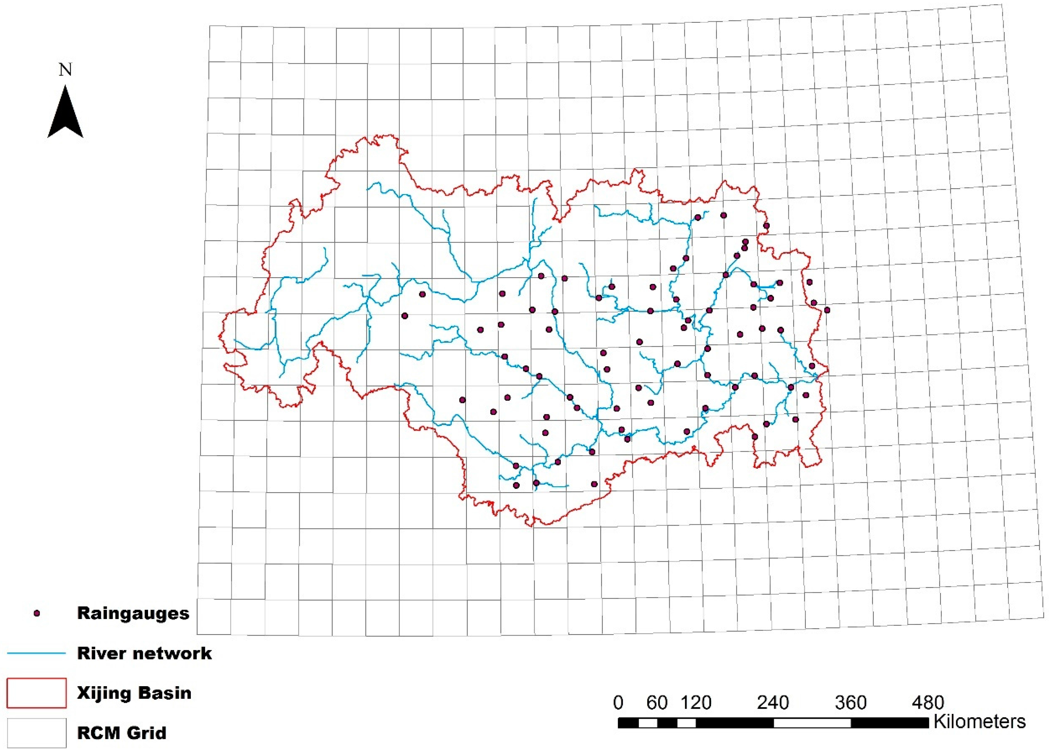
The data for model calibration and validation include observed daily evaporation, rainfall and streamflow data. All the data were obtained from the published Yearly Hydrological Books of China for the period from 1960 to 2006. In this study, the 74 major stations shown in Figure 1, which are almost evenly distributed over the whole basin, with 60 years of continuous records (1960–1988), were selected for model calibration (1 January 1973 to 1 January 1978) and validation (1 January 1979 to 31 December 1984 and 1 January 2006/1/1 to 31 December 2013).
2.3. Climate Change Scenarios and Datasets
The climate data used in this study are driven by the GCM, Beijing Climate Centre Climate System Model version 1.1 (BCC_CSM1.1). The projection of the climate change data on the Xijiang basin is simulated by a regional climate model (RegCM4.0) under two emission scenarios of the representative concentration pathways—RCP4.5 and RCP8.5. This is based on a period of transient simulations from 1950 to 2099, with a 0.5° horizontal resolution [21].
The outputs of RegCM4.0 consists of historical, RCP4.5, and RCP8.5 datasets, and each dataset provides projected mean temperature, maximum temperature, minimum temperature and precipitation on a daily basis. The representative concentration pathways (RCPs) are used for climate modelling and research, which describe four possible climate future scenarios depending on how much radiative gas is emitted in the future. The RCP4.5 is the intermediate emissions scenario in which the radiative force is stabilised at 4.5 W/m2 by 2100 without overshoot. The RCP8.5 is the high emissions scenario in which the radiative force rises to 8.5 W/m2 by 2100 [22]. For the projection of climate change, the difference between the 2006–2099 period in the RCP4.5 and RCP8.5 experiment, and the 1961–2005 period in the historical experiment, will be analysed in this study.
3. Hydrological Modelling and Parametrisation
3.1. Lumped Xinanjiang Model (XAJ)
The Xinanjiang model (XAJ) is a rainfall–runoff watershed model for use in humid and semi-humid regions, developed in 1973 in China [23]. XAJ has been widely used in China since 1980, mainly for flood simulation and forecasting. The model assumes that runoff production occurs on the repletion of storage to capacity values, which are assumed to be distributed throughout the basin. The runoff is divided into three components, including surface runoff, interflow and groundwater. The basin is divided into a set of sub-basins, the outflow hydrograph from each sub-basin is first simulated and then routed down the channels to the basin outlet. The flow chart of XAJ is shown in Figure 2.
3.2. Distributed Liuxihe Model (LXH)
The Liuxihe Model (LXH) is a physically-based, distributed hydrological model for river basin flood forecasting/simulation [24]. The LXH consists of several submodels, including the basin digitization model (BDM), the evapotranspiration model (EM), the runoff production model (RPM), the runoff routing model (RRM), and the parameter deriving model (PDM). The LXH model divides the catchment into a number of gridded cells, and each cell consists of three layers vertically, representing the surface, unsaturated and saturated zones. The EM module is then used to calculate the evapotranspiration for each cell. The RPM and RRM modules calculate the runoff produced for each cell and route runoff to the catchment outlet, respectively. The PDM module is responsible for model parameterisation. The detailed model structures are shown in Figure 3.
The DEM used in this study is derived from the 1’’ × 1’’ resolution shuttle radar topography mission (SRTM) data, provided by the Chinese Geospatial Data Cloud (http://www.gscloud.cn). The Xijiang Basin is a mountainous area, with a range of elevation from sea level to about 2830 m. The spatial resolution of raw DEM is about 90 m and was bilinear resampled to 500 m resolution for BDM in the LXH model.
The land use data was obtained from the 1km resolution of the global land cover database provided by the Global Observatory of Maryland University and the Institute of Geographic Sciences and Natural Resources Research, Chinese Academy of Sciences. The data was resampled to 500 m resolution using the nearest neighbour algorithm. There are 12 types of land use in Xijiang Basin, including water body, evergreen coniferous forest, evergreen broad-leaved forest, deciduous broad-leaved forest, mixed forest, forested grassland, closed shrub, open shrub, and grassland, which accounting for 0.390%, 1.617%, 0.939%, 0.326%, 0.001%, 7.407%, 25.351%, 0.133%, 0.001%, 22.507%, 41.295% and 0.034%, respectively. This suggests that the cultivated land is the main land use type, accounting for 41.295% of area in Xijiang Basin.
The soil properties used in this study were obtained from the Nanjing Soil Institute of the Chinese Academy of Sciences. There are seven types of soils in Xijiang Basin, including clay, silty loam, loam, sandy, loam, sandy loam and sand, which account for 57.94%, 4.20%, 22.56%, 14.90%, 0.05%, respectively. It is clear that clay accounts for more than half of the catchment area. The soil property parameters, such as soil thickness, water content at saturated condition, field capacity, wilting point, infiltration rate and hydraulic conductivity, were calculated by the soil water characteristics hydraulic properties calculator.
3.3. Model Calibration and Validation
Considering the data consistency and reliability due to the relocation of the Wuzhou flow station, the observed daily hydrological data selected for the model calibration was from 1 January 1973 to 1 January 1978, and the model validations were from 1 January 1979 to 31 December 1984 and 1 January 2006 to 31 December 2013. In order to evaluate the performance of the modelling results, it is a common practice to employ some criteria for judging model performance. Five different criteria, including the Nash–Sutcliffe efficiency coefficient (NS), correlation coefficient (Cor), root mean square error (RMSE), total water balance error coefficient (Dv) and average logarithm mean square error (MSLE), were used for different assessment purposes. The M and Q represent the simulated and observed flow respectively in the equations below:
The Nash–Sutcliffe efficiency coefficient (NS) is one of the most popular evaluation criteria for hydrological modelling to measure the degree of association between observed and simulated values:
The correlation coefficient (Cor) is the linear correlation to describe the discrete degree between the observation and the simulation. The closer to one, the more correlated it is.
Root mean square error (RMSE) is used to evaluate the total water error, which is simply the average of the squared errors for all the simulation results, providing an objective measure of the difference between the observed and simulated values:
The total peak flow error (PF) is the ratio of total peak flow runoff error to observed peak flow runoff. The M and Q in this equation represent the sum of peak flows in each year during the simulation period:
The mean square logarithm error (MSLE) is high in low-flow error and small in peak-flow error, which can be used to estimate the total water error, but more to focus on low-flow and base-flow components:
The statistics for the two models for the calibration and validation periods are listed in Table 1. It suggests that the distributed LXH model and lumped XAJ model have better performance on calibration (1 January 1973 to 1 January 1978) and validation one period (1 January 1979 to 31 December 1984) than the validation two period (1 January 2006 to 31 December 2013). Since the simulated peak flows from both models in the validation two period, especially the small and medium size peak flows are much less present in the observations. It may imply that the difference reflects the influence of human activities on the hydrological processes in the past 30 years, since the 1980s. Since a large number of water conservancy projects, water storage, and water diversion projects may have changed the natural runoff conditions in the Xijiang basin, part of the small- and medium-sized peak flows were actually blocked by water conservancy projects, which is why it was not consistent with the model simulations.
Although the NS and Cor criteria indicate that both the LXH and XAJ models show relatively good performance for the Xijing basin simulation, the MSLE suggests that the XAJ model outperformed the LXH model in the base flow simulation, but the LXH model is more accurate than XAJ in the peak flow simulations according to the PF statistic. However, considering the computational cost and the parametrisation process, the lumped XAJ model is much more cost-effective than the distributed LXH model.
4. Results and Discussion
The reliability and accuracy of historical precipitation data produced from the climate models (RF) was first evaluated against the observed rainfall data through the two hydrological models during validation period one, in order to examine the data reliability and accuracy produced by the climate model. Then the rainfall data under the RCP4.5 and RCP8.5 scenarios obtained from the climate models were assessed against the observation data through the two hydrological models during validation period two. Finally, the projected rainfall data under the RCP4.5 and RCP8.5 scenarios from 2006 to 2099 were used as the input in the two hydrological models and the related flood frequency analysis was carried out.
4.1. Evaluation of Rainfall Products from the Climate Model
According to the availability of the climate rainfall data and observation flow data, the historical rainfall climate data was assessed against the rain gauge measurements through the two hydrological models during the model validation period one (1 January 1979 to 31 December 1984). The position of the RCM grids and catchment boundaries are illustrated in Figure 4, which displays how the RCM data are used to feed the distributed LXH model, while the RCM data were averaged to the catchment mean value to feed the lumped XAJ model, according to the weighting of grid area on the catchment.
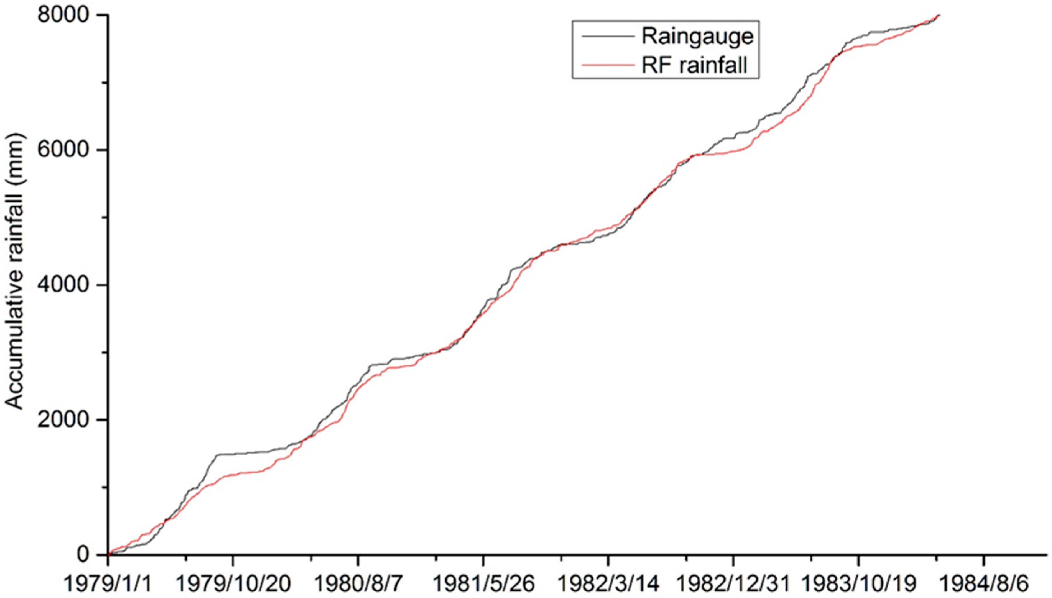
Figure 5 shows that the cumulative catchment rainfall derived from historical precipitation in the climate model has fairly good agreement with the cumulative rain gauge measurements over the Xijiang basin, with only a 2.43% difference in total cumulative rainfall. However, Figure 6 indicates that the scatter is relatively high and the RF data tend to underestimate, compared to the rain gauge measurements.
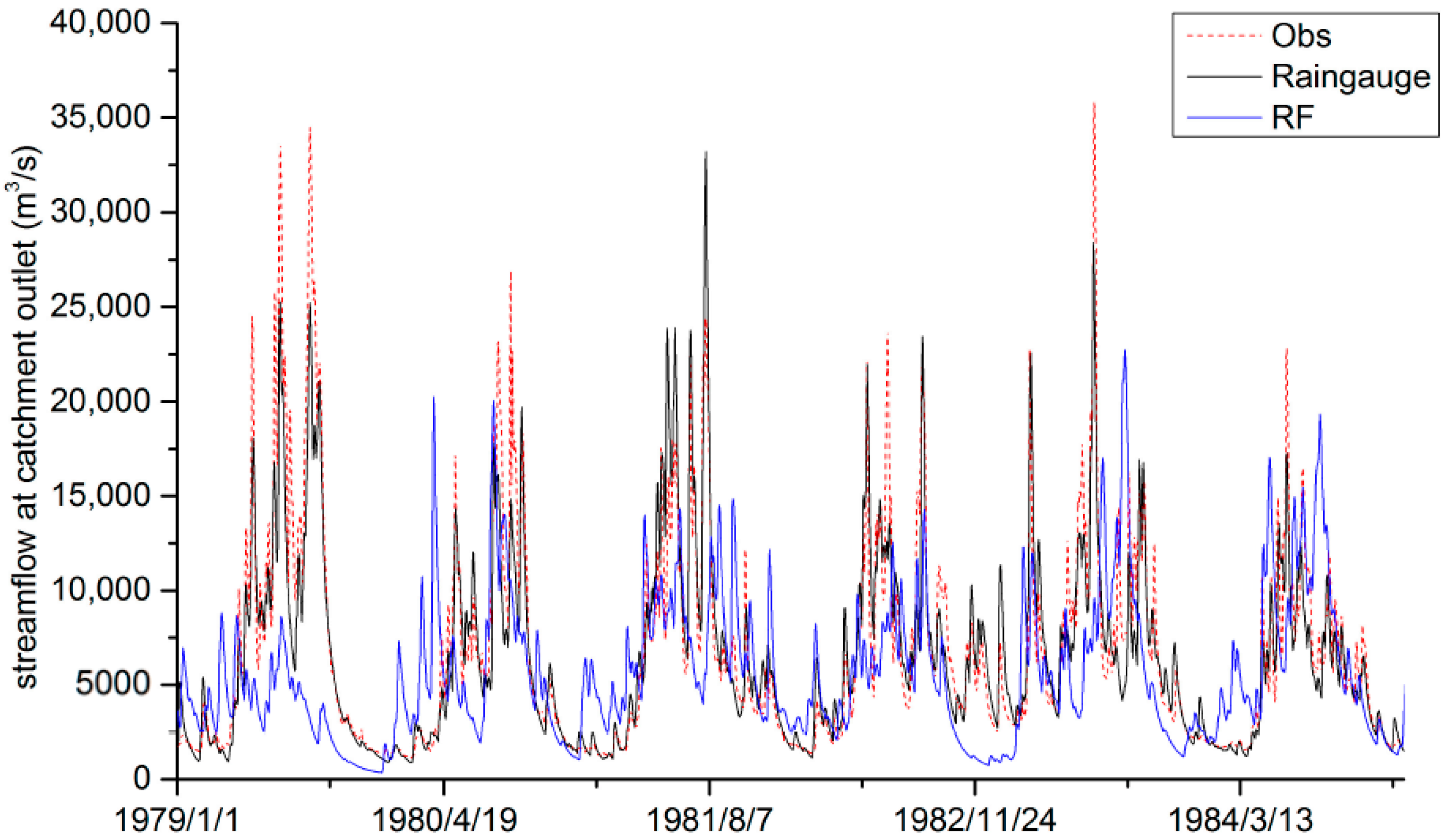
The NS statistic (0.45 in XAJ and 0.83 in LXH) suggested that the simulation results driven by the RF in the two models are slightly more accurate than the mean of the observed data, although the trend of the hydrographs agreed with the observations (see Figure 7 and Figure 8). Additionally, the streamflow simulations in the XAJ and LXH models driven by RF produced more peak flows but much less peak flow volume than the observation and the simulation using rain gauge measurements, especially in the XAJ model. Since the LXH model is fully distributed and supposed to represent the distribution of the gridded rainfall from the climate model better than the lumped XAJ model, it subsequently had better performance for peak flow simulations.
In summary, the historical precipitation data (RF) and RCP rainfall products from the climate model are consistent with rain gauge observations in terms of the pattern of the catchment rainfall accumulation curve and the total precipitation over the catchment. Also, the patterns of the hydrographs driven by the climate models generated rainfall data in two hydrological models that are quite similar to the observation and the hydrographs driven by the rain gauges. Nevertheless, the climate model rainfall data tended to trigger more small and medium peak flows, but to underestimate the high peak flows during the two validation periods. It implies that the rainfall data from the climate model is possibly more reliable for use in monthly and annual water resource simulation and analysis.
4.2. Future Rainfall–Runoff Simulations
The projected rainfall data under the RCP4.5 and RCP8.5 scenarios from 2006 to 2099 were used as the input in the two hydrological models. However, the simulation results were averaged to the monthly and annual time scale for analysis.
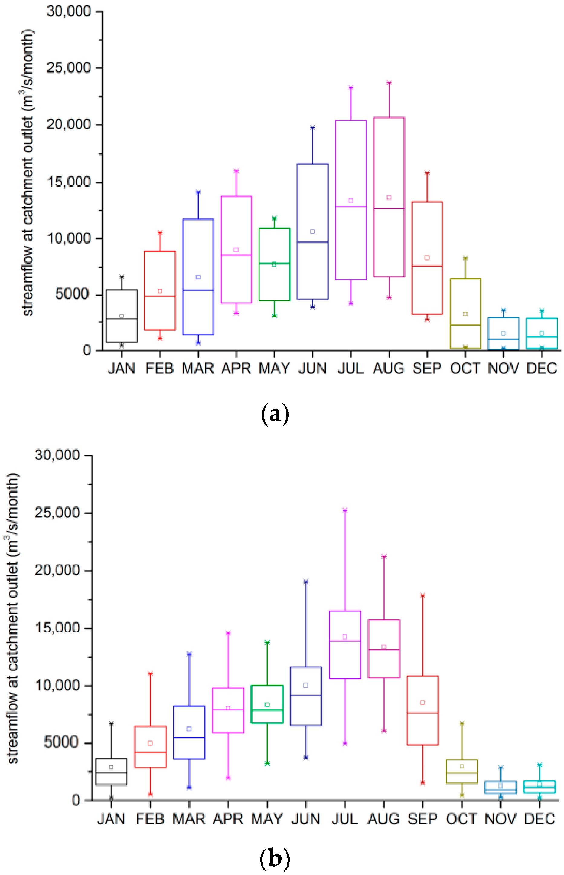
For the distributed LXH model, the modelled flow results are listed in Table 2 and the box plots are illustrated in Figure 9. Both the RCP4.5 and RCP8.5 scenario suggests that the highest flow will occur in July, whereas the lowest flow is expected in November, according to the monthly flow median value, although the difference derived from the two scenarios is rather marginal. For the high flow in July, the average streamflow in the Xijiang basin under the RCP4.5 scenario is 12,850 m3/s, less than the flow modelled under RCP8.5, which is 13,916 m3/s, around 8.30% difference. For the low flow in November, the average streamflow in the Xijiang basin under the RCP4.5 scenario is 991 m3/s, higher than flow modelled under RCP8.5, which is 931 m3/s, around 6.05% difference.
Compared to the distributed LXH model, the simulation results achieved in the lumped XAJ model show the highest flow in the Xijiang basin will occur in August, whereas the lowest flow is expected in December, according to the mean monthly flow median value under the two RCP scenarios (see Figure 10).
Table 3 shows that the highest average streamflow in the Xijiang basin under the RCP4.5 scenario is 10,323 m3/s in August, less than 10,514 m3/s under RCP8.5, which is around 1.85% difference. During the dry season, the lowest mean monthly flow simulation found under the RCP4.5 scenario is 1451 m3/s, higher than the flow modelled under RCP8.5, which is 1422 m3/s, around 1.99% difference. Similar to the assessment in the LXH model, the two RCP scenarios produced much less variation in the average monthly flow in the Xijiang basin under climate change from 2006 to 2099.
Regarding the RCP rainfall performance in the two hydrological models, Figure 11 illustrates the comparisons of the median monthly flow simulation under two climate change scenarios in the LXH and XAJ models. It is clear to show that the distributed LXH model produced more streamflow than the lumped XAJ model during January to August, especially during the high rainfall rate seasons, but more streamflow was modelled in the XAJ model than the LXH model during September to December. Since the distributed model can reflect the spatial rainfall distribution better than the lumped model and thus has more influence on the peak flow volume, while the lumped XAJ model outperformed the LXH model on the base flow in this study, which was also due to the different rainfall–runoff mechanisms and mathematical structures of the two models.
In addition, the annual flow simulation shown in Figure 12 illustrates the variation between the two scenarios in the two hydrological models. It suggests that the RCP4.5 rainfall produced the smallest and the highest annual streamflow in the XAJ and LXH model, respectively, in the Xijiang basin before 2050. Nevertheless, the RCP8.5 rainfall produced the smallest annual streamflow in XAJ and the highest annual streamflow in the LXH model from 2050 to 2099. In general, for both RCP rainfall products, more annual streamflow is modelled in the LXH model than in the XAJ model.
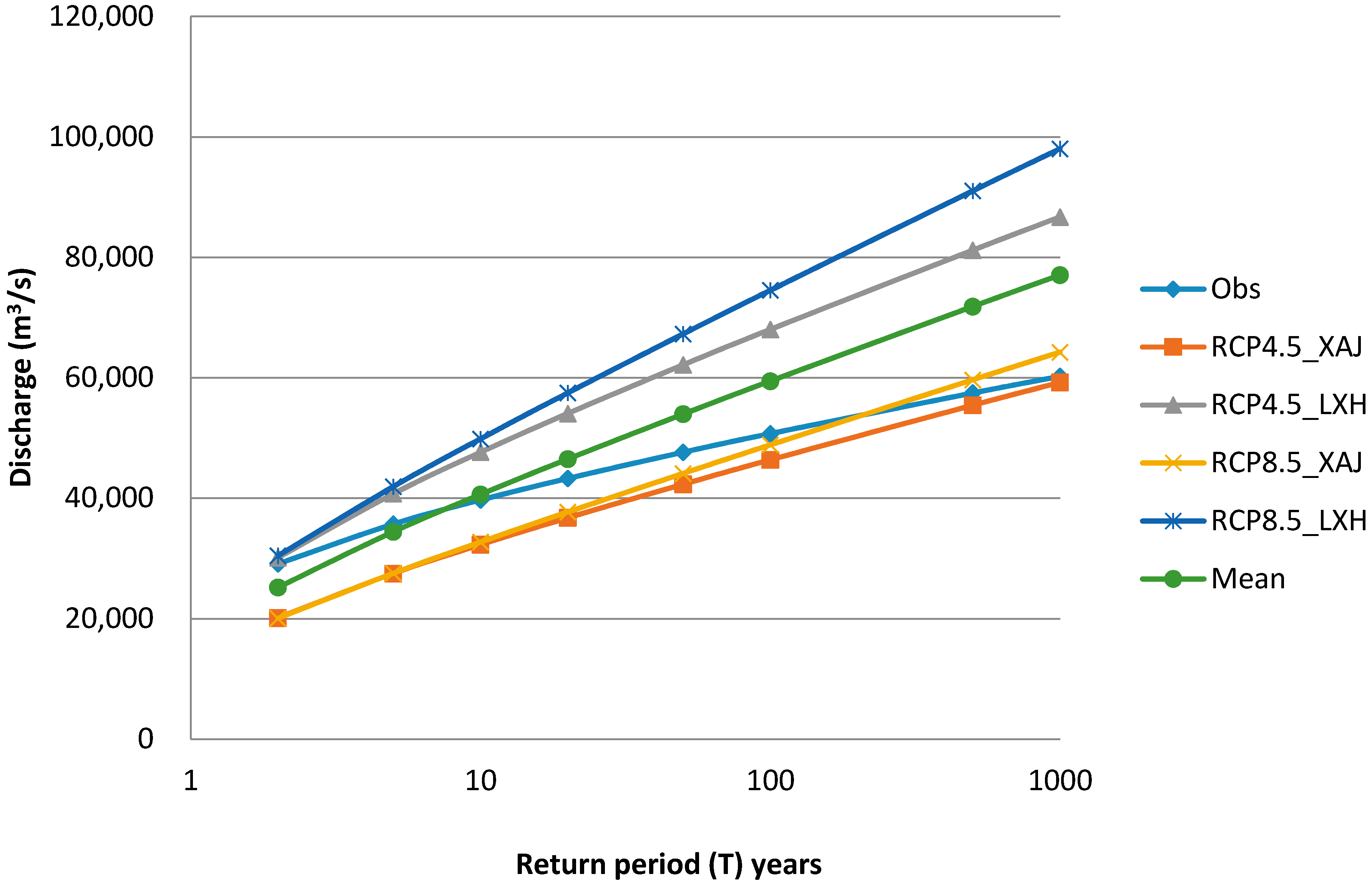
In order to analyse the flood magnitude under different scenarios in the future, this study used the Log–Pearson Type 3 (LP3) distribution to estimate flood magnitude under climate change, which is the recommended distribution for estimating return period values of flood magnitude in China [25]. The distribution has the following form with the data being preliminary log transformed [26]:
where is a location; is a shape; and is a scale parameter.
The method of L-moments was used to estimate the parameters of LP3 distribution in this study. L-moments are analogous to conventional moments defined as linear combinations of probability weighted moments (PWMs) [26]. The method is proven to be superior to other common parameter estimation techniques such as the maximum likelihood [27] and the method of moments [28].
The details of the parameter estimation procedure based on L-moments can be found in Hosking and Wallis (1997) [26] and Das (2016) [28]. The above LP3 flood frequency model was applied to the annual maximum (AM) flow series derived from the observed flow data and future flow series simulated using hydrological models based on future climate data.
The predicted return period flood magnitudes for different series are plotted in Figure 13, which indicate that the range of design values increase along with the return period. This also provides an uncertainty bound which can be expected in the future.
According to the lumped XAJ model simulation results, the future flood magnitude is similar to the historical floods, and the floods under the climate change scenarios with less than 100-year return periods are less severe than the historical floods, and the floods with a 1000-year return period are rather close to the historical records. However, the floods simulated under same future scenarios in the distributed LXH model are much more severe than the historical floods, especially under the RCP8.5 scenarios. Consequently, the mean flood magnitude in the future illustrated in Figure 13 indicates that the floods under climate change are likely to be more severe than the historical floods.
5. Summary and Concluding Comments
In this study, two hydrological models with different mathematical structures were used and their differences in reproducing historical streamflow and in predicting the hydrological impacts of two climate change scenarios (RCP4.5 and RCP8.5) were compared. The study was performed on the Xijiang catchment, a tributary of the Pearl River, located in a subtropical humid region in southern China. The main focus of the study was to test how uncertain one can expect the estimations to be when using fully-distributed and lumped rainfall–runoff models to simulate hydrological responses to climate changes, as compared to their capacities in simulating historical runoff. The following conclusions are drawn from the study:
- (1)
- Both the distributed LXH model and lumped XAJ models can reproduce almost equally well the historical runoff data series. The simulated peak flows were more accurate in the LXH model, while the base flow was better simulated by the XAJ model.
- (2)
- The cumulative catchment daily rainfall produced from the climate model matched the rain gauge measurements very well, but they tended to produce more small and medium peak flows and to underestimate the high peak flows during the hydrological model simulations.
- (3)
- Using RCP4.5 and RCP8.5 precipitation data as input to the tested models, marginal variations were found in the median flow simulation in the same hydrological model, which may imply that the difference of the impact from the two climate scenarios on the monthly streamflow simulation in this study was small.
- (4)
- Under future climate conditions, the distributed LXH model produced more streamflow than the lumped XAJ model during January to August, but more streamflow was modelled in the XAJ model than in the LXH model from September to December.
- (5)
- The RCP4.5 climate data could result in the smallest and the highest annual streamflow in the XAJ and LXH models respectively before 2050, but the RCP8.5 rainfall data could produce the smallest annual streamflow in the XAJ and the highest annual streamflow in the LXH model from 2050 to 2099.
- (6)
- The flood frequency analysis suggests that the floods under climate change in the future will be more severe than the historical floods, especially under the RCP8.5 scenario in the LXH model simulations.
This study shows that the difference in the streamflow simulations depend on the climate scenarios, the season, and the hydrological model structures that span from complex to simple, reflecting a decreasing ability to specifically represent the distributed (spatial) nature of the rainfall–runoff process. In this study, the exanimated distributed model could produce more streamflow and peak flow than the lumped model under the climate change scenarios, but the lumped model outperformed in the base flow simulation. This suggests that attention must be paid when using the hydrological models to simulate hydrological responses under climate change. Comparing the median monthly modelled flow driven by the RCP4.5 and RCP8.5 scenarios, the RCP4.5 data could produce more flow during the dry season while the RCP8.5 data could trigger higher flow in the flood season.
The approach of using different hydrological models with different climate scenarios could also be appropriate for the uncertainty analysis of monthly, seasonal and annual scale runoff changes. It is noted that this study does not consider the uncertainty of hydrological model parameters. Future water resource scenarios predicted by any particular hydrological model represent only the results specific to that model. More studies using different hydrological models for different catchments need to be carried out in order to provide more general conclusions.
Acknowledgments
The work presented in this paper was partly supported by the National Key Research and Development Program of China (No. 2016YFA0601703). We acknowledge the modelling groups for providing their data for analysis, the Program for Climate Model Diagnosis and Intercomparison (PCMDI) and the World Climate Research Programme’s (WCRP’s) Coupled Model Intercomparison Project for collecting and archiving the model output, and organizing the model data analysis activity. The regional climate model data was collected, analysed, and provided by the National Climate Centre.
Author Contributions
Dehua Zhu designed research and wrote the paper. Qiwei Ren conducted data analysis and Samiran Das contributed to the discussion and writing part of the paper.
Conflicts of Interest
The authors declare no conflict of interest.
References
- Houghton, J.T.; Jenkins, G.J.; Ephraums, J.J. (Eds.) Climate Change. The IPCC Assessment; Cambridge University Press: New York, NY, USA, 1990. [Google Scholar]
- Jiang, T.; Chen, Y.D.; Xu, C.Y.; Chen, X.; Chen, X.; Singh, V.P. Comparison of hydrological impacts of climate change simulated by six hydrological models in the Dongjiang Basin, South China. J. Hydrol. 2007, 336, 316–333. [Google Scholar] [CrossRef]
- Xu, C.Y.; Widén, E.; Halldin, S. Modelling hydrological consequences of climate change-progress and challenges. Adv. Atmos. Sci. 2005, 22, 789–797. [Google Scholar] [CrossRef]
- Wigley, T.M.L.; Jones, P.D.; Briffa, K.R.; Smith, G. Obtaining sub-gridscale information from coarse-resolution general circulation model output. J. Geophys. Res. 1990, 95, 1943–1953. [Google Scholar] [CrossRef]
- Carter, T.R.; Parry, M.L.; Harasawa, H.; Nishioka, S. IPCC Technical Guidelines for Assessing Climate Change Impacts and Adaptions; IPCC Special Report to Working Group II of IPCC; Department of Geography, University College London: London, UK, 1994. [Google Scholar]
- Fowler, H.J.; Blenkinsop, S.; Tebaldi, C. Review Linking climate change modelling to impacts studies: Recent advances in downscaling techniques for hydrological modelling. Int. J. Climatol. 2007, 27, 1547–1578. [Google Scholar] [CrossRef]
- Wang, D.; Hagen, S.C.; Alizad, K. Climate change impact and uncertainty analysis of extreme rainfall events in the Apalachicola River basin, Florida. J. Hydrol. 2013, 480, 125–135. [Google Scholar] [CrossRef]
- Wood, A.W.; Leung, L.R.; Sridhar, V.; Lettenmaier, D.P. Hydrologic implications of dynamical and statistical approaches to downscaling climate model outputs. Clim. Chang. 2004, 62, 189–216. [Google Scholar] [CrossRef]
- Immerzeel, W.W.; Droogers, P.; de Jong, S.M.; Bierkens, M.F.P. Large-scale monitoring of snow cover and runoff simulation in Himalayan river basins using remote sensing. Remote Sens. Environ. 2009, 113, 40–49. [Google Scholar] [CrossRef]
- Raposo, J.R.; Dafonte, J.; Molinero, J. Assessing the impact of future climate change on groundwater recharge in Galicia-Costa, Spain. J. Hydrol. 2013, 21, 459–479. [Google Scholar] [CrossRef]
- Clark, M.P.; Slater, A.G.; Rupp, D.E.; Woods, R.A.; Vrugt, J.A.; Gupta, H.V.; Wagener, T.; Hay, L.E. Framework for Understanding Structural Errors (FUSE): A modular framework to diagnose differences between hydrological models. Water Resour. Res. 2008, 44, W00B02. [Google Scholar] [CrossRef]
- Boorman, D.B.; Sefton, C.E.M. Recognising the uncertainty in the quantification of the effects of climate change on hydrological response. Clim. Chang. 1997, 35, 415–434. [Google Scholar] [CrossRef]
- Panagoulia, D.; Dimou, G. Linking space-time scale in hydrological modelling with respect to global climate change. Part 1. Models, model properties, and experimental design. J. Hydrol. 1997, 194, 15–37. [Google Scholar] [CrossRef]
- Panagoulia, D.; Dimou, G. Linking space-time scale in hydrological modelling with respect to global climate change. Part 2. Hydrological response for alternative climates. J. Hydrol. 1997, 194, 38–63. [Google Scholar] [CrossRef]
- Li, F.; Xu, Z.; Liu, W.; Zhang, Y. The impact of climate change on runoff in the Yarlung Tsangpo River basin in the Tibetan Plateau. Stoch. Environ. Res. Risk Assess. 2014, 28, 517–526. [Google Scholar] [CrossRef]
- Fischer, T.; Gemmer, M.; Su, B.; Scholten, T. Hydrological long-term dry and wet periods in the Xijiang river basin, south china. Hydrol. Earth Syst. Sci. 2013, 17, 135–148. [Google Scholar] [CrossRef] [Green Version]
- Gotzinger, J.; Bardossy, A. Generic error model for calibration and uncertainty estimation of hydrological models. Water Resour. Res. 2008, 44, 35. [Google Scholar] [CrossRef]
- Browning, D.M.; Duniway, M.C. Digital soil mapping in the absence of field training data: A case study using terrain attributes and semiautomated soil signature derivation to distinguish ecological potential. Appl. Environ. Soil Sci. 2011, 2011, 421904. [Google Scholar] [CrossRef]
- Duan, Q.; Sorooshian, S.; Gupta, V.K. Effective and efficient global optimization for conceptual rainfall–runoff models. Water Resour. Res. 1992, 28, 1015–1031. [Google Scholar] [CrossRef]
- Zhang, S.; Lu, X.X.; Higgitt, D.L.; Chen, C.T.A.; Han, J.; Sun, H. Recent changes of water discharge and sediment load in the Zhujiang (Pearl River) Basin, China. Glob. Planet Chang. 2008, 60, 365–380. [Google Scholar] [CrossRef]
- Gao, X.J.; Wang, M.L.; Giorgi, F. Climate change over China in the 21st century as simulated by BCC_CSM1. 1-RegCM4.0. Atmos. Ocean. Sci. Lett. 2013, 6, 381–386. [Google Scholar]
- Van Vuuren, D.P.; Edmonds, J.; Kainuma, M.; Riahi, K.; Thomson, A.; Hibbard, K.; Hurtt, G.C.; Kram, T.; Krey, V.; Lamarque, J.F.; et al. The representative concentration pathways: An overview. Clim. Chang. 2011, 109, 5. [Google Scholar] [CrossRef]
- Zhao, R.J. The Xinanjiang model applied in China. J. Hydrol. 1992, 135, 371–381. [Google Scholar]
- Chen, Y.; Ren, Q.; Huang, F.; Xu, H.; Cluckie, I. Liuxihe Model and its modeling to river basin flood. J. Hydrol. Eng. 2010, 16, 33–50. [Google Scholar] [CrossRef]
- Fang, B.; Guo, S.; Wang, S.; Liu, P.; Xiao, Y. Non-identical models for seasonal flood frequency analysis. Hydrol. Sci. J. 2007, 52, 974–991. [Google Scholar] [CrossRef]
- Hosking, J.R.M.; Wallis, J.R. Regional Frequency Analysis: An Approach Based on L-Moments; Cambridge University Press: New York, NY, USA, 1997. [Google Scholar]
- Hosking, J.R. Algorithm as 215: Maximum-likelihood estimation of the parameters of the generalized extreme-value distribution. J. R. Stat. Soc. Ser. C Appl. Stat. 1985, 34, 301–310. [Google Scholar] [CrossRef]
- Das, S. An assessment of using subsampling method in selection of a flood frequency distribution. Stoch. Environ. Res. Risk Assess. 2016, 1–13. [Google Scholar] [CrossRef]
Figure 1.
Xijiang Basin (upstream of Wuzhou flow station).
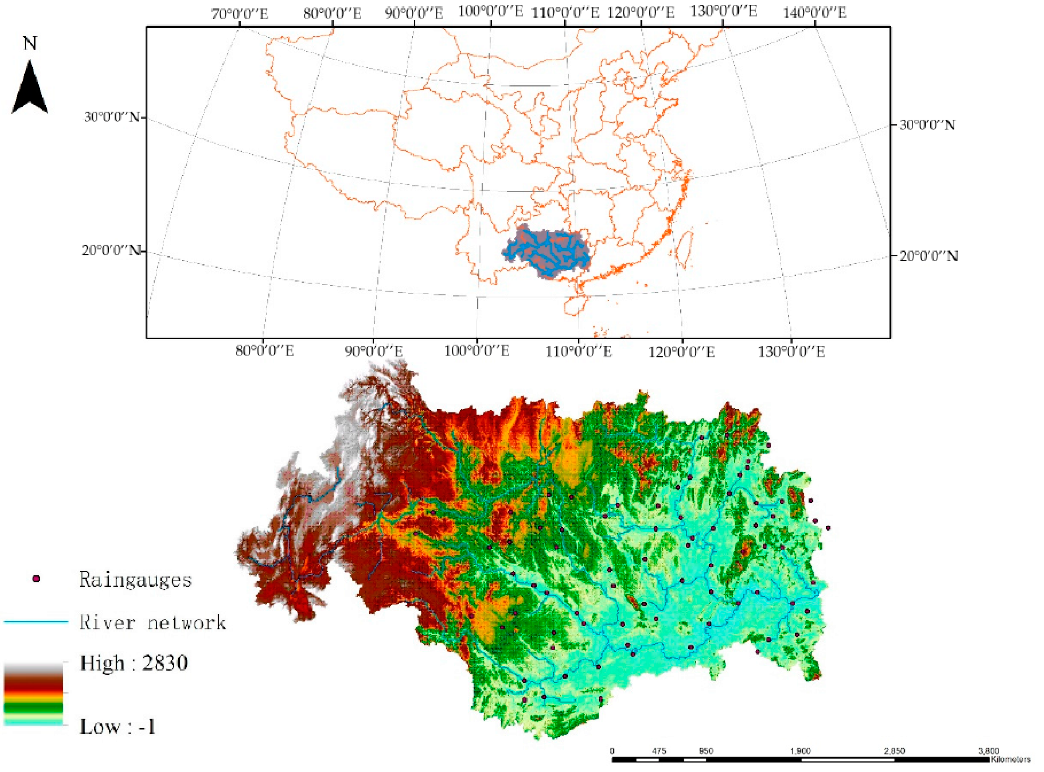
Figure 2.
Xinanjiang model structure (Zhao, 1992) [23].
Figure 2.
Xinanjiang model structure (Zhao, 1992) [23].
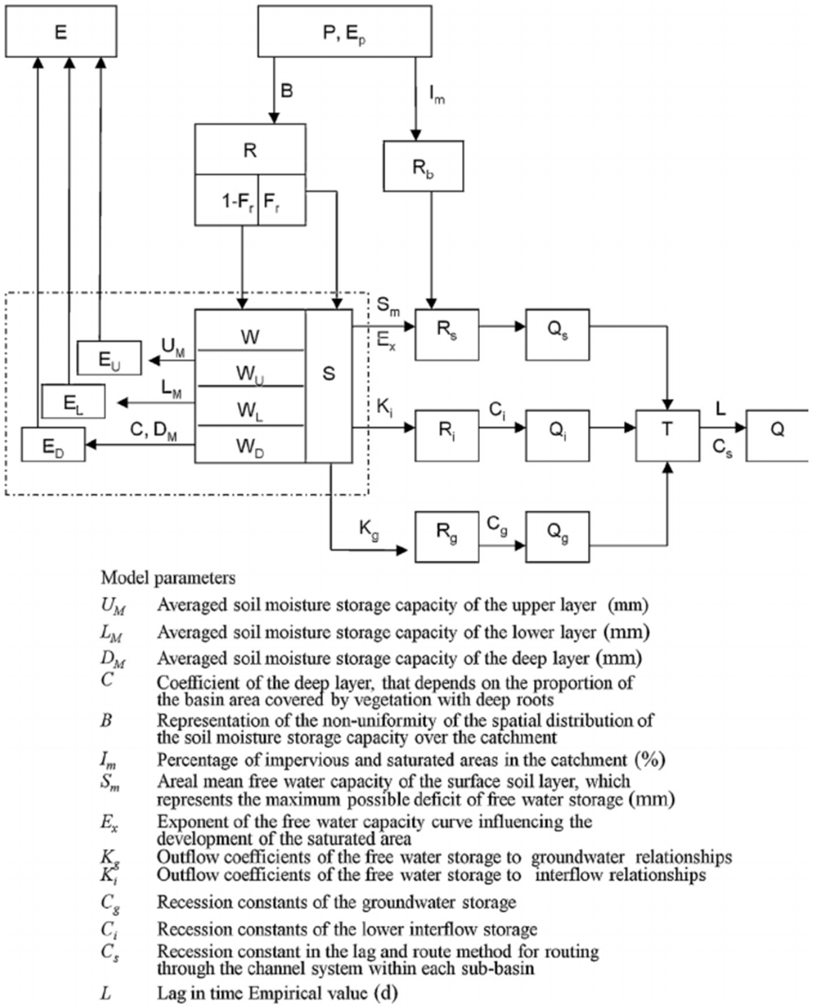
Figure 3.
Liuxihe model structure (Chen et al., 2010) [24].
Figure 3.
Liuxihe model structure (Chen et al., 2010) [24].
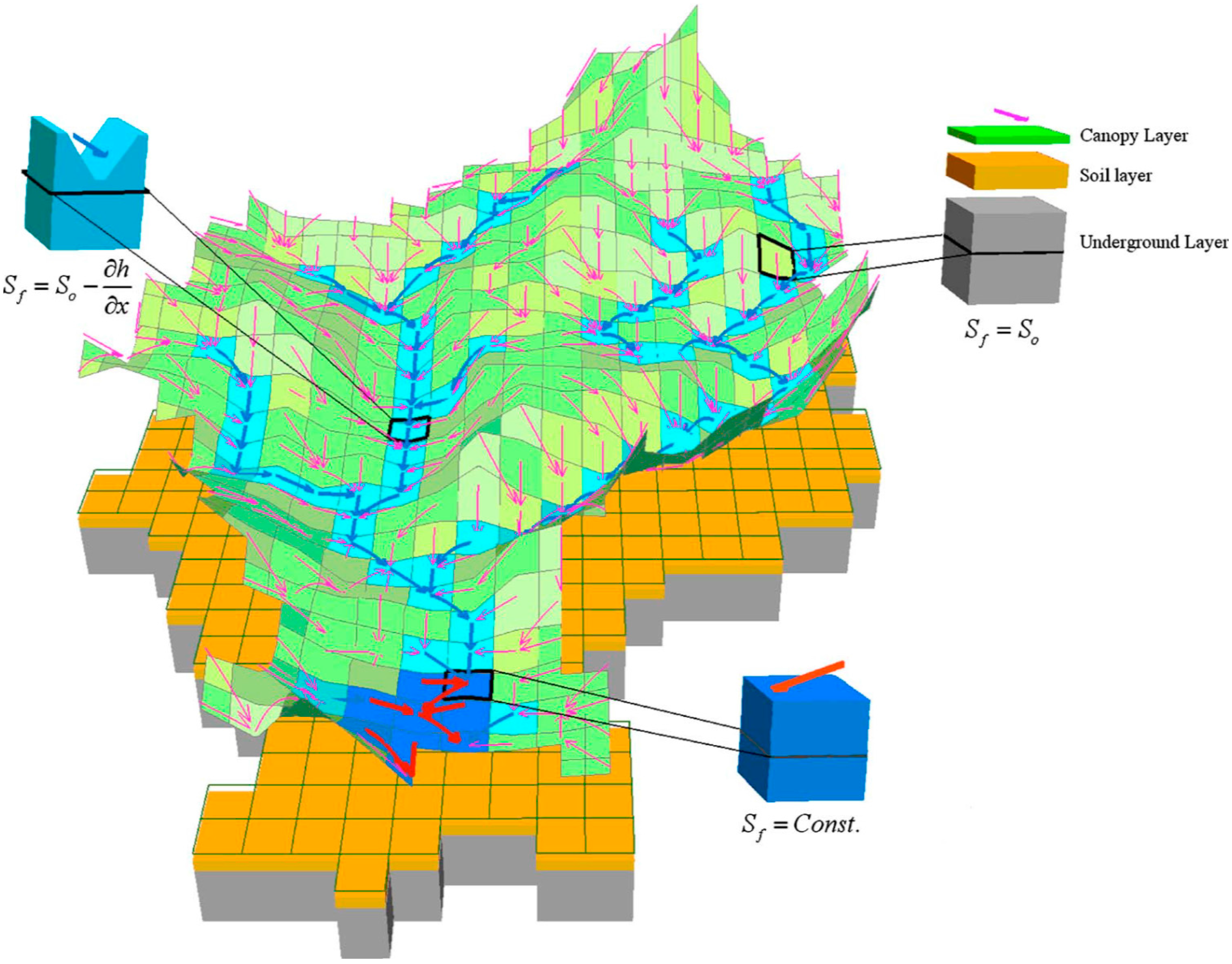
Figure 4.
The distribution of Regional Climate Model (RCM) grids on the Xijiang Basin.

Figure 5.
Comparison of cumulative catchment rainfall between historical rainfall from the climate model and rain gauge measurements.
Figure 5.
Comparison of cumulative catchment rainfall between historical rainfall from the climate model and rain gauge measurements.

Figure 6.
RF and rain gauge measurements in scatter map.
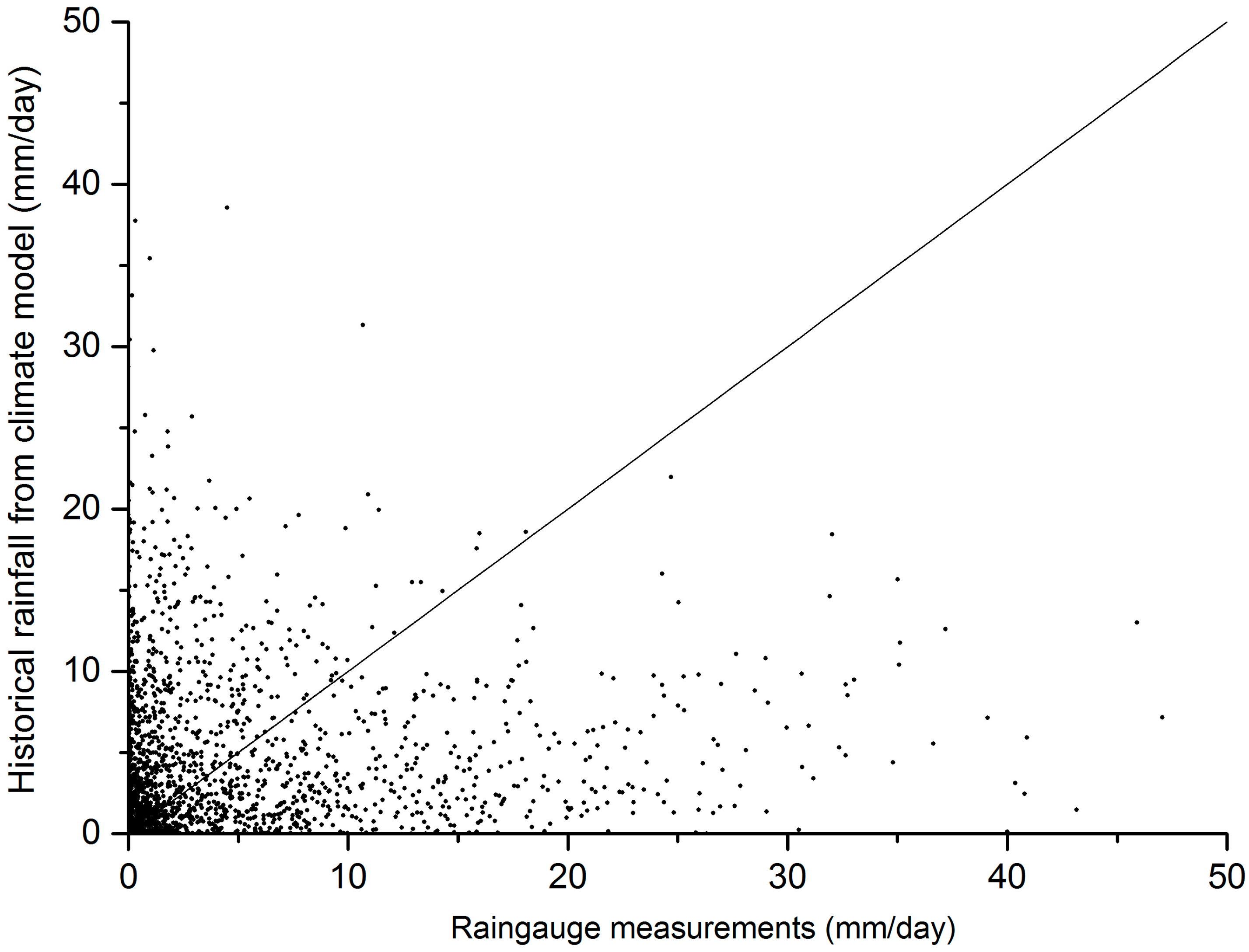
Figure 7.
Comparison of flow simulations in the XAJ model driven by historical rainfall from climate models and rain gauge measurements.
Figure 7.
Comparison of flow simulations in the XAJ model driven by historical rainfall from climate models and rain gauge measurements.

Figure 8.
Comparison of flow simulation in the LXH model driven by historical rainfall from climate models and rain gauge measurements.
Figure 8.
Comparison of flow simulation in the LXH model driven by historical rainfall from climate models and rain gauge measurements.
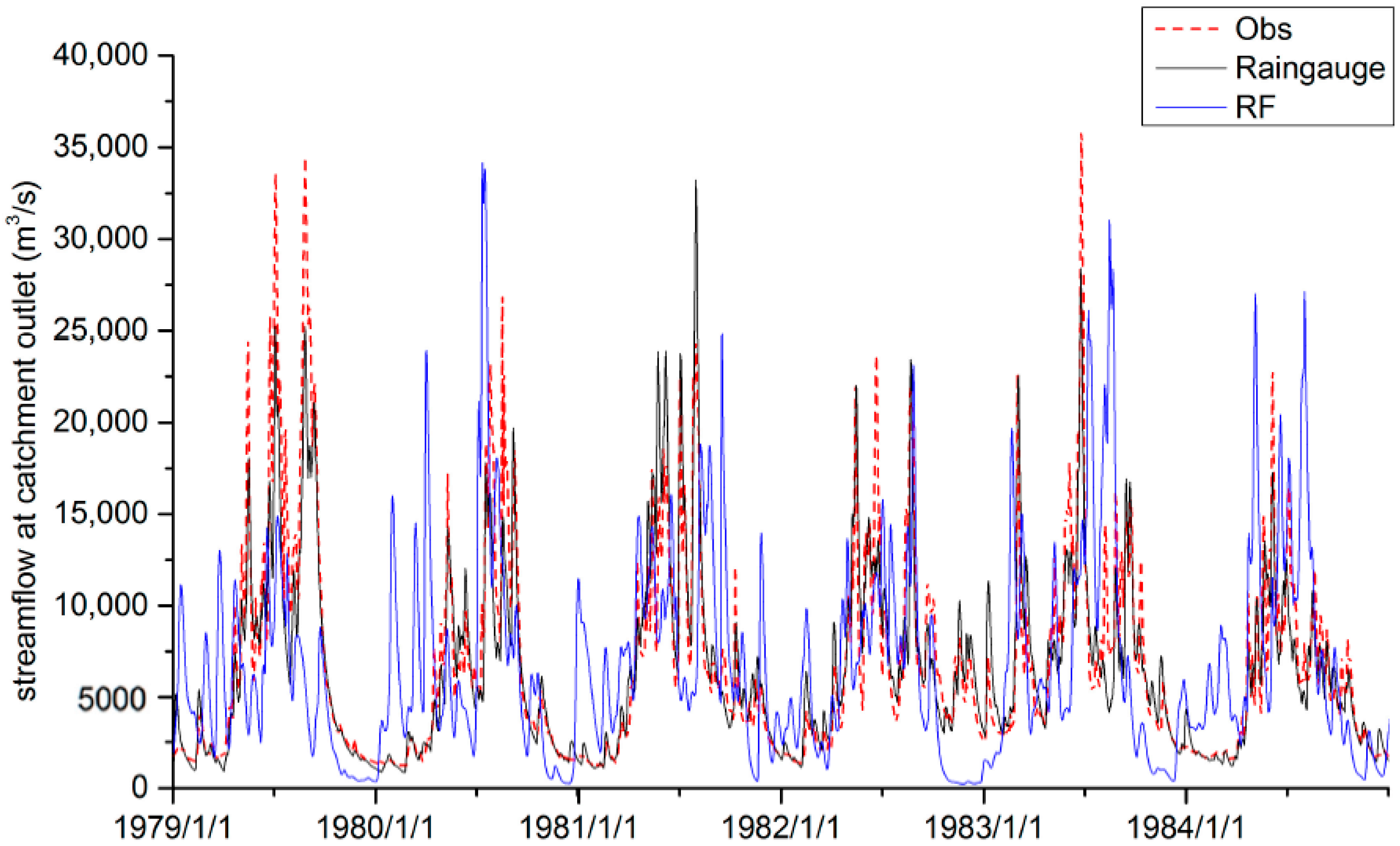
Figure 9.
Illustration of the box plot for monthly flow simulation results driven by representative concentration pathways (RCP) rainfall in the LXH model (a: RCP4.5; b: RCP8.5).
Figure 9.
Illustration of the box plot for monthly flow simulation results driven by representative concentration pathways (RCP) rainfall in the LXH model (a: RCP4.5; b: RCP8.5).

Figure 10.
Illustration of the box plot for monthly flow simulation results driven by representative concentration pathways (RCP) rainfall in the XAJ model (a: RCP4.5; b: RCP8.5).
Figure 10.
Illustration of the box plot for monthly flow simulation results driven by representative concentration pathways (RCP) rainfall in the XAJ model (a: RCP4.5; b: RCP8.5).
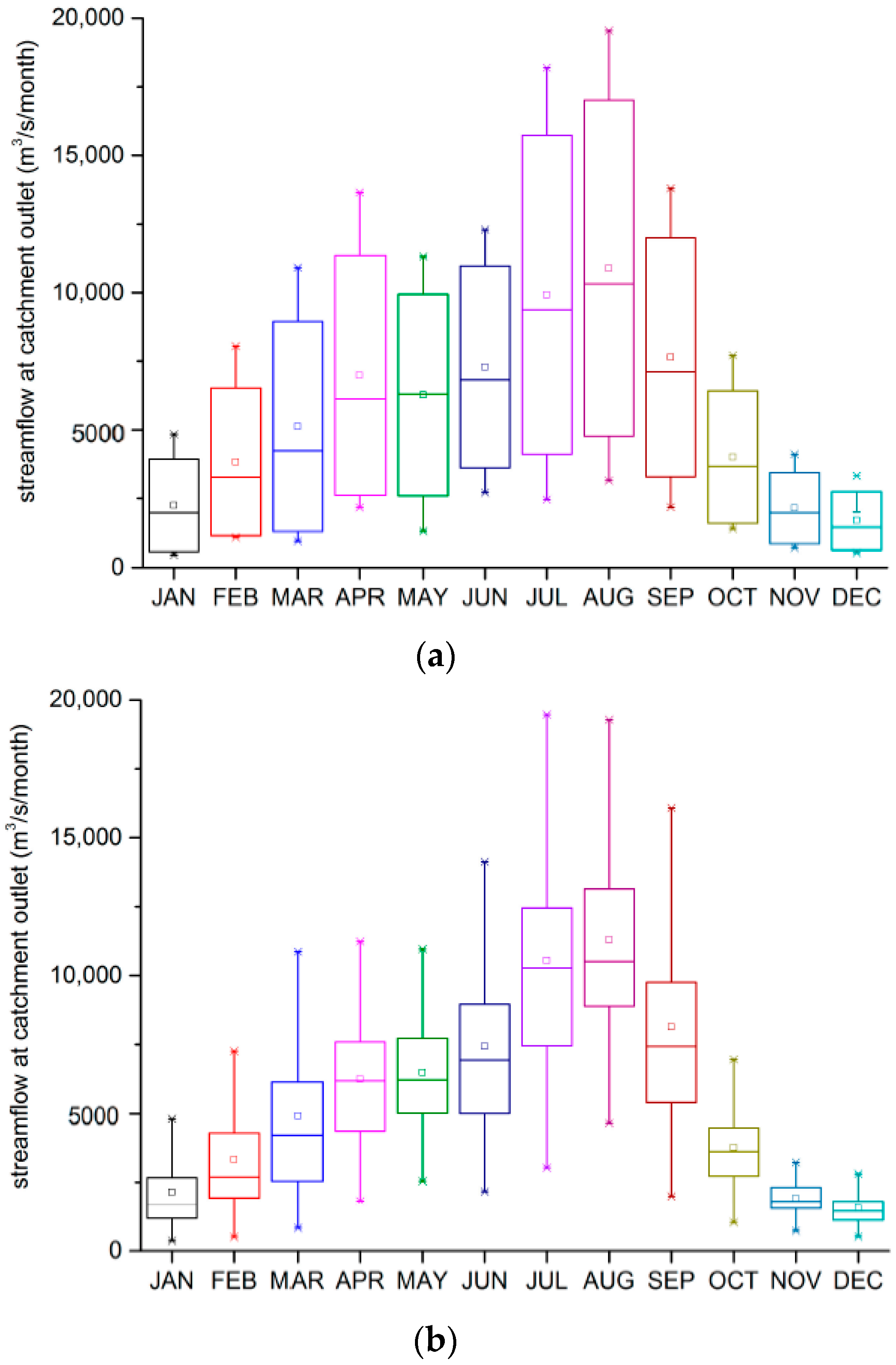
Figure 11.
Comparisons of median monthly rainfall and flow simulation under two climate change scenarios in two hydrological models (a: median monthly rainfall; b: median monthly streamflow).
Figure 11.
Comparisons of median monthly rainfall and flow simulation under two climate change scenarios in two hydrological models (a: median monthly rainfall; b: median monthly streamflow).
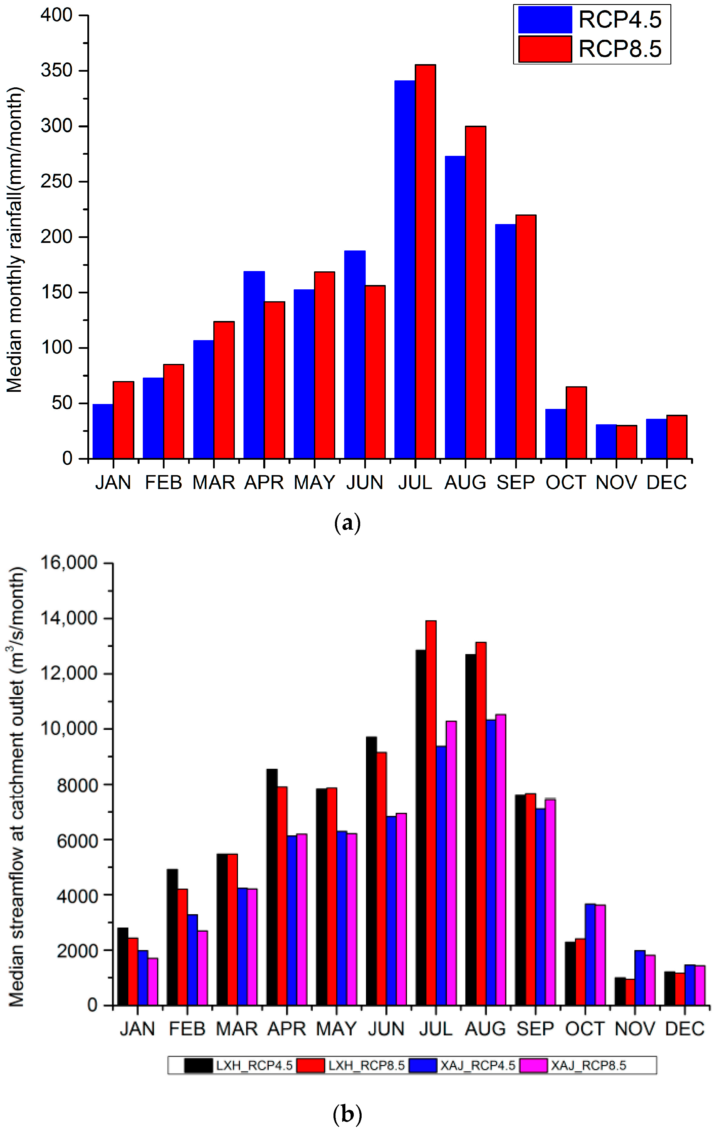
Figure 12.
Comparisons of annual flow simulation under two climate change scenarios in two hydrological models.
Figure 12.
Comparisons of annual flow simulation under two climate change scenarios in two hydrological models.
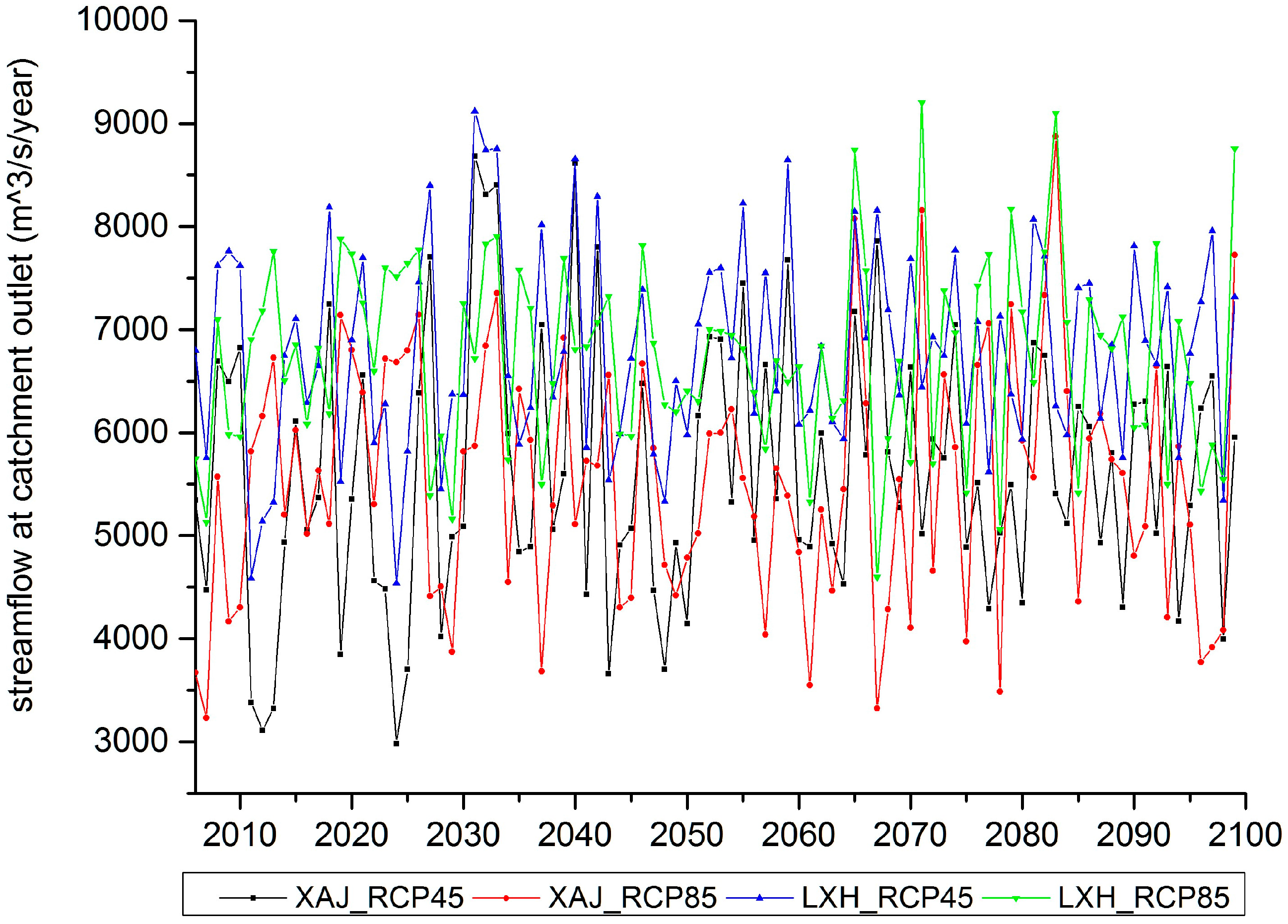
Figure 13.
Comparisons of flood magnitude under two climate change scenarios in two hydrological models based on the return period.
Figure 13.
Comparisons of flood magnitude under two climate change scenarios in two hydrological models based on the return period.


Table 1.
Statistics of the LXH and XAJ model calibration and validation.
| Criterions | NS | Cor | RMSE | PF | MSLE | |||||
|---|---|---|---|---|---|---|---|---|---|---|
| LXH | XAJ | LXH | XAJ | LXH | XAJ | LXH | XAJ | LXH | XAJ | |
| Calibration | 0.80 | 0.89 | 0.92 | 0.95 | 2898 | 2072 | –1.9% | –3.1% | 0.52 | 0.11 |
| Validation 1 | 0.81 | 0.83 | 0.92 | 0.91 | 2513 | 2365 | –5.3% | –8.6% | 0.56 | 0.08 |
| Validation 2 | 0.60 | 0.72 | 0.92 | 0.93 | 3298 | 2721 | 15% | 18.1% | 0.66 | 0.17 |
Table 2.
Statistics for projected monthly flow simulations using the LXH model (unit: m3/s).
| Jan. | Feb. | Mar. | Apr. | May | Jun. | Jul. | Aug. | Sep. | Oct. | Nov. | Dec. | |
|---|---|---|---|---|---|---|---|---|---|---|---|---|
| RCP4.5 | ||||||||||||
| Min | 429 | 1042 | 645 | 3410 | 3144 | 3955 | 4249 | 4764 | 2711 | 339 | 243 | 268 |
| Q1 | 1610 | 3750 | 3782 | 6536 | 6604 | 7232 | 10,512 | 10,712 | 5483 | 1415 | 583 | 609 |
| Median | 2792 | 4917 | 5470 | 8545 | 7826 | 9702 | 12,850 | 12,692 | 7599 | 2282 | 991 | 1199 |
| Q3 | 4065 | 6557 | 8807 | 10,619 | 9280 | 12,536 | 15,967 | 16,267 | 9896 | 4317 | 2032 | 1857 |
| Max | 6630 | 10,550 | 14,131 | 16,013 | 11,810 | 19,743 | 23,287 | 23,715 | 15,834 | 8285 | 3721 | 3662 |
| RCP8.5 | ||||||||||||
| Min | 208 | 518 | 1118 | 1934 | 3225 | 3741 | 4982 | 6077 | 1518 | 430 | 255 | 211 |
| Q1 | 1357 | 2831 | 3668 | 5910 | 6740 | 6544 | 10,607 | 10,680 | 4882 | 1487 | 603 | 688 |
| Median | 2437 | 4193 | 5475 | 7903 | 7870 | 9147 | 13,916 | 13,132 | 7658 | 2405 | 931 | 1156 |
| Q3 | 3705 | 6467 | 8215 | 9824 | 10,050 | 11,623 | 16,507 | 15,731 | 10,835 | 3593 | 1638 | 1681 |
| Max | 6714 | 11,071 | 12,783 | 14,577 | 13,793 | 19,055 | 25,257 | 21,240 | 17,868 | 6734 | 2884 | 3130 |
Table 3.
Statistic of projected monthly flow simulation using the XAJ model (unit: m3/s).
| Jan. | Feb. | Mar. | Apr. | May | Jun. | Jul. | Aug. | Sep. | Oct. | Nov. | Dec. | |
|---|---|---|---|---|---|---|---|---|---|---|---|---|
| RCP4.5 | ||||||||||||
| Min | 452 | 1085 | 956 | 2168 | 1312 | 2709 | 2458 | 3146 | 2179 | 1384 | 707 | 534 |
| Q1 | 1237 | 2172 | 2927 | 4550 | 4776 | 5342 | 7451 | 7990 | 5557 | 2561 | 1408 | 1126 |
| Median | 1977 | 3274 | 4230 | 6127 | 6297 | 6827 | 9375 | 10,323 | 7109 | 3663 | 1976 | 1451 |
| Q3 | 2748 | 4588 | 6596 | 8445 | 7630 | 9266 | 12,114 | 13,425 | 9556 | 4698 | 2536 | 2005 |
| Max | 4838 | 8050 | 10,908 | 13,647 | 11,315 | 12,305 | 18,193 | 19,545 | 13,801 | 7712 | 4103 | 3324 |
| RCP8.5 | ||||||||||||
| Min | 356 | 496 | 819 | 1817 | 2540 | 2161 | 3036 | 4650 | 1989 | 1024 | 723 | 517 |
| Q1 | 1175 | 1938 | 2546 | 4357 | 5014 | 5005 | 7455 | 8893 | 5398 | 2732 | 1525 | 1106 |
| Median | 1706 | 2690 | 4209 | 6190 | 6216 | 6940 | 10,281 | 10,514 | 7437 | 3620 | 1810 | 1422 |
| Q3 | 2672 | 4286 | 6138 | 7593 | 7722 | 8957 | 12,449 | 13,145 | 9762 | 4476 | 2312 | 1804 |
| Max | 4816 | 7264 | 10,868 | 11,241 | 10,965 | 14,122 | 19,467 | 19,285 | 16,082 | 6960 | 3231 | 2809 |
© 2017 by the authors. Licensee MDPI, Basel, Switzerland. This article is an open access article distributed under the terms and conditions of the Creative Commons Attribution (CC BY) license (http://creativecommons.org/licenses/by/4.0/).
Share and Cite
MDPI and ACS Style
Zhu, D.; Das, S.; Ren, Q. Hydrological Appraisal of Climate Change Impacts on the Water Resources of the Xijiang Basin, South China. Water 2017, 9, 793. https://doi.org/10.3390/w9100793
AMA Style
Zhu D, Das S, Ren Q. Hydrological Appraisal of Climate Change Impacts on the Water Resources of the Xijiang Basin, South China. Water. 2017; 9(10):793. https://doi.org/10.3390/w9100793
Chicago/Turabian StyleZhu, Dehua, Samiran Das, and Qiwei Ren. 2017. "Hydrological Appraisal of Climate Change Impacts on the Water Resources of the Xijiang Basin, South China" Water 9, no. 10: 793. https://doi.org/10.3390/w9100793
Note that from the first issue of 2016, this journal uses article numbers instead of page numbers. See further details here.