Optimization Strategy for Improving the Energy Efficiency of Irrigation Systems by Micro Hydropower: Practical Application

Abstract

Analyses of possible synergies between energy recovery and water management are essential for achieving sustainable advances in the performance of pressurized irrigation networks. Nowadays, the use of micro hydropower in water systems is being analysed to improve the overall energy efficiency. In this line, the present research is focused on the proposal and development of a novel optimization strategy for increasing the energy efficiency in pressurized irrigation networks by energy recovering. The recovered energy is maximized considering different objective functions, including feasibility index: the best energy converter must be selected, operating in its best efficiency conditions by variation of its rotational speed, providing the required flow in each moment. These flows (previously estimated through farmers’ habits) are compared with registered values of flow in the main line with very suitable calibration results, getting a Nash–Sutcliffe value above 0.6 for different time intervals, and a PBIAS index below 10% in all time interval range. The methodology was applied to a Vallada network obtaining a maximum recovered energy of 58.18 MWh/year (41.66% of the available energy), improving the recovered energy values between 141 and 184% when comparing to energy recovery considering a constant rotational speed. The proposal of this strategy shows the real possibility of installing micro hydropower machines to improve the water–energy nexus management in pressurized systems.

1. Introduction

Modern society is increasingly aware of the need to improve energy efficiency across all industrial sectors and processes. Increased sustainability can be achieved through the development of renewable energy sources such as photovoltaic, wind, tidal or hydropower. To reach this sustainable growth, deep management is necessary [1]. Water distribution systems, particularly irrigation systems, have not been included in this trend, considering that these infrastructures are high energy consumers regarding the captation, distribution and reuse of water resources. The importance of hydraulic systems as energy consumers is shown through the worldwide consumption of energy, in which the energy consumption for water supply networks represents 7% of the total consumed energy [2]. If this value is discretized, the distribution is approximately one-third (2–3%) of this consumption [3].

Therefore, considering the need to develop sustainable growth in water systems [4] since the distribution of water is an intensive energy process [5], new strategies should be introduced for water management systems. The aim of these strategies has to be the improvement of the energy efficiency and the decrease of the carbon footprint [6], considering the basic principles for the integration of the water and carbon footprints cost into the resource and environmental costs respectively [7,8,9], as well as newly available technologies that improve the water management of the resources and their feasibility [10,11]. These strategies must consider the flow variation over time in extended periods since the analysis of the long-extended period enables us to analyse the behaviour of the micro hydropower systems when the flow changes [12]. Hence, the installation of recovery systems is one of the most effective strategies to be used in places where the energy has to be dissipated (e.g., pressure reduction valves (PRVs) or hydraulic jumps [13,14,15]), with high feasibility indexes [16].

Deep knowledge of the water–energy nexus in hydraulic systems is essential to define and to introduce new action lines for their management in order to define performance indicators [17,18]. The analysis of the water–energy nexus, which depends on the intrinsic factors of the hydraulic systems, defines the potential energy recovery in any hydraulic system. Once the water–energy nexus is defined, the performance indicators can be established, quantifying the energy savings and contributing to the improvement of the sustainable, environmental, economic, and management components [19,20,21,22]. The improvement of these indicators was tackled for water systems using optimization analyses for the locations of the hydropower systems [23,24], as well as developing comparisons between different algorithms [25].

The present research is focused on contributing to the knowledge pertaining to the operating mode of energy recovery systems, when they are installed in pressurized water networks (particularly in irrigation networks). The aim of this research is centred on the proposal and development of a methodology to improve energy efficiency in pressurized irrigation networks. The improvement is achieved through the installation of micro hydropower turbines, which take advantage of the high pressure in some zones of the network by recovering the excess of the pressure-generating green energy. This is achieved by replacing pressure reduction valves, currently installed in the water systems to reduce the pressure by micro hydropower, reducing, as a consequence, leakages [26,27].

2. Methods and Materials in the Optimization Strategy

The development of a methodology to optimize the energy recovery in pressurized water systems is carried out, and the strategy is particularly applied to irrigation networks. Therefore, the research is defined by an ensemble of methodologies and materials, in which the results and their correlations constitute the methodology to optimize energy recovery in pressurized water systems.

2.1. Methods

The used methods were focused on (i) the definition of the analytical model to determine the flow over time; (ii) the strategy to validate the methodology to estimate the flow in each line of the network; (iii) the optimization of the recovered energy by an analytical strategy; (iv) the study of analytical models to know the efficiency in quasi-steady flow conditions when the demand changes using affinity laws for machine operating conditions; and (v) simulation of the analytical method by using a hydraulic numerical model to know the pressure and flow over time in each line.

The definition of the analytical model to determine the flow over time was focused on the determination of the opening or closing irrigation points, depending on the balance between the irrigation needs and the irrigation cumulated volume. The opening of an irrigation point was established on different patterns that show the irrigation trends of farmers, such as the weekly trend, the maximum days between irrigation, and the irrigation duration. The definition of these patterns enables us to determine the time for the start of irrigation.

The calibration strategy was based on key performance indicators (KPIFs), coming from traditional hydrological models [28,29]. The KPIFs were Nash–Sutcliffe (E), root relative square error (RRSE) and percent of bias (PBIAS). These calibration indicators enable us to determine the goodness-of-fit between estimated and registered flows.

The developed optimization was carried out in two phases by an analytical strategy. The first was focused on the integral balance of the energy in a control volume [30]. The energy terms were defined, distinguishing between recoverable and non-recoverable energy. The estimation of these terms depended on the required energy for irrigation. The second phase was proposed to develop an optimization strategy through a heuristic algorithm that was based on the analogy with the physics process of the annealing of metals and which inspired the Monte-Carlo method [31]. Based on this algorithm, preliminary studies were used to allocate three machines [32]. However, the recovered energy in a recovery system depended on the efficiency of the implemented hydraulic machine. The strategies of regulation that were defined by Carravetta et al. [33], were considered to determine the recovered energy since the flow varies over time in any water system. This management was based on the affinity laws and characteristic parameters of the hydraulic machines. The objective was to analyse the variation of head and efficiency curves as a function of the rotational speed when the machine operates under steady state conditions.

Once the analytical method had proposed the consumption patterns curves, simulations were developed to be applied to different case studies. The software used was EPANET [34] software, which is a public domain software that models water distribution in pipe systems. Different elements can be represented: pipe networks, nodes (junctions), pumps, valves, and storage tanks or reservoirs. The model can analyse extended-period, computing friction and minor losses; represent various types of valves, junctions, tanks and pumps; consider multiple patterns of node consumption over time; and operate the system of a simple tank level, timer controls or complex rule-based controls.

2.2. Materials

In this particular case, the materials are the experimental data, which were obtained along the development of this research. These materials were collected through different strategies: (i) the development of interviews to get to know the farmers’ habits. The data were used as input data in the analytical model that was developed to estimate the flow over time; (ii) the data for registered flow over the time of the irrigation network; (iii) the experimental curves based on the characteristic parameters (discharge and head number) as a function of the specific speed.

The interviews with farmers were developed in the irrigation community that is related to the case study. The results were afterwards used to determine the patterns to estimate the flow by the proposed methodology in the case study. The registered flow data were used to carry out the calibration strategy. The data were obtained by a flowmeter, which was installed in the main line of the analysed irrigation network.

The final materials used were the head-flow characteristic curve (Q-H) and the efficiency as a function of the flow (Q-η). However, other methodologies to model this performance have been implemented, since there were no available experimental values for the recovered head and the efficiency as a function of the flow for different rotational speeds to be used for modelling. Hence, the PAT will be characterized through the specific speed, the impeller diameter and the rotational speed. As a novelty, the next section describes the characterization of this hydraulic machine. The proposed method considers the best efficiency line (BEL) and the best efficiency head (BEH) as the strategy used to optimize the energy-recovering actions. BEL (Figure 1) is the line that establishes the maximum efficiency of one machine for a determined rotational speed and flow. BEH is the line that is associated with BEL and represents the recovered head when the efficiency is maximum for each rotational speed [35].

Characterization of the Hydraulic Machine

The characterization of the hydraulic machine is necessary in the optimization strategy. In this research, a synthetic PAT module is proposed based on characteristic parameters (head number ($\mathsf{\psi }$) and discharge number ($\mathsf{\phi }$) [36]) that are shown in Figure 2. These characteristic numbers are defined by Equations (1) and (2):

$$\mathsf{\phi }=\frac{Q}{N{D}^3}$$

(1)

$$\mathsf{\psi }=\frac{Hg}{N^2{D}^2}$$

(2)

where Q is the flow in m³/s; N is the rotational speed of the machine in rpm; and D is the impeller diameter in m.

The turbine characterization (Figure 3) is developed by the following the next steps:

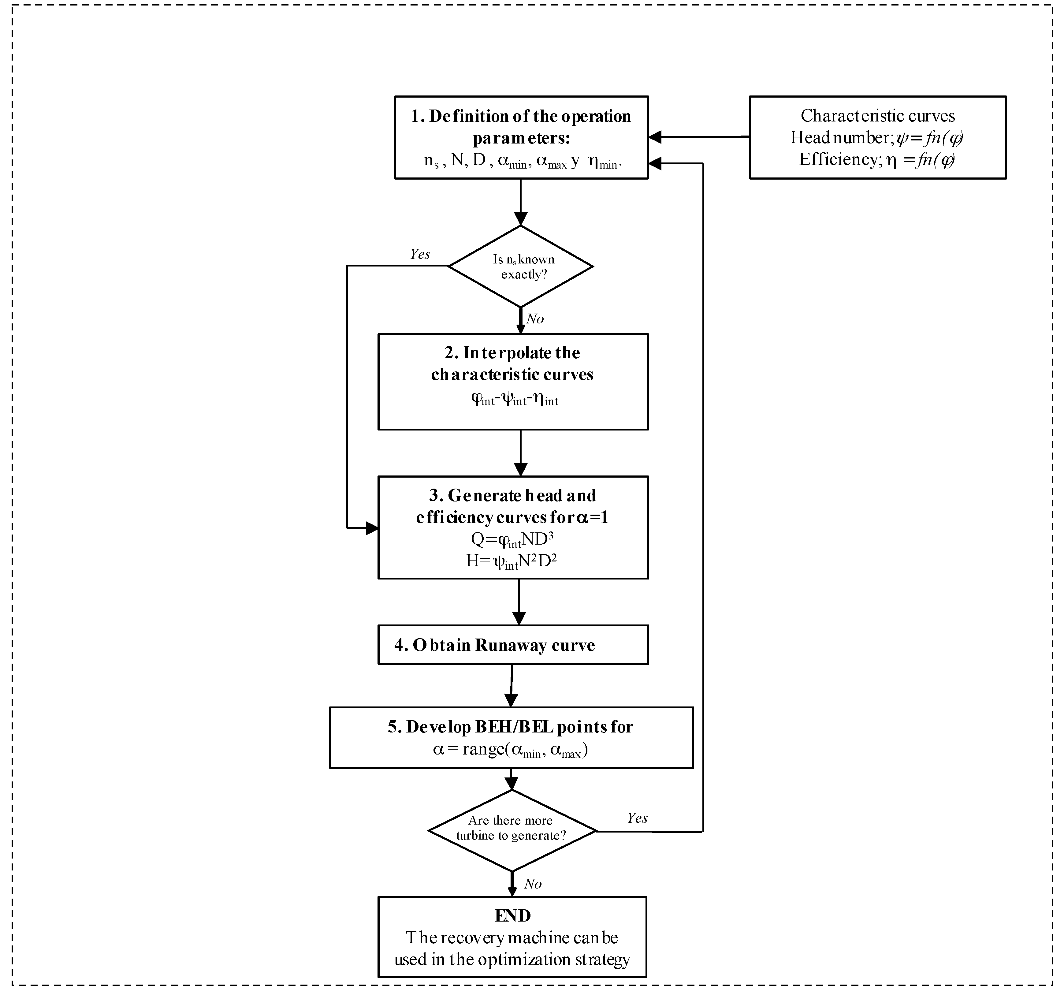
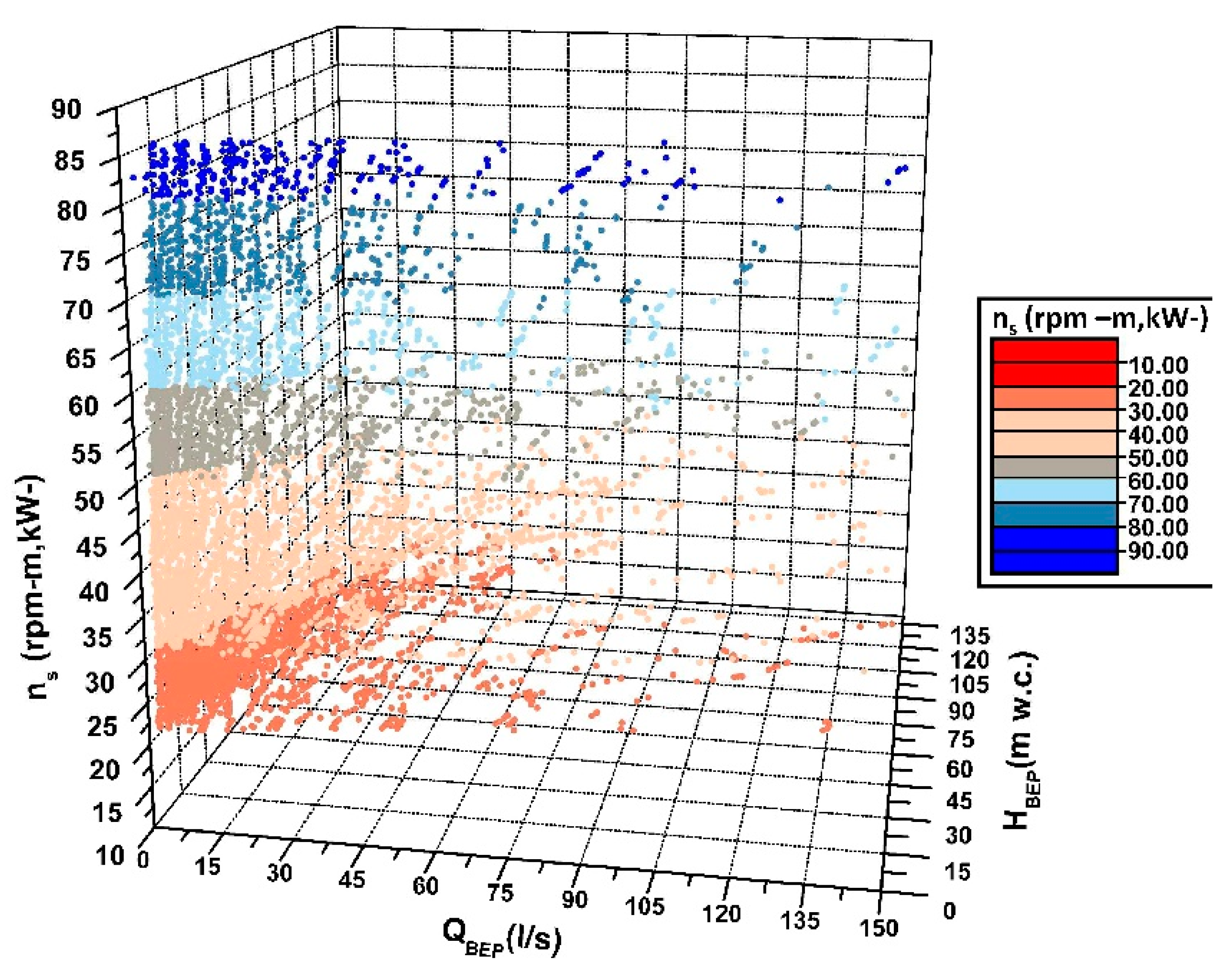
• Selection of the operation parameters: different parameters must be defined. To establish a database of synthetic PATs (in this particular case 8893 different PATs were defined). The database was developed through characteristic curves that are shown in Figure 2 (Input 1) as well as changing the following parameters:
  • Specific speed (n_s): defined according to Equation (3):

    $$n_s=N\frac{\sqrt{P_R}}{H_R^{1.25}}$$

    (3)

    where N is the rated rotational speed (rpm); P_R is the rated power (kW); H_R is the rated head (m w.c.); being ‘R’ the pump design point or the best efficiency condition.
    The range of specific speed oscillates between 14 and 79 rpm (m, kW).
  • Rotational speed (N): the range of the rotational speed oscillated between 510, 1020, 2040, 2400, and 2900 rpm.
  • Impeller Diameter (D): the range of the defined impeller was between 0.04 and 0.6 m.
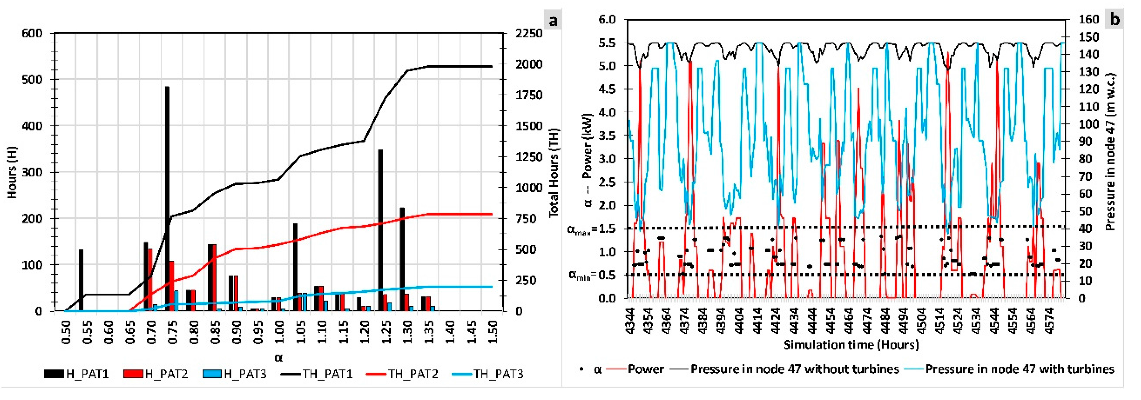
  • Variation of the rotational speed: when the machine operates with a different rotation speed as a function of the flow, the coefficient ($\mathsf{\alpha }$) that is defined by Equation (4) can vary between 0.5 and 1.5.

    $$\mathsf{\alpha }=\frac{N_t}{N_0}$$

    (4)

    where $N_t$ is the rotational speed for each time in rpm; and $N_0$ is the nominal rotational speed in rpm.
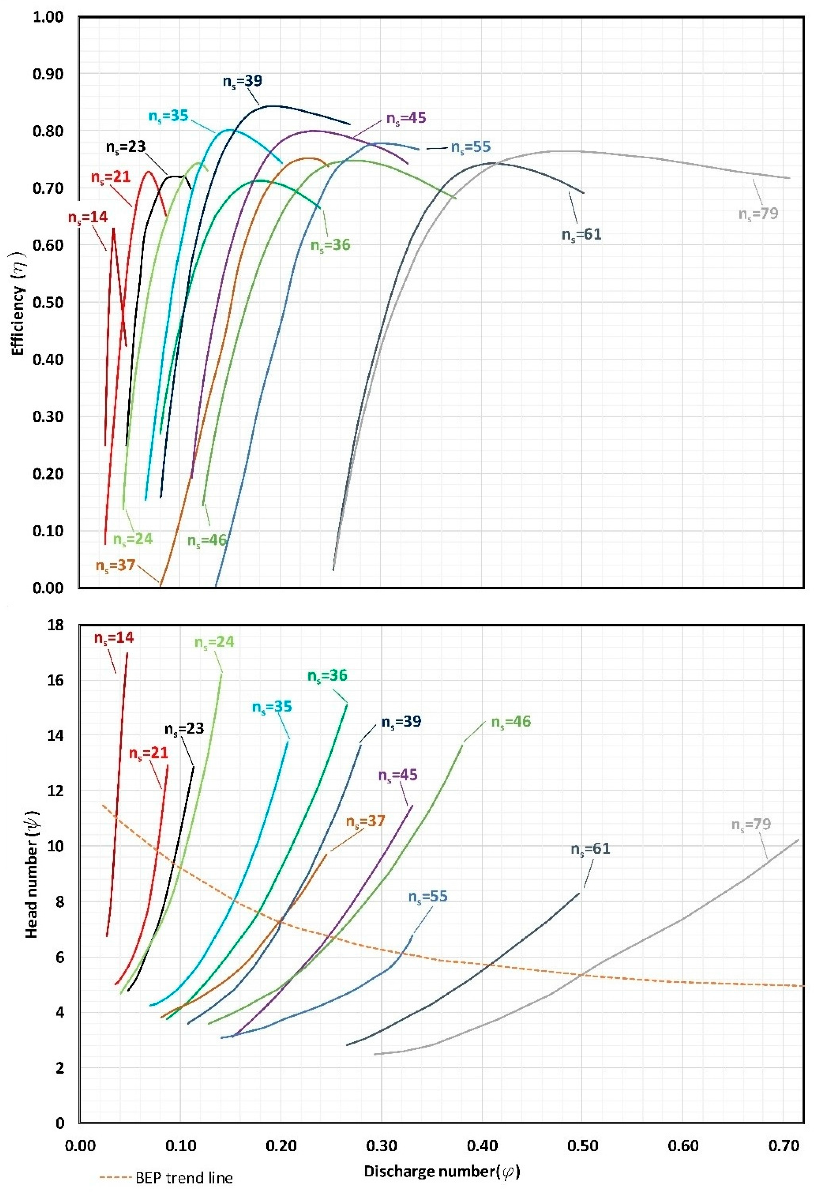
• To interpolate characteristic curves: when the specific speed is defined and the n_s curve is not known, the values of head number (${\mathsf{\psi }}_{int}$) and efficiency (η_int) for each discharge number value (φ_int) are estimated by linear interpolation
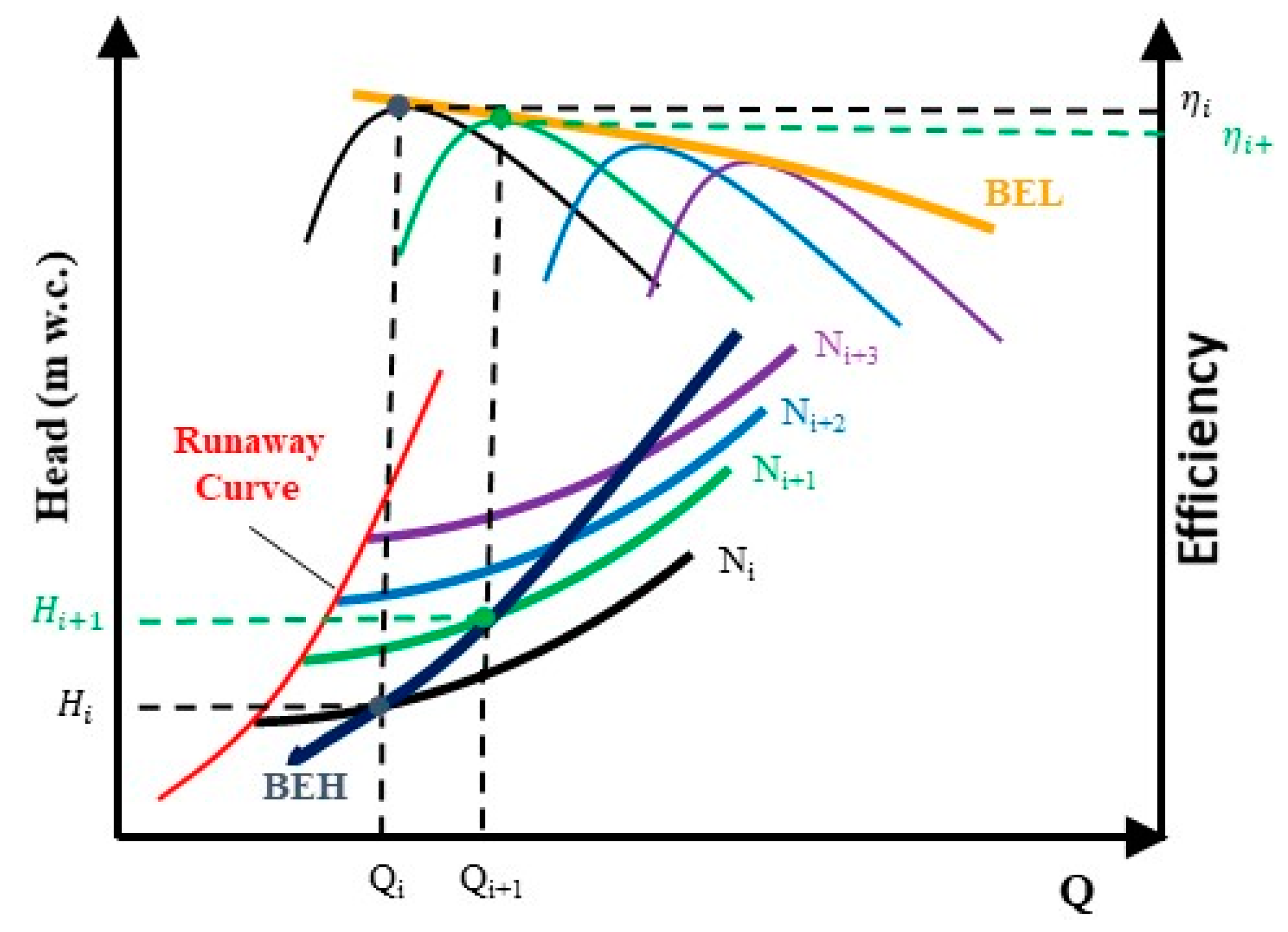
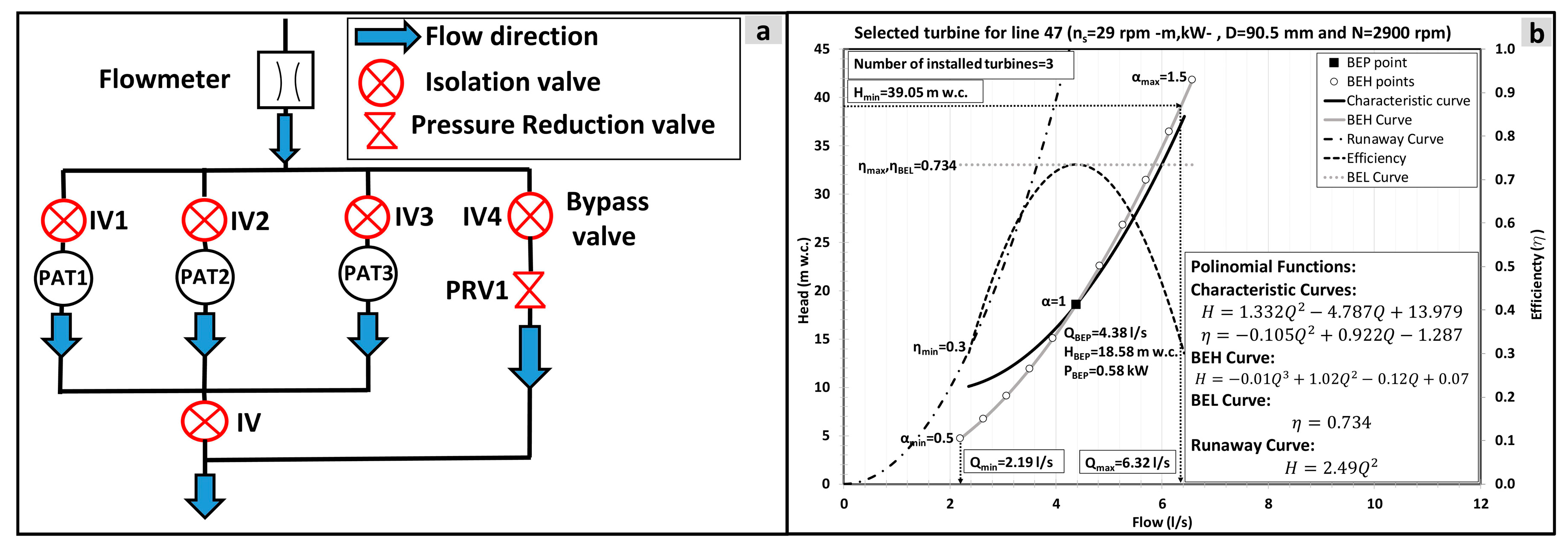
• To generate head and efficiency curves as a function of flow: when the characteristic numbers are defined for each diameter and rotational speed (N₀) that are selected in step one, the head and efficiency curve are determined by Equations (5) to (7):

  $$Q={\mathsf{\phi }}_{int}N{D}^3$$

  (5)

  $$H=\frac{{\mathsf{\psi }}_{int}{N}^2{D}^2}{g}$$

  (6)

  $$\mathsf{\eta }={\mathsf{\eta }}_{int}\left({\mathsf{\phi }}_{int}\right)$$

  (7)
  The polynomic equations are fitted to the obtained values (the maximum considered degree is four) through linear regression by Equations (8) and (9):

  $$H_{\mathsf{\alpha }=1}=A{Q}^4+B{Q}^3+C{Q}^2+DQ+E$$

  (8)

  $${\mathsf{\eta }}_{\mathsf{\alpha }=1}=F{Q}^4+G{Q}^3+H{Q}^2+IQ+J$$

  (9)
  These curves can be used when the flow is between the interpolated range, where A, B, C, D and E are coefficients of the Q-H characteristic curve and F, G, H, I and J are coefficients of the efficiency curve. The flow limit of the turbine is defined by a minimum efficiency condition, which is proposed to be 0.3 for this case study.
• To obtain runaway curve: the runaway curve is generated by second polynomic equation curve that contains the following points: coordinates origin and the minimum value obtained through Equation (8).
• To develop BEL/BEH: the best efficiency point is estimated for each rotational speed (α), adjusting by regression the curves defined by Equations (10) and (11):

  $$H_{BEH}=H{Q}^4+I{Q}^3+J{Q}^2+KQ+L$$

  (10)

  $${\mathsf{\eta }}_{BEL}=M{Q}^4+N{Q}^3+O{Q}^2+PQ+R$$

  (11)

  where H, I, J, K and L characterise the best efficiency head and M, N, O, P and R are coefficients that define the best efficiency line.

2.3. Optimization Strategy

When the previously-cited material and methods are implemented, the development of the optimization strategy to improve the energy efficiency in pressurized irrigation networks is possible. The development of this strategy makes sense since there are not any similar strategies for pressurized water distribution networks published in the expert literature. The developed optimization strategy for the energy efficiency improvement is defined by different steps. This methodology needs different inputs. The procedure is showed in the following flowchart (Figure 4).

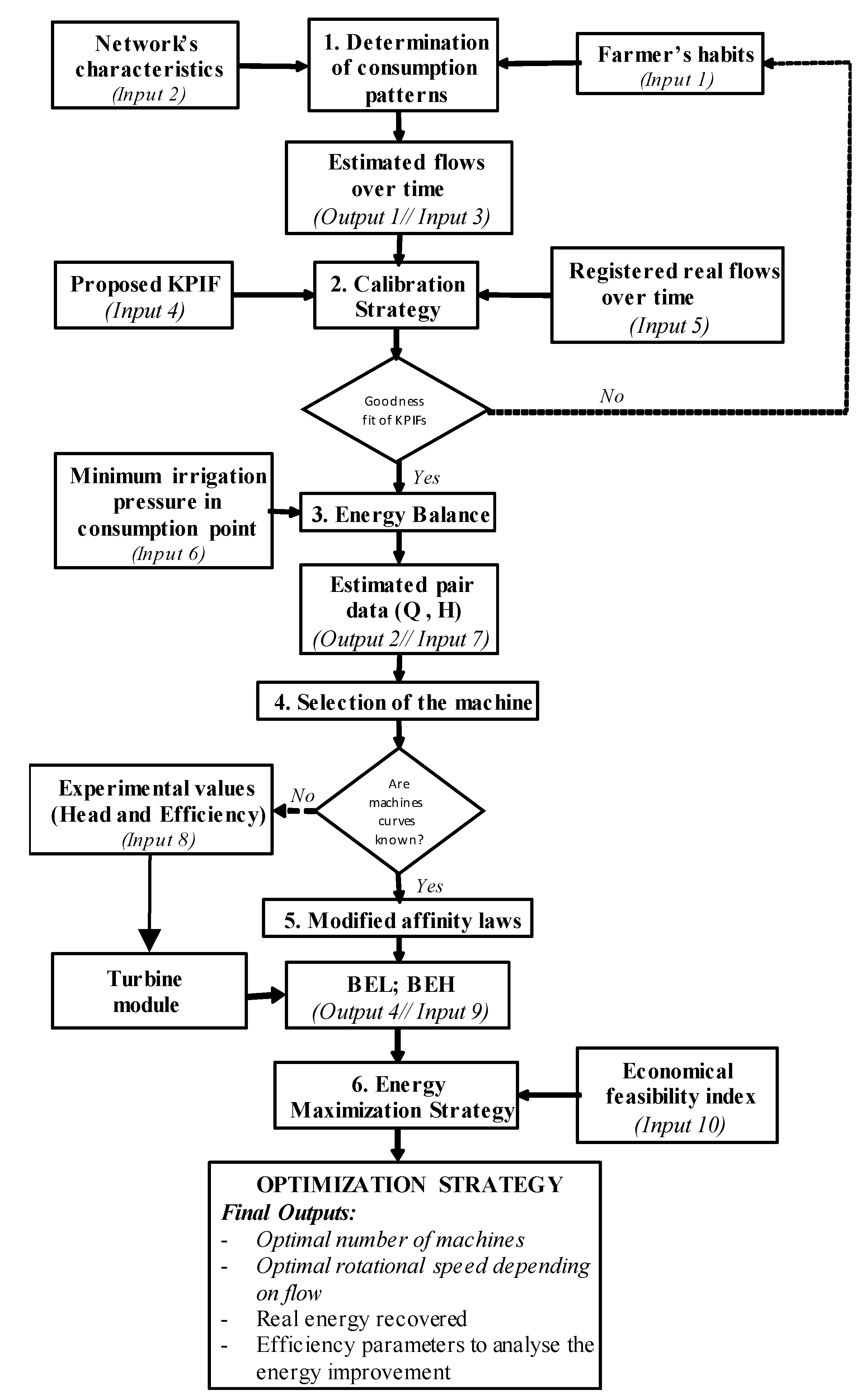
• The knowledge of the flow over time is the starting point in the optimization strategy. The flow can be known when the water manager has flowmeters in the pipes. However, the knowledge of the flow in all lines over time is almost impossible, and therefore, the flow has to be estimated in each line. In this sort of irrigation water distribution network, the flow depends on consumption flow patterns which must be determined as a function of the agronomist parameters. To estimate the consumption flow patterns, the used methodology considers the farmers’ habits and the characteristics of the network [39]. This methodology is able to estimate the flow over time in any line of the systems, depending on the network characteristics (Input 1) and the farmers’ habits (Input 2). The farmers’ habits are irrigation needs, irrigation duration, maximum days between irrigation and the irrigation volume. The knowledge of the farmers’ habits allows the determination of the opening or closing in consumption nodes over time. The state of the irrigation point determines the flow (Output 1) of the strategy. This output is an input for the next step: Input 3.
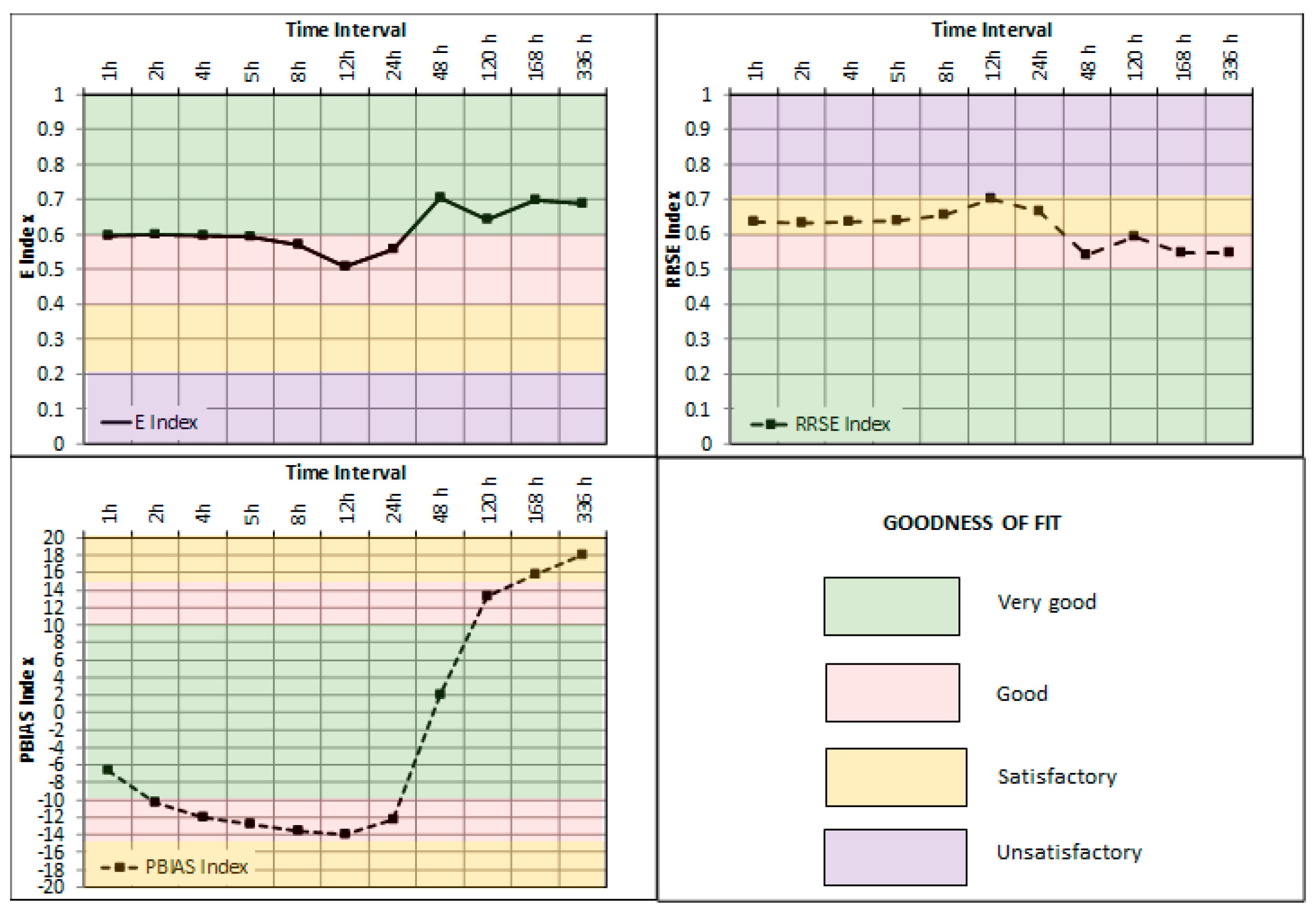
• The second stage stands on the calibration strategy. It uses key performance indicators (KPIFs) that are adapted from the traditional hydrological models (Input 4) [40]. The characterization of the goodness-of-fit is divided into very good, good, satisfactory, and unsatisfactory, depending on the KPIF values (

  Table 1. Classification of the goodness-of-fit (adapted from [40]).

  Goodness-of-Fit	E	RRSE	PBIAS (%)
  Very Good	E > 0.6	0.00 ≤ RRSE ≤ 0.50	$PBIAS<\pm 10$
  Good	0.40 < E ≤ 0.60	0.50 < RRSE ≤ 0.60	$\pm 10\le PBIAS<\pm 15$
  Satisfactory	0.20 < E ≤ 0.40	0.60 < RRSE ≤ 0.70	$\pm 15\le PBIAS<\pm 25$
  Unsatisfactory	E < 0.20	RRSE > 0.70	$PBIAS>\pm 25$

  ). The comparison is developed with the registered flow data (Input 5) to determine the success of the fit. If the calibration is satisfactory, the energy balance (Step 3) can be done.
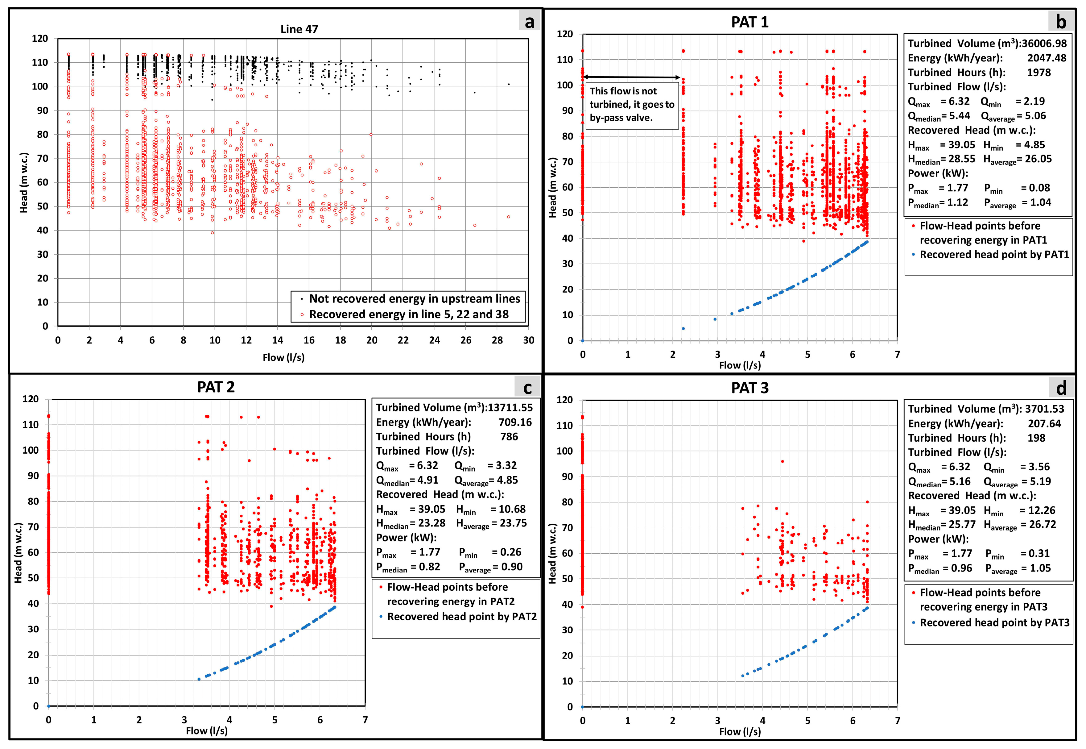
• The energy balance is able to discretize different energy terms (e.g., total, irrigation, friction) differentiating the terms for the available energy between the theoretically recoverable energy and theoretically non-recoverable energy, considering the minimum irrigation pressure at each consumption point (Input 6) [39]. The available energy enables us to determine the theoretical recovery coefficient at any line, hydrant or consumption point. In addition, the energy balance enables us to estimate the recovered head for each flow over time. Knowing these pairs of data (Q, H), the most suitable machine at each study point can be selected. The formula used to determine the annual balance of the network is defined by Equations (12) to (18):

  $$E_T=E_{FR}+E_{RI}+E_{TR}+E_{NTR}$$

  (12)

  $$E_{T_i}\left(\mathrm{kWh}\right)=\frac{9.81}{3600}{Q}_i\left(z_o-z_i\right)\Delta t$$

  (13)

  $$E_{F{R}_i}\left(\mathrm{kWh}\right)=2.725·{10}^{-3}{Q}_i\left(z_o-\left(z_i+P_i\right)\right)\Delta t$$

  (14)

  $$E_{R{I}_i}\left(\mathrm{kWh}\right)=2.725·{10}^{-3}{Q}_i{P}_{min{I}_i}\Delta t$$

  (15)

  $$E_{T{R}_i}\left(\mathrm{kWh}\right)=2.725·{10}^{-3}{Q}_i{H}_i\Delta t$$

  (16)

  $$E_{T{A}_i}\left(\mathrm{kWh}\right)=2.725·{10}^{-3}{Q}_i\left(P_i-P_{mi{n}_i}\right)\Delta t$$

  (17)

  $$E_{NT{R}_i}=E_{T{A}_i}-E_{T{R}_i}$$

  (18)

  where $E_T$ is the total provided energy in the network (kWh/year); $E_{FR}$ is the total friction energy in the network (kWh/year); $E_{RI}$ is the total required energy to irrigate correctly all consumption points (kWh/year); $E_{TR}$ is the total theoretical recovered energy in the network (kWh/year); $E_{NTR}$ is the total unrecoverable energy in the network (kWh/year); $E_{T_i}$ is the potential energy in each irrigation point when the consumption in the network is null (kWh); $E_{F{R}_i}$ is the dissipated friction energy until the irrigation point (kWh); $E_{R{I}_i}$ is the required energy at the consumption point to ensure the irrigation (kWh); $E_{T{A}_i}$ is the available energy for recovery in a hydrant or line (kWh); $E_{T{R}_i}$ is the maximum theoretical recoverable energy in an irrigation point, hydrant or line of the network, ensuring the minimum pressure of irrigation downstream (kWh); $E_{NT{R}_i}$ is the energy that cannot be recovered in a hydrant or line on the network (kWh); $Q_i$ is the flow by a line (m³/s); $z_i$ is the geometry level above reference plane of the irrigation point, considering the reference datum level (m); $z_{\mathrm{o}}$ is the geometry level above the reference plane of the free water surface of the reservoir (m); $P_i$ is the service pressure in any point of the network when consumption exists (m w.c.); $P_{min{I}_i}$ is the minimum pressure of service of an irrigation point required to ensure the irrigation water evenly; and $H_i$ is the value of the head of an irrigation point, hydrant or line (m w.c.). This head is obtained as $H_i=P_i-\max \left(P_{mi{n}_i};P_{min{I}_i}\right)$; and $\Delta t$ is the time interval (s).
• Knowing the flow ($Q_i$) and recoverable head ($H_i$) over time from the energy balance (Output 2, that is Input 7), enables the selection of the hydraulic machine type (e.g., radial, axial) according to the frequency histogram of the power generated among other conditions. To develop a guaranteed estimation of the recovered energy, the head and efficiency curve as a function of flow should be known for different rotational speeds (Input 8). If this information is not provided by the manufacturer, experimental tests are recommended to obtain the efficiency variation depending on the flow and for different rotational speeds. However, if experimental tests cannot be carried out, the experimental curves are determined using the characteristic numbers (discharge and head number, Figure 1) to select a machine considering its specific speed [41] using the turbine that was described in the previous section (Figure 2).
• When the tests are carried or the characteristic curves are used, the modified classical affinity laws based on the variation of the specific parameters (discharge coefficient, q; head coefficient, h; and velocity coefficient, n) can be used [33,42]. These parameters are defined by Equations (19) to (21):

  $$h=\frac{H}{H_0}$$

  (19)

  $$q=\frac{Q}{Q_0}$$

  (20)

  $$n=\frac{N}{N_0}$$

  (21)

  where H is the recovered head in m w.c.; Q is the flow through the turbine in m³/s when the rotational speed of the machine is N; and H₀ and Q₀ are head and flow, respectively, when the machine operates in its best efficiency point (BEP), for the rotational speed N₀.
  Based on modified classical similarity laws (when there are not experimental data), two new concepts (the best efficiency line, BEL and best head line, BEH) are proposed (Output 4). The BEL adapts the rotational speed as a function of the flow, adjusting the maximum efficiency at each time point and maximising the energy recovered. The BEH relates the best efficiency point for each rotational speed with the recovered head as a function of the flow [35]. The knowledge of the BEL and/or BEH (Input 9) makes possible the use of these curves to develop the optimization of the energy recovery on a water system through the variation of the rotational speed as a function of the flow. The classical laws are defined by Equations (22) to (24) [36]:

  $$\frac{Q_1}{Q_0}={\left(\frac{D_1}{D_0}\right)}^3\frac{N_1}{N_0}$$

  (22)

  $$\frac{H_1}{H_0}={\left(\frac{D_1}{D_0}\right)}^2{\left(\frac{N_1}{N_0}\right)}^2$$

  (23)

  $$\frac{P_1}{P_0}={\left(\frac{D_1}{D_0}\right)}^2{\left(\frac{N_1}{N_0}\right)}^3$$

  (24)

  where Q₁ is the flow in the new conditions of the rotational speed in m³/s; D₁ is the diameter of the impeller in the new N status in m; D₀ is the nominal diameter of the impeller in m; N₁ is the new rotational speed in rpm; H₁ is the head in the new N status in m w.c.; P₁ is the shaft power for each N in kW; and P₀ is the shaft power in the nominal condition in kW.
• This new strategy to maximize the energy recovered was developed by using PATs or any type of turbine. The theoretically recovered energy and the economic feasibility indexes (Input 10), particularly the simple payback period are considered (PSR) [39]. This strategy makes use of a simulated annealing algorithm to carry out the optimization, selecting the best lines to install turbines as a function of the number of installed turbines in the water system. The optimization can be developed with two different functions: the first function only considers the recovered energy, while the second one analyses the ratio between recovered energy and PSR [35]. The final output results of the optimization strategy are the optimal number of machines to install in the network according to the objective function; the optimal rotational speed as a function of the flow; the real recovered energy; as well as the efficiency parameters to analyse the energy improvement in the network.

3. Results and Discussion

The previously-described methodology was implemented in a real case study for an existing irrigation network. This network was located in Vallada (Valencia, Spain) and the water manager knew the volume measurements for the final user points as well as main line flow measurements over time.

3.1. Case Study Description

The Vallada network is a branched agronomic pressurized water distribution network, in which 30 m w.c. should be guaranteed at each irrigation point, so that farmers received quality water service (Figure 5). The dripped network had seventy hydrants, which supply 371 irrigation points. These irrigation points were connected by pipelines with diameters between 150 and 500 mm.

3.2. Results of the Optimization

Considering the farmers’ habits (Input 1) described by Pérez-Sánchez et al. (2016) [39] for the Vallada network, the flow was estimated over time, applying the proposed methodology and considering a time interval of 5 min [39]. After this, the maximum flow in the selected time interval was compared with the registered maximum flow for each time interval in the year 2015. The calibration was done for the maximum flow to determine whether the methodology produced a good or bad estimation, since the flow range is necessary in order to select the machines. When the calibration strategy was applied to this case study, the results were satisfactory according to the KPIFs in Table 1. The goodness-of-fit is set out in Figure 6.

According to Table 1, the results performance was very good (0.6) when the time interval was between 1 and 5 h. When the time interval varied from 8 to 24 h, E values were between 0.50 and 0.56. The performance was always very good when the time interval was greater than 24 h. RRSE values were also analysed, and the goodness-of-fit was satisfactory when the time interval was between 1 and 24 h. If the time interval was above 24 h, the performance was good. Finally, when the PBIAS index was analysed, the goodness-of-fit was very good for 1, 2, and 48 h. The calibration stage obtained a good fit when the time interval was between 4 and 24 h. Satisfactory results were obtained when the time interval was 168 and 336 h.

Once the goodness-of-fit was verified using the KPIFs, the energy balance was applied. To do so, the proposed optimization strategy combined the energy balance (Step 3 in Figure 5); the selection of the machine (Step 4 in Figure 5), which is chosen through the database created using the proposed turbine generated (Figure 7); the modified affinity laws (Point 5 in Figure 5); and the maximization strategy (Step 6 in Figure 5) developed by simulated annealing algorithm.

When the optimization strategy was performed, the recovered energy was maximized by selecting the machines operating under the best efficiency line.

Table 2. Results of the maximization of the recovered energy (n is the number of pipes where the turbines are installed; n_s in rpm (m, kW); D in mm; N in rpm; $E_{R_{BEL}}$ in MWh/year).

n		Lines in Which Turbines Are Allocated
1		38
2		22	38
3		22	38	59
4		22	38	47	59
5		5	22	38	47	59
6		5	22	38	47	58	59
7		5	22	38	47	58	59	70
8		5	22	38	39	47	58	59	70
9		2	10	22	39	43	47	58	59	70
10		2	10	22	39	43	47	58	59	70	85
n												Total ${\mathit{E}}_{{\mathit{R}}_{\mathit{B}\mathit{E}\mathit{L}}}$
1	ns D N ${\mathit{E}}_{{\mathit{R}}_{\mathit{B}\mathit{E}\mathit{L}}}$	35 114.3 2900 33.78										33.78
2	ns D N ${\mathit{E}}_{{\mathit{R}}_{\mathit{B}\mathit{E}\mathit{L}}}$	35 133.8 2900 30.97	35 134.9 2900 11.59									42.55
3	ns D N ${\mathit{E}}_{{\mathit{R}}_{\mathit{B}\mathit{E}\mathit{L}}}$	35 133.8 2900 30.97	35 134.9 2900 11.59	35 122.9 2900 3.56								46.11
4	ns D N ${\mathit{E}}_{{\mathit{R}}_{\mathit{B}\mathit{E}\mathit{L}}}$	35 133.8 2900 30.97	35 134.9 2900 11.59	29 90.5 2900 2.96	35 122.9 2900 3.56							49.08
5	ns D N ${\mathit{E}}_{{\mathit{R}}_{\mathit{B}\mathit{E}\mathit{L}}}$	44 175.7 2040 9.81	35 164.7 2900 24.16	35 134.9 2900 11.52	29 90.5 2900 2.96	35 122.9 2900 3.56						52.00
6	ns D N ${\mathit{E}}_{{\mathit{R}}_{\mathit{B}\mathit{E}\mathit{L}}}$	44 175.7 2040 9.81	35 164.7 2900 24.16	35 134.9 2900 11.52	29 90.5 2900 2.96	35 100.6 2900 2.64	40 121.2 2900 3.52					54.60
7	ns D N ${\mathit{E}}_{{\mathit{R}}_{\mathit{B}\mathit{E}\mathit{L}}}$	44 175.7 2040 9.81	35 164.7 2900 24.16	35 134.9 2900 11.52	29 90.5 2900 2.96	35 100.6 2900 2.64	35 122.9 2900 3.56	24 77 2900 0.83				55.47
8	ns D N ${\mathit{E}}_{{\mathit{R}}_{\mathit{B}\mathit{E}\mathit{L}}}$	44 175.7 2040 9.81	35 164.7 2900 24.16	35 134.9 2900 11.52	24 60.4 2900 1.05	29 90.5 2900 2.96	35 100.6 2900 2.64	35 122.9 2900 3.56	24 77 2900 0.83			56.53
9	ns D N ${\mathit{E}}_{{\mathit{R}}_{\mathit{B}\mathit{E}\mathit{L}}}$	83 118.3 2900 8.27	35 243.7 1020 6.22	35 164.7 2900 20.38	24 77 2900 1.46	35 134.9 2900 10.73	29 90.5 2900 2.96	35 100.6 2900 2.64	35 122.9 2900 3.56	24 77 2900 0.83		57.04
10	ns D N ${\mathit{E}}_{{\mathit{R}}_{\mathit{B}\mathit{E}\mathit{L}}}$	83 118.3 2900 8.27	35 243.7 1020 6.22	35 164.7 2900 20.38	24 77 2900 1.46	35 134.9 2900 10.73	29 90.5 2900 2.96	35 100.6 2900 2.64	35 122.9 2900 3.56	24 77 2900 0.83	26 71.5 2900 1.14	58.18

shows from 1 to 10 lines of the selected machines as well as their location for each solution. In each selected pipe, three turbines with the same characteristic curves can be operated in parallel as a function of the flow at each time. Table 2 identifies the lines where the combination of turbines maximizes the objective function, indicating for each solution the specific speed of the machine, the impeller diameter and nominal rotational speed, as well as the recovered energy for each machine, which is shown using the best efficiency strategy ($E_{R_{BEL}}$). In contrast,

Table 3. Results of the maximization of the ratio between the recovered energy and PSR (n is the number of pipes where the turbines are installed; n_s in rpm (m, kW); D in mm; N in rpm; $E_{R_{BEL}}$ in MWh/year).

n		Lines in Which Turbines Are Allocated
1		38										38
2		22	38									22
3		5	22	38								5
4		5	22	38	60							5
5		5	22	38	56	60						5
6		5	10	22	38	58	60					5
7		5	10	22	27	38	58	60				5
8		1	5	12	13	22	38	58	60			1
9		1	5	10	22	38	48	58	54	60		1
10		1	5	6	8	10	22	26	38	58	60	1
n												Total ${\mathit{E}}_{{\mathit{R}}_{\mathit{B}\mathit{E}\mathit{L}}}$
1	ns D N ${\mathit{E}}_{{\mathit{R}}_{\mathit{B}\mathit{E}\mathit{L}}}$	24 93.5 2900 27.32										27.32
2	ns D N ${\mathit{E}}_{{\mathit{R}}_{\mathit{B}\mathit{E}\mathit{L}}}$	32 89.1 2900 20.27	35 76 2400 7.39									27.66
3	ns D N ${\mathit{E}}_{{\mathit{R}}_{\mathit{B}\mathit{E}\mathit{L}}}$	77 60 2400 5.21	35 81.5 2900 17.27	41 77.1 2400 8.66								31.14
4	ns D N ${\mathit{E}}_{{\mathit{R}}_{\mathit{B}\mathit{E}\mathit{L}}}$	77 60 2400 5.21	35 81.5 2900 17.27	41 77.1 2400 8.66	35 68.7 2040 2.03							33.16
5	ns D N ${\mathit{E}}_{{\mathit{R}}_{\mathit{B}\mathit{E}\mathit{L}}}$	77 60 2400 5.21	35 81.5 2900 17.27	41 77.1 2400 8.66	24 43.8 2900 0.24	35 68.7 2040 2.03						33.40
6	ns D N ${\mathit{E}}_{{\mathit{R}}_{\mathit{B}\mathit{E}\mathit{L}}}$	65 62.4 2400 5.12	40 108.9 1020 3.60	41 76.2 2900 14.49	41 77.1 2400 8.74	40 53.6 2400 0.38	35 68.7 2040 2.03					34.35
7	ns D N ${\mathit{E}}_{{\mathit{R}}_{\mathit{B}\mathit{E}\mathit{L}}}$	62 72.4 2040 5.57	40 108.9 1020 3.60	41 76.2 2900 14.49	41 107.4 510 0.30	40 63.3 2900 6.71	38 47.4 2900 0.34	35 68.7 2040 2.03				33.03
8	ns D N ${\mathit{E}}_{{\mathit{R}}_{\mathit{B}\mathit{E}\mathit{L}}}$	65 116.5 510 1.01	76 59.2 2400 4.94	40 108.9 1020 2.95	37 76.6 2040 0.20	41 76.2 2900 14.49	41 77.1 2400 8.60	34 49.2 2900 0.32	43 58.5 2400 1.88			34.38
9	ns D N ${\mathit{E}}_{{\mathit{R}}_{\mathit{B}\mathit{E}\mathit{L}}}$	65 116.5 510 1.01	76 59.2 2400 4.94	40 108.9 1020 3.16	41 76.2 2900 14.49	40 72.2 2400 6.43	46 106.8 510 0.30	24 47.7 2400 0.16	46 106.8 510 0.06	43 58.5 2400 1.88		32.42
10	ns D N ${\mathit{E}}_{{\mathit{R}}_{\mathit{B}\mathit{E}\mathit{L}}}$	65 116.5 510 1.01	69 70.6 2040 5.37	41 107.4 510 0.07	48 98.8 2040 0.15	39 108.9 1020 3.04	42 74.7 2900 13.79	46 106.8 510 0.27	40 63.3 2900 6.71	39 47.7 2900 0.35	43 58.5 2400 1.88	32.63

shows the solution when the considered objective function is the ratio between recovered energy and PSR.

The comparison between both objective functions showed the main lines in which the recovery at maximum were the same (e.g., lines 5, 22, and 38) in both simulations (i.e., the recovered energy and the ratio between the recovered energy and PSR), but other lines were different. Therefore, the selection of the objective function to optimize the water system will depend upon whether the feasibility parameters are exactly known. In this case, in the optimization strategy considered for each selected line (n) there were three PATs in parallel (so called PAT1, PAT2, and PAT3) and one bypass that was opened by an isolation valve (here called IV4) to deviate the flow when the PAT cannot be operated. The pressure of the deviated flow is reduced by a pressure reduction valve (PRV1) (Figure 8a).

The optimization strategy assigned the best machine for each assumption, chosen from the created database (8893 turbines), establishing the specific speed, the impeller diameter and the nominal rotational speed of the machine. The optimization strategy enabled knowledge for each solution of the next parameters, the operation time; work points and volumetric turbine flow for each machine. This was done once the recovered head as a function of flow was estimated applying the energy balance and using the EPANET Toolkit [35]. For instance, Figure 9a shows the pairs of data (i.e., flow and recoverable head) in line 47 when no PATs were installed upstream, as well as the recoverable points in line 47 when there were installed turbines in lines 5, 22 and 38, showing the dispersion of the operation zone.

This example was obtained when five groups of turbines (n = 5) were allocated in lines “5 + 22 + 38 + 47 + 59” and the maximization of the recovered energy was carried out (Table 2). Besides, Figure 9a shows the variation of the recoverable head as a function of flow when different group of turbines are installed in lines 5, 22, and 38. Figure 8b shows such an example, of the selected machine to install in line 47 inside of the group in parallel. The figure contains the obtained curves of the turbine: the runaway curve, the characteristic head curve for nominal rotational speed $(\mathsf{\alpha }=1)$, the efficiency curve for nominal speed, and the BEH and BEL curves. BEL was theoretically obtained by the PAT module and therefore the curve is horizontal. When this curve was developed by experimental tests, it was not horizontal and it was defined by a polynomic equation [35].

Figure 9b shows the flow values that were derived by the pass. The range for this selected machine varied between 0 and 2.19 L/s, and the total energy that could not be recovered because it was deviated was 124 kWh/year, guaranteeing the downstream pressure at all irrigation points over time. Besides, the figure shows the operation points when the PAT1 operated as well as its recovered head. For this machine, the volumetric turbine flow and the operation time were 36,097 m³ and 1978 h, respectively. For PAT1, the average flow and the average recovered head were 5.06 L/s and 26.05 m w.c., respectively, obtaining an average power of 1.04 kW and a total recovered energy of 2047 kWh/year. Figure 9c,d show the recoverable energy values which were available to be operated throughout the PAT2 and the PAT3. The operation points are also shown in these figures for both PATs. Hence, the same values of volumetric turbine flow, operation time, turbine flow, recovered head and power are also indicated in Figure 9c,d. Finally, when the global values were analysed, the total volumetric turbine flow was 53,420 m³, representing 98.71% of the volume throughout line 47. The minimum and the maximum turbine flow were 2.19 and 18.99 L/s, respectively. The total recovered energy was 2924 kWh/year, recovering 58.26% of the theoretical available energy of this line.

The increase of recovered energy was due to the use of the optimization strategy based on the best efficiency line of the selected machines. Figure 10a shows the different values of rotational speed $(\mathsf{\alpha })$ for each PAT as well as the total operation hours for each recovery machine. This figure shows that the nominal rotational speed represents only a few hours compared to the total turbine hours in each PAT. Therefore, the variation of the rotational speed for each machine was important to reach the maximum energy production in each time, considering the best efficiency line. Figure 10b shows an example in which the next items can be observed: the variation of speed coefficient ($\mathsf{\alpha }$), the generated power by recovery system over time in line 47. This figure also represents the pressure in node 47 that was downstream of the turbine, considering there are PATs in line 47, as well as showing the pressure when there are no turbines in this line.

3.3. Comparison of the Results of the Theoretical Energy Analysis, Fixed Rotational Speed, and BEL Strategy

Finally, the results of the proposed optimization strategy were compared with those obtained when the theoretically energy was determined. Besides, the obtained energy from the proposed optimization was also compared to the recovered energy, when the recovery machines only worked at their nominal rotational speed.

Table 4. Comparison between recovered energy for the maximization of the recovered energy ($E_{R_{BEL}}{}_{}$, MWh/year; $PSR$, years; $\frac{E_R}{PS{R}_R}$, MWh; $\frac{E_R}{E_{TR}}$, %).

n	BEL Strategy			Theoretical				Fixed Rotational Speed ($\mathsf{\alpha }=1$)
	${\mathit{E}}_{{\mathit{R}}_{\mathit{B}\mathit{E}\mathit{L}}}$	$\mathit{P}\mathit{S}{\mathit{R}}_{\mathit{R}}$	$\frac{{\mathit{E}}_{\mathit{R}}}{\mathit{P}\mathit{S}{\mathit{R}}_{\mathit{R}}}$	${\mathit{E}}_{\mathit{T}\mathit{R}}$	$\mathit{P}\mathit{S}{\mathit{R}}_{\mathit{T}\mathit{R}}$	$\frac{{\mathit{E}}_{\mathit{T}\mathit{R}}}{\mathit{P}\mathit{S}{\mathit{R}}_{\mathit{T}\mathit{R}}}$	$\frac{{\mathit{E}}_{\mathit{R}}}{{\mathit{E}}_{\mathit{T}\mathit{R}}}$	${\mathit{E}}_{\mathit{R}}$	$\mathit{P}\mathit{S}{\mathit{R}}_{\mathit{R}}$	$\frac{{\mathit{E}}_{\mathit{R}}}{\mathit{P}\mathit{S}{\mathit{R}}_{\mathit{R}}}$	$\frac{{\mathit{E}}_{{\mathit{R}}_{\mathit{B}\mathit{E}\mathit{L}}}{}_{}}{{\mathit{E}}_{{\mathit{R}}_{\alpha =1}}}$
1	33.78	1.7	19.87	90.29	5.56	9.10	37.41	23.98	2.40	9.99	140.88
2	42.55	6.24	6.81	109.75	5.65	10.68	38.77	31.44	8.28	3.80	135.35
3	46.11	7.59	6.07	120.36	5.99	11.05	38.30	31.44	12.42	2.53	146.67
4	49.08	7.42	6.61	125.45	6.31	10.94	39.12	33.27	12.15	2.74	147.54
5	52.00	15.97	3.25	129.55	6.22	11.45	40.14	29.01	25.89	1.12	179.28
6	54.60	15.94	3.42	133.18	6.28	11.67	40.99	29.71	26.34	1.13	183.79
7	55.47	15.67	3.53	135.35	6.41	11.61	40.98	30.26	14.16	2.14	183.32
8	56.53	15.41	3.66	136.98	6.53	11.54	41.26	30.77	14.00	2.20	183.72
9	57.04	16.4	3.47	138.04	6.79	11.19	41.32	36.42	8.70	4.19	156.64
10	58.18	16.16	3.60	139.64	6.85	11.21	41.66	36.98	8.63	4.29	157.33

shows the obtained values when the maximization of the recovered energy was considered as an objective function. When the BEL strategy was applied ($E_{R_{BEL}})$, the generated energy varied between 33.78 and 58.18 MWh/year. These values represented a recovery coefficient between 37.41 and 41.66% of the theoretical recovered energy ($E_{TR}$) that is considered when the efficiency of the machine is one (i.e., an ideal machine). The PSR varied between 1.7 and 15.41 years from the one to 10 group of turbines (n), respectively. If the recovered energy using the BEL strategy is compared to the recovered energy when the machine operated at a nominal rotational speed (E_Rα=1), the increase of the recovered energy varied between 140.88 and 183.79%. Therefore, the BEL strategy is one of the novelties introduced in this research, improving the energy recovery under all assumptions when the energy recovery was compared with values for the machine under nominal conditions.

Table 5. Comparison between recovered energy for the maximization of the ratio between the recovered energy and simple payback period ($E_R$, MWh/year; $PSR$, years; $\frac{E_R}{PS{R}_R}$, MWh; $\frac{E_R}{E_{TR}}$, %).

n	BEL Strategy			Theoretical				Fixed Rotational Speed ($\mathsf{\alpha }=1$)
	${\mathit{E}}_{{\mathit{R}}_{\mathit{B}\mathit{E}\mathit{L}}}$	$\mathit{P}\mathit{S}{\mathit{R}}_{\mathit{R}}$	$\frac{{\mathit{E}}_{\mathit{R}}}{\mathit{P}\mathit{S}{\mathit{R}}_{\mathit{R}}}$	${\mathit{E}}_{\mathit{T}\mathit{R}}$	$\mathit{P}\mathit{S}{\mathit{R}}_{\mathit{T}\mathit{R}}$	$\frac{{\mathit{E}}_{\mathit{T}\mathit{R}}}{\mathit{P}\mathit{S}{\mathit{R}}_{\mathit{T}\mathit{R}}}$	$\frac{{\mathit{E}}_{\mathit{R}}}{{\mathit{E}}_{\mathit{T}\mathit{R}}}$	${\mathit{E}}_{\mathit{R}}$	$\mathit{P}\mathit{S}{\mathit{R}}_{\mathit{R}}$	$\frac{{\mathit{E}}_{\mathit{R}}}{\mathit{P}\mathit{S}{\mathit{R}}_{\mathit{R}}}$	$\frac{{\mathit{E}}_{{\mathit{R}}_{\mathit{B}\mathit{E}\mathit{L}}}{}_{}}{{\mathit{E}}_{{\mathit{R}}_{\alpha =1}}}$
1	27.32	0.71	38.46	49.66	5.46	9.10	55.01	11.78	1.65	7.14	147.20
2	27.66	0.59	46.82	60.36	5.65	10.68	45.83	13.66	1.20	11.38	113.83
3	31.14	0.6	51.71	62.61	5.58	11.23	49.73	16.74	1.12	14.94	107.79
4	33.16	0.61	54.01	68.24	5.87	11.62	48.59	17.83	1.14	15.64	114.54
5	33.40	0.61	54.03	69.68	5.96	11.69	47.93	17.95	1.15	15.60	115.69
6	34.35	0.65	52.34	70.95	5.98	11.87	48.41	20.02	1.13	17.78	101.12
7	33.03	0.64	51.03	70.95	5.98	11.87	46.55	19.48	1.10	17.70	95.24
8	34.38	0.72	47.24	70.93	5.95	11.94	48.47	21.64	1.19	18.18	89.35
9	32.42	0.66	49.10	71.05	5.95	11.95	45.62	19.75	1.08	18.28	87.08
10	32.63	0.67	48.68	71.05	5.95	11.95	45.93	19.53	1.12	17.44	91.09

shows the results for the maximization of the ratio between recovered energy and simple payback period. In this case, the $E_{R_{BEL}}$ varied between 27.32 and 34.38 MWh/year. These values were lower than one for the maximization of the recovered energy objective function, and their reduction varied between 56.08 and 80.87%. In this assumption, the difference of the recovered energy by using the BEL strategy was between 89.34 and 147.19% as a function of the number of groups of turbines (n) when the results were compared to $E_{R_{\alpha =1}}$.

4. Conclusions

The paper presents a novel optimization strategy that enables the optimization of the recovered energy in any irrigation pressurized system by using the BEL strategy.

This optimization is based on optimizing the PAT operation, analysing the best efficiency line of the machine, and changing the rotational speed as a function of the flow at each time. Before defining the rotational speed for each time, the strategy estimates the recovered head for each flow according to farmers’ habits, which defines the flow pattern consumption for each irrigation point.

The estimation of the flow was calibrated according to KPIFs. This goodness-of-fit was good, or very good depending on the selected indicator. Besides, the strategy defined a database of turbines according to characteristic parameters, which made possible the selection of the best turbine throughout for the proposed PAT module when the water manager does not have available curves. Once the optimization strategy is used, the simulated algorithm processes allocate the machines in the best place by maximizing the considered objective function and selecting suitable machines. This strategy presented two different objective functions: the first function was the maximum recovered energy and the second function was the ratio between maximum recovered energy and the simple payback period, obtaining for each number of installed turbines the best lines to which to allocate them.

The analysed case study of a real water distribution system showed that the optimization strategy can be applied to any network when the farmers’ habits are known. This strategy was applied to reach the installation of 10 turbine groups for both objective functions. The proposed methodology enabled knowledge of the operation points of the machine (flow, recovered head, efficiency and rotational speed) at each time and made it possible to reach the rotational speed necessary for each flow to obtain maximum efficiency. This operation mode enabled us to increase the recovered energy to 183.79% when the BEL strategy was used, compared to the nominal rotational speed.

Similar results were obtained when the second objective function was used in the strategy and the values were compared with the results for the nominal rotational speed. In order to analyse the objective function, this second function (i.e., the ratio between recovered energy and simple payback period), obtained very good feasibility indexes and will therefore be very interesting when the economic cost is known (e.g., installation, civil, maintenance). The PSR analysis showed that an increase in the number of machines caused a growth of PSR value. When the PSR was analysed, iterations with more than five PATs installed were not found to be feasible from an economic perspective. When the objective function only considered the recovered energy, the analysis showed the maximization was viable for the installation of groups of machines. In contrast, if the maximization was developed considering the ratio between the recovered energy and simple payback period, lower feasibility values were obtained for all assumptions.

Therefore, considering feasibility indexes within the maximization led to improved solutions. The installation of PATs in parallel was also considered in the cost analysis. This resulted in increased advantages since their installation enabled an increased range of turbine flow, and therefore, increased recoverable energy.

In the analysed case study, the second objective function obtained recovered energy values that increased between 56 and 80% when this was compared to the first function, but obtained PSR values lower than one, while the first function obtained a feasibility index between one and 16. Therefore, the strategy showed its effectiveness in allocating turbine to the best lines, in selecting the machines, and in looking for rotational speed on the BEL line in the maximization process, as well as in providing water managers with alternatives to improve the energy efficiency in their water systems.

This strategy makes possible the development of more accurate energy recovery studies. In spite of this, future research should focus on the development of similar optimization strategies using meshed water networks. Finally, relating to machine selection, future research should focus on the need to correlate the rotational speed and the specific speed using specific parameters (q, h, p, and e); this is of utmost importance for determining the real values of the BEL and BEH. This knowledge makes possible the successful selection of the best hydraulic machine by the proposed optimization strategy depicted in this research.

References

1. Goonetilleke, A.; Vithanage, M. Water Resources Management: Innovation and Challenges in a Changing World. Water 2017, 9, 281. [Google Scholar] [CrossRef]
2. Coelho, B.; Andrade-Campos, A. Efficiency achievement in water supply systems—A review. Renew. Sustain. Energy Rev. 2014, 30, 59–84. [Google Scholar] [CrossRef]
3. Nogueira, M.; Perrella, J. Energy and hydraulic efficiency in conventional water supply systems. Renew. Sustain. Energy Rev. 2014, 30, 701–714. [Google Scholar] [CrossRef]
4. McNabola, A.; Coughlan, P.; Corcoran, L.; Power, C.; Prysor Williams, A.; Harris, I.; Gallagher, J.; Styles, D. Energy recovery in the water industry using micro-hydropower: An opportunity to improve sustainability. Water Policy 2014, 16, 168. [Google Scholar] [CrossRef]
5. Lydon, T.; Coughlan, P.; McNabola, A. Pump-As-Turbine: Characterization as an Energy Recovery Device for the Water Distribution Network. J. Hydraul. Eng. 2017, 143, 04017020. [Google Scholar] [CrossRef]
6. Pasten, C.; Santamarina, J.C. Energy and quality of life. Energy Policy 2012, 49, 468–476. [Google Scholar] [CrossRef]
7. Kanakoudis, V.; Papadopoulou, A. Allocating the cost of the carbon footprint produced along a supply chain, among the stakeholders involved. J. Water Clim. Chang. 2014, 5, 556–568. [Google Scholar] [CrossRef]
8. Kanakoudis, V.; Tsitsifli, S.; Papadopoulou, A. Integrating the Carbon and Water Footprints’ Costs in the Water Framework Directive 2000/60/EC Full Water Cost Recovery Concept: Basic Principles towards Their Reliable Calculation and Socially Just Allocation. Water 2012, 4, 45–62. [Google Scholar] [CrossRef]
9. Kanakoudis, V. Three alternative ways to allocate the cost of the CF produced in a water supply and distribution system. Desalin. Water Treat. 2015, 54, 2212–2222. [Google Scholar] [CrossRef]
10. George, B.; Malano, H.; Davidson, B.; Hellegers, P.; Bharati, L.; Massuel, S. An integrated hydro-economic modelling framework to evaluate water allocation strategies I: Model development. Agric. Water Manag. 2011, 98, 733–746. [Google Scholar] [CrossRef]
11. Huesemann, M.H. The limits of technological solutions to sustainable development. Clean Technol. Environ. Policy 2003, 5, 21–34. [Google Scholar] [CrossRef]
12. Sitzenfrei, R.; von Leon, J. Long-time simulation of water distribution systems for the design of small hydropower systems. Renew. Energy 2014, 72, 182–187. [Google Scholar] [CrossRef]
13. Patelis, M.; Kanakoudis, V.; Gonelas, K. Pressure Management and Energy Recovery Capabilities Using PATs. Procedia Eng. 2016, 162, 503–510. [Google Scholar] [CrossRef]
14. Patelis, M.; Kanakoudis, V.; Gonelas, K. Combining pressure management and energy recovery benefits in a water distribution system installing PATs. J. Water Supply Res. Technol. AQUA 2017, 66, jws2017018. [Google Scholar] [CrossRef]
15. Patelis, M.; Vasilopoulos, I.; Kanakoudis, V.; Gonelas, K. Exploiting energy recovery potential in a water distribution network along with reliable pressure management. In Proceedings of the 13th International Conference on Protection and Restoration of the Environment, Skiathos Island, Greece, 3–8 July 2016; Volume 117–124. [Google Scholar]
16. Fecarotta, O.; Aricò, C.; Carravetta, A.; Martino, R.; Ramos, H.M. Hydropower Potential in Water Distribution Networks: Pressure Control by PATs. Water Resour. Manag. 2015, 29, 699–714. [Google Scholar] [CrossRef] [Green Version]
17. Gilron, J. Water-energy nexus: Matching sources and uses. Clean Technol. Environ. Policy 2014, 16, 1471–1479. [Google Scholar] [CrossRef]
18. Emec, S.; Bilge, P.; Seliger, G. Design of production systems with hybrid energy and water generation for sustainable value creation. Clean Technol. Environ. Policy 2015, 17, 1807–1829. [Google Scholar] [CrossRef]
19. Okadera, T.; Chontanawat, J.; Gheewala, S.H. Water footprint for energy production and supply in Thailand. Energy 2014, 77, 49–56. [Google Scholar] [CrossRef]
20. Herath, I.; Deurer, M.; Horne, D.; Singh, R.; Clothier, B. The water footprint of hydroelectricity: A methodological comparison from a case study in New Zealand. J. Clean. Prod. 2011, 19, 1582–1589. [Google Scholar] [CrossRef]
21. Baki, S.; Makropoulos, C. Tools for Energy Footprint Assessment in Urban Water Systems. Procedia Eng. 2014, 89, 548–556. [Google Scholar] [CrossRef]
22. Kanakoudis, V.; Tsitsifli, S.; Samaras, P.; Zouboulis, A.; Demetriou, G. Developing appropriate performance indicators for urban water distribution systems evaluation at Mediterranean countries. Water Util. J. 2011, 1, 31–40. [Google Scholar]
23. Giugni, M.; Fontana, N.; Ranucci, A. Optimal location of PRVs and turbines in water distribution systems. J. Water Resour. Plan. Manag. 2013, 140, 6014004. [Google Scholar] [CrossRef]
24. Pérez-Sánchez, M.; Sánchez-Romero, F.; López-Jiménez, P.; Ramos, H. PATs selection towards sustainability in irrigation networks: Simulated annealing as a water management tool. Renew. Energy 2017, 116, 234–249. [Google Scholar] [CrossRef]
25. Corcoran, L.; McNabola, A.; Coughlan, P. Optimization of water distribution networks for combined hydropower energy recovery and leakage reduction. J. Water Resour. Plan. Manag. 2015, 142, 4015045. [Google Scholar] [CrossRef]
26. Ramos, H.; Borga, A. Pumps as turbines: An unconventional solution to energy production. Urban Water 1999, 1, 261–263. [Google Scholar] [CrossRef]
27. Ramos, H.M.; Kenov, K.N.; Vieira, F. Environmentally friendly hybrid solutions to improve the energy and hydraulic efficiency in water supply systems. Energy Sustain. Dev. 2011, 15, 436–442. [Google Scholar] [CrossRef]
28. Cabrera, J. Calibración de Modelos Hidrológicos. 2009. Available online: http://www.imefen.uni.edu.pe/Temas_interes/modhidro_2.pdf (accessed on 17 October 2017).
29. Moriasi, D.N.; Arnold, J.G.; Van Liew, M.W.; Binger, R.L.; Harmel, R.D.; Veith, T.L. Model evaluation guidelines for systematic quantification of accuracy in watershed simulations. ASABE 2007, 50, 885–900. [Google Scholar] [CrossRef]
30. White, F.M. Fluid Mechanics, 6th ed.; McGrau-Hill: Madrid, Spain, 2008. [Google Scholar]
31. Kirkpatrick, S.; Gelatt, C.; Vecchi, M. Optimization by simmulated annealing. Science 1983, 220, 671–680. [Google Scholar] [CrossRef] [PubMed]
32. Samora, I.; Franca, M.; Schleiss, A.; Ramos, H. Simulated Annealing in Optimization of Energy Production in a Water Supply Network. Water Resour. Manag. 2016, 30, 1533–1547. [Google Scholar] [CrossRef]
33. Carravetta, A.; Del Giudice, G.; Fecarotta, O.; Ramos, H. PAT Design Strategy for Energy Recovery in Water Distribution Networks by Electrical Regulation. Energies 2013, 6, 411–424. [Google Scholar] [CrossRef]
34. Rossman, L.A. EPANET 2: User’s Manual; U.S. EPA: Ohio, OH, USA, 2000.
35. Pérez-Sánchez, M. Methodology for Energy Efficiency Analysis in Pressurized Irrigation Networks, Practical Application. 2017. Available online: https://riunet.upv.es/bitstream/handle/10251/84012/RESUMEN.pdf?sequence=3 (accessed on 17 October 2017).
36. Mataix, C. Turbomáquinas Hidráulicas; Universidad Pontificia Comillas: Madrid, Spain, 2009. [Google Scholar]
37. Singh, P.; Nestmann, F. An optimization routine on a prediction and selection model for the turbine operation of centrifugal pumps. Exp. Therm. Fluid Sci. 2010, 34, 152–164. [Google Scholar] [CrossRef]
38. Derakhshan, S.; Nourbakhsh, A. Experimental study of characteristic curves of centrifugal pumps working as turbines in different specific speeds. Exp. Therm. Fluid Sci. 2008, 32, 800–807. [Google Scholar] [CrossRef]
39. Pérez-Sánchez, M.; Sánchez-Romero, F.; Ramos, H.; López-Jiménez, P. Modeling Irrigation Networks for the Quantification of Potential Energy Recovering: A Case Study. Water 2016, 8, 234. [Google Scholar] [CrossRef]
40. Pérez-Sánchez, M.; Sánchez-Romero, F.; Ramos, H.; López-Jiménez, P. Calibrating a flow model in an irrigation network: Case study in Alicante, Spain. Span. J. Agric. Res. 2017, 15, e1202. [Google Scholar] [CrossRef]
41. Pérez-Sánchez, M.; Sánchez-Romero, F.; Ramos, H.; López-Jiménez, P. Energy Recovery in Existing Water Networks: Towards Greater Sustainability. Water 2017, 9, 97. [Google Scholar] [CrossRef]
42. Fecarotta, O.; Carravetta, A.; Ramos, H.M.; Martino, R. An improved affinity model to enhance variable operating strategy for pumps used as turbines. J. Hydraul. Res. 2016, 1686, 1–10. [Google Scholar] [CrossRef]
Figure 1. BEL and BEH operation scheme.
Water 09 00799 g001
Figure 2. Characteristic curves based on experimental tests and affinity laws [35,37,38].
Water 09 00799 g002
Figure 3. Scheme of the operation of the turbine (PAT) module.
Water 09 00799 g003
Figure 4. Scheme of the optimization strategy to improve the energy efficiency.
Water 09 00799 g004
Figure 5. Characteristics and scheme of the water network.
Water 09 00799 g005
Figure 6. Calibration parameters: goodness-of-fit performance.
Water 09 00799 g006
Figure 7. Database of turbines created by the turbine module based on the experiments and affinity laws.
Water 09 00799 g007
Figure 8. Operation scheme (a) and selected PAT (b).
Water 09 00799 g008
Figure 9. Results of the operation zone and parameters of the volumetric turbine flow.
Water 09 00799 g009
Figure 10. Operation time, rotational speed, generated power and pressure in line 47.
Water 09 00799 g010