Data-Driven Study of Discolouration Material Mobilisation in Trunk Mains


College of Engineering, Mathematics and Physical Sciences, University of Exeter, North Park Road, Exeter EX4 4QF, UK
*
Author to whom correspondence should be addressed.
Water 2017, 9(10), 811; https://doi.org/10.3390/w9100811
Submission received: 14 September 2017
/
Revised: 19 October 2017
/
Accepted: 20 October 2017
/
Published: 24 October 2017
(This article belongs to the Special Issue Advanced Hydroinformatic Techniques for the Simulation and Analysis of Water Supply and Distribution Systems)
Abstract
:It has been shown that sufficiently high velocities can cause the mobilisation of discolouration material in water distribution systems. However, how much typical hydraulic conditions affect the mobilisation of discolouration material has yet to be thoroughly investigated. In this paper, results are presented from real turbidity and flow observations collected from three U.K. trunk main networks over a period of two years and 11 months. A methodology is presented that determines whether discolouration material has been mobilised by hydraulic forces and the origin of that material. The methodology found that the majority of turbidity observations over 1 Nephelometric Turbidity Units (NTU) could be linked to a preceding hydraulic force that exceeded an upstream pipe’s hydraulically preconditioned state. The findings presented in this paper show the potential in proactively managing the hydraulic profile to reduce discolouration risk and improve customer service.
1. Introduction
Historically, water supply systems and thus water companies have been primarily focused on the sufficient delivery of safe drinking water to customers. In recent years, higher customer expectations of water quality standards have been reflected by regulatory bodies through the implementation of fines and penalties for a number of discolouration contacts [1]. Discoloured water has long been the largest cause of water quality customer contacts in the U.K. water industry [2,3]. Even putting aside the validity of public health concerns, discoloured water can still undermine consumer confidence and negatively impact a water utility’s reputation.
Reducing discolouration risk is especially challenging due to the complex chemically, biologically and hydraulically dependent nature of discolouration material accumulation and mobilisation not being fully understood [4,5,6]. While the hydraulic mobilisation of iron and manganese deposits has been long known to result in discoloured water, the presence of discoloured water can also be due to other processes such as biofilm mobilisation or chemical interactions between pipe materials and water acidity [7,8,9,10,11]. Discolouration has been shown to significantly vary even between different parts of the same water distribution network and yet is still similarly experienced throughout different countries regardless of widely-varying factors between their Water Distribution Systems (WDS) [12,13,14].
Water companies primarily deal with discolouration by cleaning, i.e., flushing WDS mains. Once a sufficient number of discolouration complaints have been reported in the area, the company may decide to reline (or replace) old mains believed to be the cause of significant discolouration [6,11], particularly if this is going to help address additional issues (e.g., leakage). However, cleaning and especially rehabilitating WDS mains is expensive and can still potentially only have limited effect if the discolouration material was mobilised from a different section of the network [15]. Thus, determining where the significant causes of discolouration are in a WDS is important to efficiently reduce discolouration risk.
Trunk mains have long been considered high discolouration risks due to their large potential to act as a form of a reservoir for discolouration material. Trunk mains can passively send low concentrations of material downstream to accumulate in distribution pipes and actively cause widespread discolouration. However, only recently has research indicated that a significant number of discolouration events in downstream distribution networks can actually be attributed to upstream trunk mains [14,15].
Due to the potential consequences associated with trunk mains, research on trunk mains has been primarily limited to areas where the benefits are clearly evident to water companies. In particular, significant research has been carried out on developing methods to intermittently clean trunk mains with minimal cost and required downtime [16,17,18].
The process of incrementally increasing the flow in a trunk main to remove discolouration material from the trunk main, also known as flushing, has slowly gained more popularity due to its relatively low capital cost and ease of implementation. Increases in the applied hydraulic force on the pipe walls have been shown to mobilise discolouration material in pipes [19,20], and it is now sufficiently well understood that the resulting turbidity response from the flushing can to various degrees be modelled and predicted [16,21,22].
Unfortunately, a significant limitation of using many of these previous studies to investigate typical discolouration events in water distribution networks is that the discolouration was manually induced. As a result, atypical flow patterns are created for the express purpose of inducing discolouration mobilisation, and changes in the configuration of the network are also sometimes made to ensure that customers are not negatively impacted during the flushing event or works. Equally as important however is that data are only gathered for a short time around a single flushing event, usually on the scale of hours or days. Even when repeated flushes are carried out on the same WDS, the time between flushes is not monitored.
Therefore, while it has been proven that discolouration mobilisation can be caused by hydraulic forces, little and even conflicting evidence has been shown on the scale and frequency of hydraulically mobilised discolouration events under usual WDS operating conditions. Gaffney and Boult [23] showed no turbidity events in a District Metered Area (DMA) under two Formazin Nephelometric Units could be attributed to a change in pressure. Cook et al. [15] showed a number of turbidity events in DMAs could be associated with increased flows at inlet meters; however, the percentage of turbidity events associated with increased flows significantly varied between the five analysed DMAs.
To the authors’ best knowledge, no long-term study with continuous turbidity and flow data on trunk mains exists. Likewise, no studies could be found assessing whether discolouration in trunk mains under typical operating conditions is primarily caused by hydraulic events.
This paper presents a long-term continuous study on discolouration mobilisation and a methodology to determine the amount of turbidity that can be attributed to changes in the hydraulic profile in trunk mains. This methodology additionally aims to identify the origin of turbidity in the network to aid in targeted proactive cleaning strategies.
2. Methodology
The methodology presented here evaluates the percentage of turbidity observations that can be linked to preceding hydraulic events in an upstream pipe and thus identifying where discolouration material is more likely to be accumulating in the WDS. This in turn can enable targeted trunk main rehabilitation and cleaning operations.
The methodology is formed from three principles: (a) a hydraulic force that mobilised the discolouration material resulting in the high turbidity observation occurring just prior to the high turbidity observation; (b) a stronger hydraulic force would result in more discolouration material being mobilised, provided that there is available material to mobilise [19,24,25]; (c) discolouration material is constantly being regenerated/built up in all pipes [18,26]. Based on these three principles, a turbidity observation is thought to be the result of a hydraulically-based mobilisation process if a hydraulic force in an upstream pipe preceding the turbidity observation exceeds the recent prior hydraulic forces experienced in that pipe.
The percentage of selected turbidity observations that can be linked to preceding hydraulic events in an upstream pipe is given by the Hydraulically Mobilised Turbidity Percentage (HMTP) shown below:
where ε is the upstream pipe being assessed, T is the set of turbidity observations τ given in Nephelometric Turbidity Units (NTU), x and y are periods of time, is the recent peak velocity (m/s) in pipe ε during a period of time of y duration preceding the turbidity observation τ and is the peak velocity (m/s) in pipe ε during a period of time of x length that precedes the period of time for .
From the perspective of a turbidity observation, the recent preceding peak velocity of pipe ε is only assumed to have caused that turbidity observation if it has exceeded the prior peak velocity of that pipe. This is because the prior velocities in that pipe should have mobilised all the discolouration material that they could, and only a higher velocity should be able to mobilise significantly more material. The prior peak velocity will be called the preconditioned velocity threshold, and the recent preceding peak velocity will be called the peak mobilising velocity. Thus, the y parameter determines how far back in time the HMTP should look for hydraulic mobilisation, and the x parameter determines the minimum size of hydraulic events being considered.
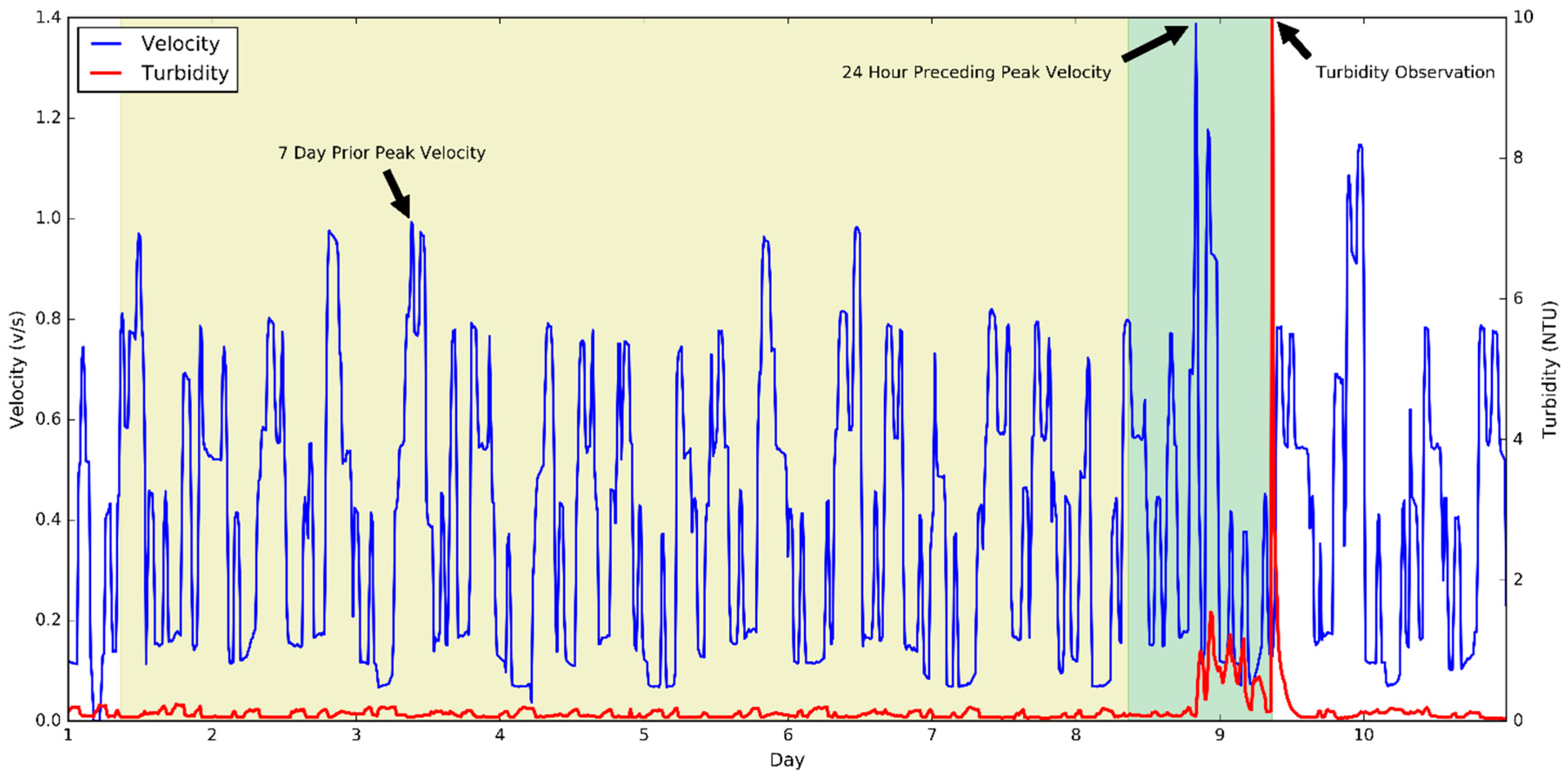
An example of the methodology is shown in Figure 1 where velocity and turbidity observations from a real trunk main system are displayed. For the sake of brevity, the methodology is visualised for a single turbidity observation and for which the peak turbidity observation is chosen. The length of time set for y is 24 h because it was sufficiently long enough for all potentially mobilised material from the furthest upstream point to reach the downstream turbidity meter. The length of time set for x is 7 days and was chosen solely for the ease of visualizing this example.
The velocity profile 24 h preceding the turbidity observation (highlighted green) is where the peak mobilising velocity is calculated. The 7 days prior (highlighted yellow) is where the preconditioned velocity threshold is calculated. The peak mobilising velocity (i.e., ) of this upstream pipe is greater than its preconditioned velocity threshold (i.e., ), and thus, the turbidity observation is determined to have resulted from the hydraulic mobilisation of discolouration material in this pipe.
From the velocity and turbidity measurements shown in Figure 1, it can also be seen that the velocity just before the start of Day 10 also exceeds the peak velocity indicated on Day 3. However, no subsequent turbidity response is seen on Day 10 because that pipe is now reconditioned to the new preconditioned velocity threshold at the end of Day 8 (i.e., all discolouration material that could have been mobilised by this new velocity was already mobilised by the peak velocity at the end of Day 8).
2.1. Chi-Square Test for Independence
While the high turbidity observation examined in Figure 1 is determined to have been caused by the hydraulic mobilisation of discolouration material, it is possible that the velocity profile and preceding turbidity response were coincidental. Thus, the chi-square test for independence will be used to determine the statistical significance of the results.
All turbidity observations will be divided into two turbidity sets of over 1 NTU observations and under 1 NTU observation, and then, each set of turbidity observations will be examined separately. HMTP>1NTU will show the percentage of turbidity observations above 1 NTU that are deemed to be caused by hydraulic mobilisation, and likewise, HMTP<1NTU will show the percentage of turbidity observations below 1 NTU that are deemed to be caused by hydraulic mobilisation. The turbidity threshold of 1 NTU was chosen as it is a clear quantifiable response above background turbidity levels and is the U.K. regulatory limit for water leaving water treatment works [27]. Therefore, a turbidity observation over 1 NTU can be considered as part of a turbidity event, and turbidity observations under 1 NTU can be considered as the absence of a turbidity event.
The proposed null hypothesis is that the turbidity level (i.e., over 1 NTU or under 1 NTU) is independent of an upstream pipe’s preceding peak velocity that exceeds the preconditioned velocity threshold. The proposed alternative hypothesis is that higher turbidity levels (i.e., over 1 NTU) are dependent on an upstream pipe’s preceding peak velocity that exceeds the preconditioned velocity threshold. Thus, for a statistically-significant result where the null hypothesis can be rejected, a HMTP>1NTU significantly greater than a corresponding HMTP<1NTU is expected to be seen.
The significance level chosen is 0.01, and the chi-square test statistic with 1 degree of freedom is used to calculate the statistical significance.
2.2. Pipes and Pipes in Series
The methodology examines each pipe upstream of the turbidity meter, where a pipe is determined here by stretches of piping where the velocity remains the same. This means an import and export branch or change in diameter determines the boundaries of a pipe.
While each pipe can be examined individually to estimate the amount of discolouration material linked to that pipe, the preconditioned velocity threshold of multiple pipes can be simultaneously exceeded and discolouration material mobilised from multiple pipe simultaneously. This would mean that some turbidity observations are counted as originating from more than one pipe.
Thus, to accurately assess the total amount of turbidity observations that can be linked to hydraulic mobilisation, all pipes upstream of the turbidity meter are also jointly assessed. This is done by separately assessing if any pipe upstream of the turbidity meter experienced a velocity that exceeded their preconditioning velocity threshold. The multiple pipes that are jointly assessed will be called pipe sets.
3. Case Studies
3.1. Description of Sites
Flow and turbidity measurements were taken over two years and 11 months from three hydraulically distinct parts of a real Water Resource Zone (WRZ) in the U.K., starting from 1 September 2013 until 1 August 2016. The three sites range from 6 km to 23 km in network length, 300 mm to 700 mm in pipe diameter size and are each primarily comprised of Ductile Iron (DI). While Site 1 has two turbidity meters, Sites 2 and 3 both have only a single turbidity meter. All turbidity meters were placed at the downstream end of each site, just upstream of a flow meter so that each turbidity measurement has an associated flow measurement. Except for a few insignificantly small water consumptions taken directly off some trunk mains, every inlet and outlet of each site was hydraulically metered by a flow meter.
Site 1 is a trunk main network with one import and six exports. Aside from a flow meter placed directly after the upstream service reservoir, which is the sole inlet for the trunk main network, the other six flow meters were each placed at an exporting branch. Site 1 can be broken down into six pipes and denoted as A, B, C, D, E, F. Pipes A, B, C, D are located upstream of Turbidity Meter (TM) A, and pipes A, B, E, F are located upstream of TM B.
Site 2 is a 6.5 km trunk main with one import and two exports. The flow velocity in this trunk main is primarily determined by two pumps at the downstream end of the main. Site 2 can be broken down into two pipes that are upstream of TM C and will be denoted as Pipes G and H.
Unlike Sites 1 and 2, Site 3 has two flow imports from two different water sources. Site 3 can be broken down into three pipes that are upstream of TM D and will be denoted as I, J and K. As the water from the further downstream import between Pipes J and K is less expensive, only a small flow is typically seen across the almost 20 km length of Pipes I and J. However, when the downstream reservoir is low on water, the upstream pumps engage to supply additional water. A schematic of Site 3 is shown in Figure 2.
A summary of each pipe upstream of each turbidity meter is shown in Table 1.
3.2. Flow and Turbidity Data
The flow and turbidity observations were logged at 15-min intervals with flow recorded as the sum of water through the meter during that interval and turbidity observations recorded as the current turbidity value at the interval. Flow was originally recorded in cubic meters per 15 min (m3/15 min) and turbidity in NTU. A summary of the turbidity data for each turbidity meter is shown in Table 2.
While all turbidity meters captured data over the same time period, TM D in Site 3 was offline for a total of six months, from July 2014 to November 2014 and then from June 2016 to August 2016. This is a considerable factor in why TM D has fewer turbidity observations over 1 NTU than the other turbidity meters. As shown by the 99th percentiles in Table 2, the vast majority of turbidity observations are significantly less than the 1 NTU threshold chosen in the methodology.
4. Results
4.1. Hydraulically Mobilised Turbidity Percentage
The results of the HMTP using an x of 1 day and y of 1 day applied to each turbidity meter and its corresponding jointly assessed pipe set are shown in Table 3.
A length of 1 day was chosen for the y parameter because it was sufficiently long enough for material mobilised from the furthest upstream points of each site to reach their respective downstream turbidity meters. The x parameter was set to 1 day to show the maximum amount of turbidity in each site that can be linked to preceding upstream hydraulic events.
The HMTP>1NTU results in Table 3 range from 84% to 100%, thus showing that the majority of turbidity can be linked to preceding hydraulic events. However, because the requirements for the methodology to determine if there were a hydraulic event preceding a turbidity observation are quite low with only an x of 1 day (i.e., the peak velocity in the previous 24 h exceeds the prior 24-h peak velocity), the HMTP<1NTU results in Table 3 are also substantially high. While the p-values show that the null hypothesis can be rejected at a 0.01 level of significance, a significantly larger gap between the HMTP<1NTU and HMTP>1NTU results would indicate greater confidence in the methodology and results.
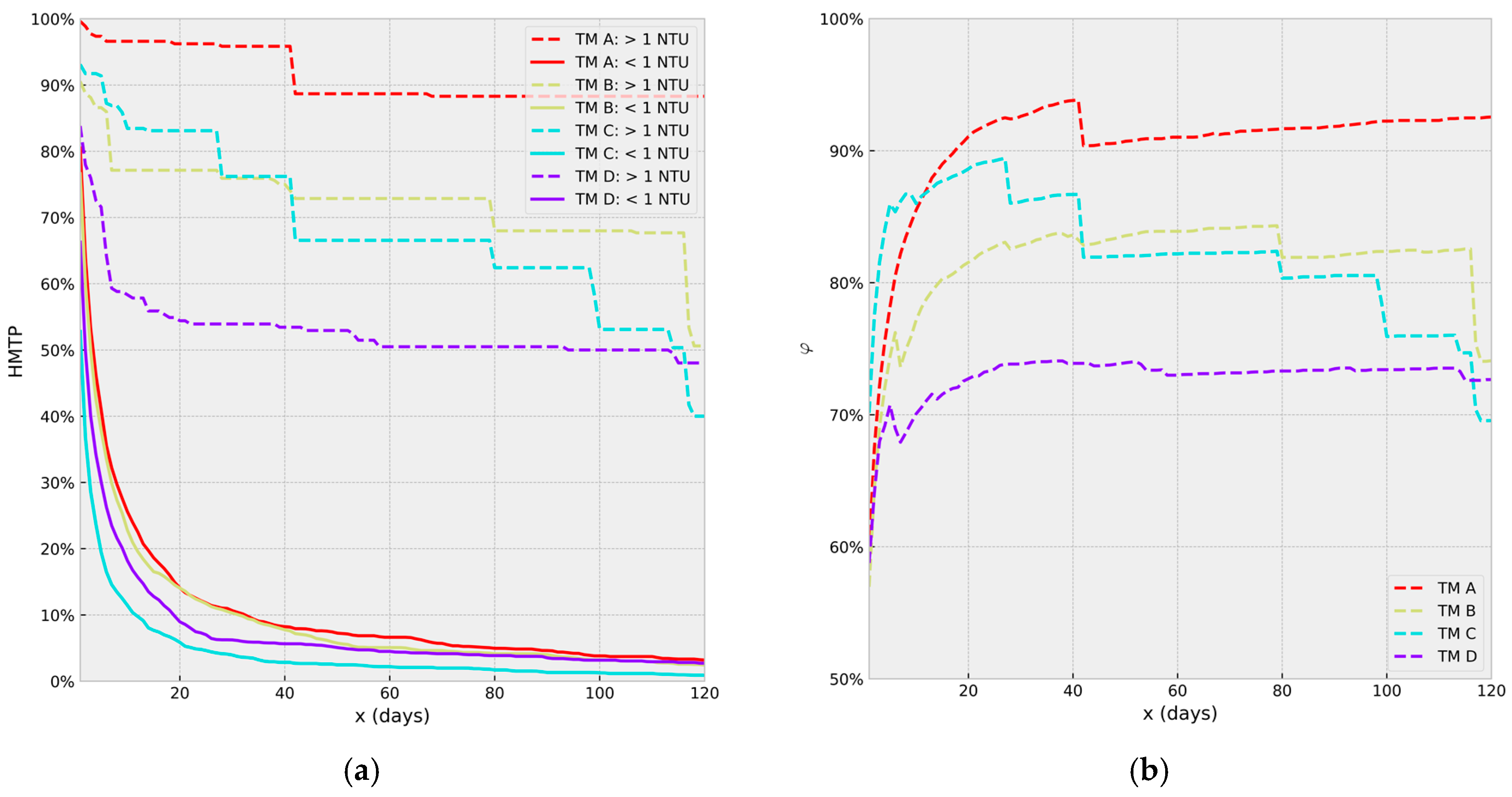
The effect of increasing the x parameter for HMTP<1NTU and HMTP>1NTU can be seen as plotted in Figure 3a. Figure 3a shows that the HMTP<1NTU of each TM exponentially decays while the HMTP>1NTU decreases at a substantially slower rate. An objective function calculating the trade-off between the HMTP<1NTU and HMTP>1NTU is given by the formula shown below:
Figure 3b shows plotted for each TM over increasing values of x. A higher indicates a better trade-off between a low HMTP<1NTU and a high HMTP>1NTU.
From the results shown in Figure 3b, a 30-day length was chosen for x, and the corresponding results for each jointly assessed pipe set followed by the results for each individual pipe that makes up that pipe set are shown in Table 4. The percentage of turbidity observations under 1 NTU that the methodology deemed to be hydraulically mobilised ranges from 3% to 5% for individual pipes and 4% to 11% for the grouped pipe sets; while the percentage of turbidity observations over 1 NTU ranges from 0% to 84% for individual pipes and 54% to 96% for the grouped pipe sets.
Note that the sum of HMTP>1NTU for individual pipes belonging to each turbidity meter exceeds 100%. This was expected because, as mentioned above, a turbidity observation can be linked to multiple pipes if a hydraulic event occurs in both pipes simultaneously.
For the results of TM A, a high HMTP>1NTU of 84% is given for Pipe C. This is important to note because as can be seen from Table 1, Pipe C had a low 99th velocity percentile of 0.17 m/s, which indicates a high potential for material build up. The 12% difference between the HMTP>1NTU of 84% for Pipe C and the HMTP>1NTU of 96% for the pipe set is assumed to come from Pipes A and B and not Pipe D because Pipes C and D have very similar velocity profiles (when compared to Pipes A and B).
Comparing the TM A and TM B cases shows two very different sets of HMTP>1NTU results for Pipes A and B, even though they are both located on the same site. This indicates that significant discolouration material is being mobilised from Pipes A and B; and the material that travels towards TM B reaches it, but a portion of the material that travels towards TM A ends up settling/attaching in Pipe C and then remobilises at a later time.
4.2. Turbidity and Velocity Relationships
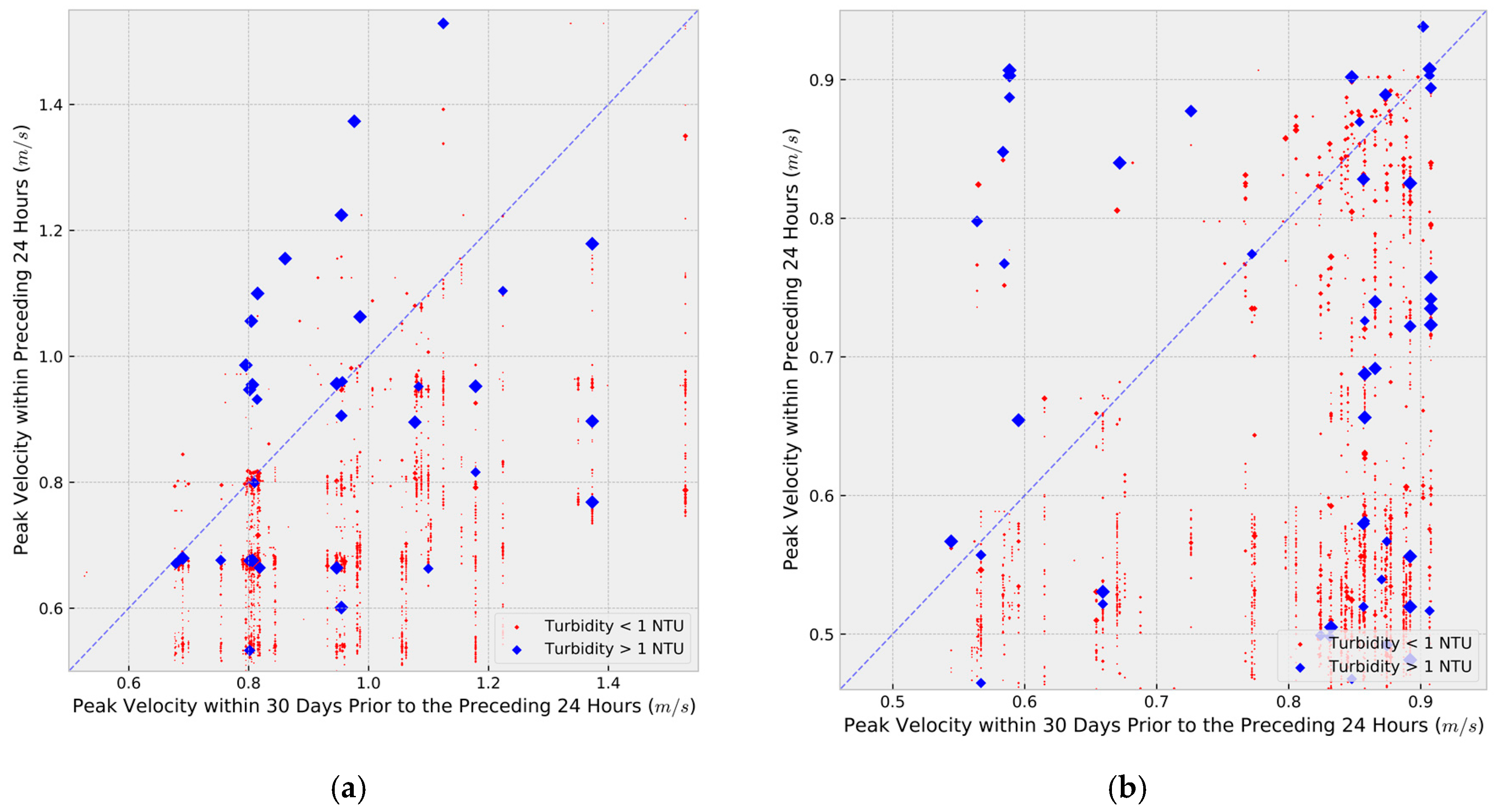
Figure 4 shows the peak velocity in the 24 h preceding a turbidity observation plotted against the peak velocity in the 30 days prior to the 24 h preceding the turbidity observation for two pipes that had the highest HMTP>1NTU for their respective turbidity meters as shown in Table 4. The size of each data point in a plot is relative to the turbidity measurement where a higher turbidity value results in a bigger data point. Because all turbidity observations from the same turbidity event should have the same 24-h preceding peak velocity and prior 30-day peak velocity, each visible data point is actually an individual turbidity event with the size of the data point representing the biggest single turbidity observation seen during that turbidity event.
The dashed line, which is also the identity line, shows where the preconditioned velocity threshold for data points along the y axis is. Hence, data points above the identity line are considered to have exceeded their preconditioned velocity thresholds for that pipe because they have experienced a velocity in the preceding 24 h that is higher than all velocities experienced in the prior 30 days. Although data points below the identity line of a specific pipe cannot be linked to hydraulic mobilisation from that pipe, it does not mean that they cannot be linked to hydraulic mobilisation from a different pipe upstream of the turbidity meter.
If a cleaning velocity (i.e., velocity at which all material is removed from pipe) existed in the any pipes, a significant number of low and only low turbidity observations would be seen above the identity line after a sufficiently high prior peak velocity (i.e., the x axis of Figure 4). However, this is not observed in any pipes, and thus, no clear mobilisation limit is seen. Similarly, by looking at only the peak velocities in pipes during the 24 h preceding the arrival of turbidity (i.e., y axis of Figure 4), a clear minimum mobilising velocity was not seen in any pipes. Instead, it can be clearly seen that turbidity observations under 1 NTU are ubiquitously present below the identity line, but not above.
Table 5 shows Spearman’s rank correlation coefficients for three different sets of velocity calculations correlated with their associated turbidity sets. Spearman’s rank correlation coefficient measures the dependence of two parameters as described as a monotonic function. Linearity between the two parameters is not assumed in Spearman correlation, which is not the case for Pearson’s correlation coefficient. A Spearman correlation coefficient of 1 or −1 indicates a perfect monotonic relationship. For each correlation coefficient, an associated p-value is derived from a statistical t-test, which indicates the probability of an uncorrelated system generating datasets that have a correlation at least as extreme.
The first correlation is the 24h Peak Velocity which is the 24-h preceding peak velocities of each turbidity observation, regardless of turbidity value, correlated with those turbidity observations. The very weak to weak positive correlation across all pipes shows that higher preceding velocities alone rarely indicate the appearance of higher turbidity concentrations downstream. However, these correlations are predominantly driven by the many low bulk flow turbidity observations and tell little about the correlation between peak velocities preceding a turbidity event and the amount of turbidity mobilised in that event. Thus, the second correlation set shown in Table 5 is the 24-h Peak Event Velocity where the 24-h preceding peak velocities of turbidity events are correlated with the downstream turbidity observations of those turbidity events. Interestingly, there are a few negative correlations, but because they are very weak correlations, not much can be inferred.
The third correlation set is the Exceeded Velocity Difference where the difference between the 24-h preceding peak velocity and the 30-day preconditioned velocity threshold (i.e., the identity lines shown in Figure 4) of each turbidity event is correlated with the turbidity observations of those events. While the largest correlation is only 0.55, the majority of correlations are moderately positive, which is significantly stronger compared to the 24-h Peak Velocity and 24-h Peak Event Velocity correlations. This shows that the exceeded velocity difference is a better indicator of the resulting turbidity event size than a preceding increase in velocity alone.
5. Discussion
A sum total of 1087 turbidity observations of over 1 NTU were recorded from just under three years’ worth of turbidity measurements at four turbidity meters. As each observation is taken at a 15-min interval, this is equivalent to using 54 turbidity events where the turbidity level of each event is at least 1 NTU for over 5 h straight. When considering that turbidity is akin to a concentration and is significantly diluted by the high flow rates typical of trunk mains, then even relatively low turbidity observations in trunk mains should be of somewhat concern. This is because the discoloration material that does not directly reach a customer’s tap can still resettle in a downstream network. Then, that same discolouration material when remobilised in a smaller distribution pipe with a fraction of the flow rate could result in a significantly higher turbidity reading.
Discolouration material clearly does build up in the trunk mains observed in this paper, this is despite the relatively high velocity percentiles shown in Table 1 that vastly exceed the ‘self-cleaning’ velocity ranges (0.25 m/s–0.4 m/s) associated with smaller distribution pipes [3,28]. This agrees with the findings of other authors conducted on large diameter pipes (i.e., over 200 mm), which find no evidence for self-cleaning velocities or shear stresses [18,24,29].
The majority of p-values in Table 3 and Table 4 show the null hypothesis being overwhelmingly rejected at a 0.01 level of significance and thus conclude that higher turbidity levels (i.e., over 1 NTU) can be explained by an upstream pipe’s preceding peak velocity exceeding its preconditioned velocity threshold. These p-values here are particularly low due to the high number of turbidity observations considered (i.e., over 100,000), thus making it very unlikely that these values would be seen in uncorrelated results.
The only exceptions in results seen in Table 4 and Table 5 are Pipes E and F for TM B, which are distinctly different from all other results as, conversely, only a few high turbidity observations can be linked to preceding hydraulic events in these pipes. This may be indicative of an underlying process that is either preventing discolouration material from sufficiently accumulating in these pipes or the methodology from accurately modelling them.
Important to note is that the velocity peaks preceding turbidity observations are a relatively small increase in comparison to the average daily peak velocity, typically being less than 110% of the average daily peak velocity. This shows how sensitive discolouration material can be to mobilising velocities and indicates why discolouration is so often attributed to scheduled works that alter velocities in WDS.
While Table 3 shows that a maximum amount of 84% to 100% of turbidity observations over 1 NTU in the trunk mains examined here can be linked to hydraulic mobilisation, this also conversely shows that between 0% and 16% of turbidity observations cannot be linked to the hydraulically-driven mobilisation process outlined in this paper. This leaves a few possibilities about the mobilisation of the remaining turbidity: (a) some of the discolouration material was mobilised from further upstream (i.e., reservoirs or treatment works); (b) a hydraulic process not accounting for such as a transient event or flow reversal caused some mobilisation; (c) a non-hydraulic process caused some mobilisation (e.g., biofilm detachment/sloughing that can sometimes occur without an increase in hydraulic force).
The methodology presented here does not make any assumptions about what the discolouration material consists of (e.g., manganese, biofilms), what form the discolouration material takes inside pipes (e.g., sediment, cohesive layers), nor does it assume a rate (e.g., linear, exponential) at which discolouration material is mobilised. Additionally, because the mobilisation condition has been reduced to a simple “greater than prior” condition, as long as the hydraulic force has a monotonic relationship to the flow rate, it also does not matter what the hydraulic force is (e.g., velocity, shear stress, laminar boundary layer size). This means, in theory, that the methodology could be applied to almost any WDS regardless of the material composition, layout and range of flow rates of the WDS.
As flow meters are already ubiquitous in WDS, this methodology also shows the potential information gain from installing even a single turbidity meter. As the accuracy of the methodology to identify the primary sources of discolouration increases with more data, installing a turbidity meter at a downstream service reservoir where regular maintenance is easily achievable is advised. If possible, further turbidity meters should be installed at the downstream ends of different network branches. This would enable the correlation of methodology results to further identify high discolouration risk pipes, as was shown done for Site 1.
Regarding the frequency of flow and turbidity observations, while a 15 min sampling frequency was deemed sufficient for the sites examined here, a higher frequency may be required for WDSs that can experience sharp, but short-lived velocity spikes. This is because a significant, but short-lived velocity spike that could cause discolouration may only present as a minor increase in the cumulative flow over a 15 min period.
6. Conclusions
This paper presents a long-term continuous study of discolouration mobilisation and a methodology to determine the approximate amount and origin of hydraulically mobilised turbidity in trunk mains. The methodology is validated on three real sites in the U.K. The following conclusions are made based on the case studies results obtained:
- (a)
- The methodology shows that for the four turbidity meters used in this study, a maximum of 84%, 91%, 93% and 100% of turbidity observations over 1 NTU could be linked to preceding hydraulic forces that exceeded an upstream pipe’s hydraulically preconditioned state. This shows that the mobilisation of discolouration material is predominantly determined by hydraulic forces, which, in turn, indicates significant potential for modelling and predicting discolouration events.
- (b)
- The methodology showed that even without a calibrated hydraulic model, it is possible to determine the approximate origin of discolouration material that had been hydraulically mobilised within each site analysed. This can be used as an aid in the prioritisation of cleaning trunk mains and targeted mains rehabilitation.
- (c)
- The level of turbidity is shown to be significantly dependent on preceding upstream velocities that exceed a pipe’s preconditioned state. Furthermore, discolouration material is shown to accumulate regardless of the velocity magnitude, thus indicating that controlling the shape of the hydraulic profile is vital in effectively managing discolouration risk.
Acknowledgments
The authors are grateful to the Engineering and Physical Sciences Research Council (EPSRC) for providing the financial support as part of the STREAM project and to Julian Collingbourne of South West Water for supplying the data used in this paper.
Author Contributions
Each of the authors contributed to the design, analysis and writing of the study.
Conflicts of Interest
The authors declare no conflict of interest.
References
- OFWAT Serviceability Outputs for PR09 Final Determinations. Available online: https://www.ofwat.gov.uk/wp-content/uploads/2015/11/det_pr09_finalfull.pdf (accessed on 22 August 2017).
- DWI Drinking Water Quality Events in 2013. Available online: http://dwi.defra.gov.uk/about/annual-report/2013/dw-events.pdf (accessed on 22 August 2017).
- Vreeburg, I.J.H.G.; Boxall, D.J.B. Discolouration in potable water distribution systems: A review. Water Res. 2007, 41, 519–529. [Google Scholar] [CrossRef] [PubMed]
- Armand, H.; Stoianov, I.I.; Graham, N.J.D. A holistic assessment of discolouration processes in water distribution networks. Urban Water J. 2017, 14, 263–277. [Google Scholar] [CrossRef]
- Douterelo, I.; Boxall, J.B.; Deines, P.; Sekar, R.; Fish, K.E.; Biggs, C.A. Methodological approaches for studying the microbial ecology of drinking water distribution systems. Water Res. 2014, 65, 134–156. [Google Scholar] [CrossRef] [PubMed]
- Vreeburg, J.H.G.; Schippers, D.; Verberk, J.Q.J.C.; van Dijk, J.C. Impact of particles on sediment accumulation in a drinking water distribution system. Water Res. 2008, 42, 4233–4242. [Google Scholar] [CrossRef] [PubMed]
- Liu, G.; Zhang, Y.; Knibbe, W.-J.; Feng, C.; Liu, W.; Medema, G.; van der Meer, W. Potential impacts of changing supply-water quality on drinking water distribution: A review. Water Res. 2017, 116, 135–148. [Google Scholar] [CrossRef] [PubMed]
- Makris, K.C.; Andra, S.S.; Botsaris, G. Pipe scales and biofilms in drinking-water distribution systems: Undermining finished water quality. Crit. Rev. Environ. Sci. Technol. 2014, 44, 1477–1523. [Google Scholar] [CrossRef]
- Fish, K.; Osborn, A.M.; Boxall, J.B. Biofilm structures (EPS and bacterial communities) in drinking water distribution systems are conditioned by hydraulics and influence discolouration. Sci. Total Environ. 2017, 593–594, 571–580. [Google Scholar] [CrossRef] [PubMed]
- Husband, S.; Boxall, J.B. Field studies of discoloration in water distribution systems: Model verification and practical implications. J. Environ. Eng. 2009, 136, 86–94. [Google Scholar] [CrossRef]
- Husband, P.S.; Whitehead, J.; Boxall, J.B. The role of trunk mains in discolouration. Proc. Inst. Civ. Eng. Water Manag. 2010, 163, 397–406. [Google Scholar] [CrossRef]
- Armand, H.; Stoianov, I.; Graham, N. Investigating the impact of sectorized networks on discoloration. Procedia Eng. 2015, 119, 407–415. [Google Scholar] [CrossRef]
- Blokker, E.J.M.; Schaap, P.G. Temperature influences discolouration risk. Procedia Eng. 2015, 119, 280–289. [Google Scholar] [CrossRef]
- Cook, D.M.; Boxall, J.B. Discoloration material accumulation in water distribution systems. J. Pipeline Syst. Eng. Pract. 2011, 2, 113–122. [Google Scholar] [CrossRef]
- Cook, D.M.; Husband, P.S.; Boxall, J.B. Operational management of trunk main discolouration risk. Urban Water J. 2015, 13, 382–395. [Google Scholar] [CrossRef]
- Husband, S.; Boxall, J. Understanding and managing discolouration risk in trunk mains. Water Res. 2016, 107, 127–140. [Google Scholar] [CrossRef] [PubMed]
- Sunny, I.; Husband, S.; Drake, N.; Mckenzie, K.; Boxall, J. Quantity and quality benefits of in-service invasive cleaning of trunk mains. Drink. Water Eng. Sci. Discuss. 2017, 1–9. [Google Scholar] [CrossRef]
- Vreeburg, J.H.G.; Beverloo, H. Sediment accumulation in drinking water trunk mains. In Proceedings of the 11th International Conference on Computing and Control for the Water Industry, Urban Water Management: Challenges and Opportunities, Exeter, UK, 5–7 September 2011. [Google Scholar]
- Boxall, J.B.; Saul, A.J. Modeling discoloration in potable water distribution systems. J. Environ. Eng. 2005, 131, 716–725. [Google Scholar] [CrossRef]
- Verberk, J.; Hamilton, L.A.; O’Halloran, K.J.; Van Der Horst, W.; Vreeburg, J. Analysis of particle numbers, size and composition in drinking water transportation pipelines: Results of online measurements. Water Sci. Technol. Water Supply 2006, 6, 35–43. [Google Scholar] [CrossRef]
- Meyers, G.; Kapelan, Z.; Keedwell, E.; Randall-Smith, M. Short-term forecasting of turbidity in a UK water distribution system. Procedia Eng. 2016, 154, 1140–1147. [Google Scholar] [CrossRef]
- Meyers, G.; Kapelan, Z.; Keedwell, E. Short-term forecasting of turbidity in trunk main networks. Water Res. 2017, 124, 67–76. [Google Scholar] [CrossRef] [PubMed]
- Gaffney, J.W.; Boult, S. Need for and use of high-resolution turbidity monitoring in managing discoloration in distribution. J. Environ. Eng. 2012, 138, 637–644. [Google Scholar] [CrossRef]
- Husband, P.S.; Jackson, M.; Boxall, J.B. Trunk main discolouration trials and strategic planning. In Proceedings of the 11th International Conference on Computing and Control for the Water Industry, Urban Water Management: Challenges and Opportunities, Exeter, UK, 5–7 September 2011. [Google Scholar]
- Slaats, P.G.G.; Rosenthal, L.P.M.; Siegers, W.G.; van den Boomen, M.; Beuken, R.H.S.; Vreeburg, J.H.G. Processes Involved in the Generation of Discolored Water; AWWA Research Foundation: Denver, CO, USA, 2003. [Google Scholar]
- Furnass, W.R.; Collins, R.P.; Husband, P.S.; Sharpe, R.L.; Mounce, S.R.; Boxall, J.B. Modelling both the continual erosion and regeneration of discolouration material in drinking water distribution systems. Water Sci. Technol. Water Supply 2014, 14, 81. [Google Scholar] [CrossRef]
- DWI Public Water Supplies in the Western Region of England. Available online: http://dwi.defra.gov.uk/about/annual-report/2014/ (accessed on 13 March 2016).
- Blokker, E.J.M.; Vreeburg, J.H.G.; Schaap, P.G.; van Dijk, J.C. The self-cleaning velocity in practice. In Proceedings of the Water Distribution System Analysis Conference, Tucson, AZ, USA, 12–15 September 2010. [Google Scholar]
- Seth, A.D.; Husband, P.S.; Boxall, J.B. Rivelin trunk main flow test. In Proceedings of the 10th International on Computing and Control for the Water Industry, Sheffield, UK, 1–3 September 2009; Maksimovic, B., Ed.; Taylor Francis: Oxfordshire, UK, 2009; pp. 431–434. [Google Scholar]
Figure 1.
An example of the methodology showing that the turbidity observation could be linked to the preceding upstream hydraulic mobilisation of discolouration material. The 24 h preceding the turbidity observation are highlighted green, and the 7 prior days are highlighted yellow. The preceding 24-h peak velocity is shown to be the cause of the high turbidity observation as it exceeds the prior 7-day peak velocity. NTU: Nephelometric Turbidity Units.

Figure 2.
Schematic of Site 3. DMA, District Metered Area.
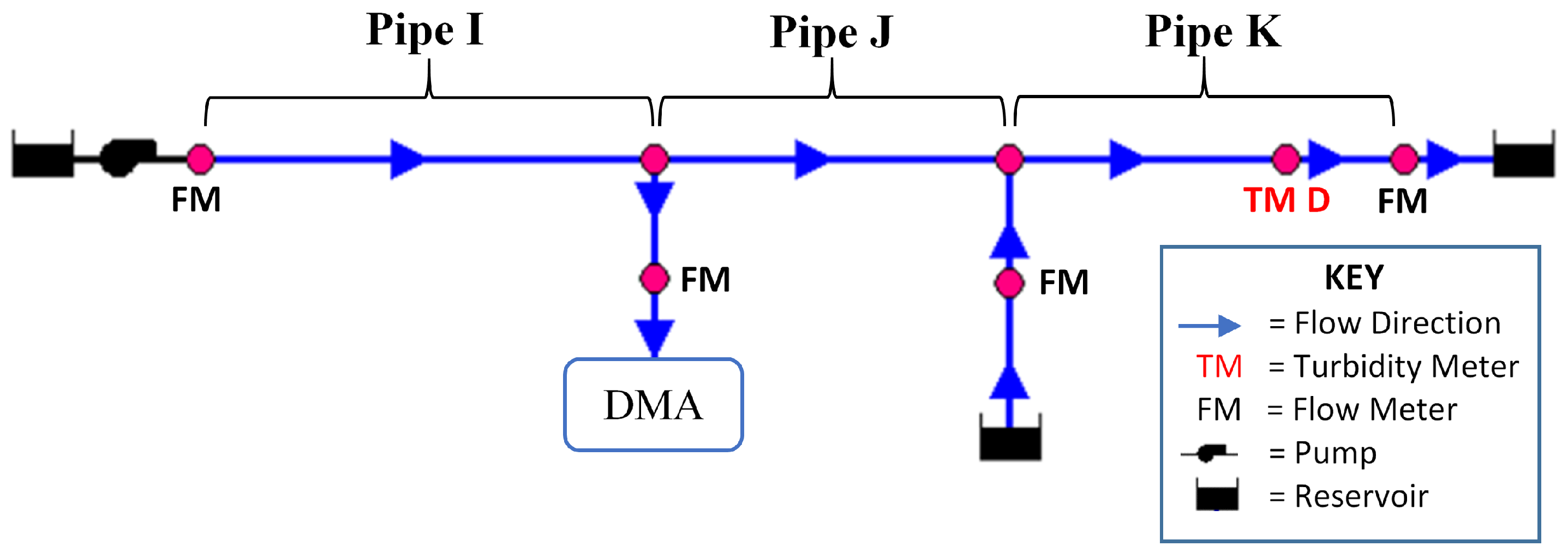
Figure 3.
(a) The HMTP<1NTU and HMTP>1NTU are shown for each TM over increasing x parameters; (b) the objective formula φ is shown for each TM over increasing x parameters.
Figure 3.
(a) The HMTP<1NTU and HMTP>1NTU are shown for each TM over increasing x parameters; (b) the objective formula φ is shown for each TM over increasing x parameters.

Figure 4.
For each turbidity observation, the 24-h preceding peak velocity was plotted against the peak velocity of the 30 days prior to the 24 h preceding the turbidity observation. (a) Site 2, Turbidity Meter C, Pipe H; (b) Site 3, Turbidity Meter D, Pipe K.
Figure 4.
For each turbidity observation, the 24-h preceding peak velocity was plotted against the peak velocity of the 30 days prior to the 24 h preceding the turbidity observation. (a) Site 2, Turbidity Meter C, Pipe H; (b) Site 3, Turbidity Meter D, Pipe K.

Table 1.
Pipe characteristics and the 99th velocity percentile over all observed data for each site.
Table 1.
Pipe characteristics and the 99th velocity percentile over all observed data for each site.
| Site | Pipe | Length | Diameter | Upstream of Turbidity Meter | 99th Velocity Percentile |
|---|---|---|---|---|---|
| 1 | A | 1.8 km | 700 mm | A, B | 0.94 m/s |
| B | 1.6 km | 700 mm | A, B | 0.92 m/s | |
| C | 1.9 km | 600 mm | A | 0.17 m/s | |
| D | 5.1 km | 300 mm | A | 0.65 m/s | |
| E | 1.8 km | 400 mm | B | 0.86 m/s | |
| F | 4.4 km | 400 mm | B | 0.80 m/s | |
| 2 | G | 1.9 km | 450 mm | C | 0.83 m/s |
| H | 4.6 km | 450 mm | C | 0.80 m/s | |
| 3 | I | 11 km | 400 mm | D | 0.79 m/s |
| J | 8.5 km | 400 mm | D | 0.70 m/s | |
| K | 3.6 km | 400 mm | D | 0.73 m/s |
Table 2.
Summary of turbidity observations for each site.
| Turbidity Meter (TM) | Duration Monitored | 99th Percentile (NTU) | Observations >1 NTU |
|---|---|---|---|
| TM A (Site 1) | 2 years, 11 months | 0.41 | 265 |
| TM B (Site 1) | 2 years, 11 months | 0.42 | 328 |
| TM C (Site 2) | 2 years, 11 months | 0.36 | 290 |
| TM D (Site 3) | 2 years, 5 months | 0.46 | 204 |
Table 3.
Hydraulically Mobilised Turbidity Percentage (HMTP) carried out on each pipe in series between the upstream sources and downstream service reservoirs to assess the amount of turbidity observations that can be linked to hydraulic mobilisation. The x and y parameters of HMTP were set to 1 day.
| Turbidity Meter | Pipes in Set | HMTP<1NTU | HMTP>1NTU | p-Value |
|---|---|---|---|---|
| TM A (Site 1) | A, B, C, D | 81% | 100% | p < 10−9 |
| TM B (Site 1) | A, B, E, F | 77% | 91% | p ≈ 10−8 |
| TM C (Site 2) | G, H | 53% | 93% | p < 10−9 |
| TM D (Site 3) | I, J, K | 66% | 84% | p ≈ 10−6 |
Table 4.
Hydraulically Mobilised Turbidity Percentage (HMTP) results with the x parameter set to 30 days and the y parameter set to 1 day.
Table 4.
Hydraulically Mobilised Turbidity Percentage (HMTP) results with the x parameter set to 30 days and the y parameter set to 1 day.
| Turbidity Meter | Pipes | HMTP<1NTU | HMTP>1NTU | p-Value |
|---|---|---|---|---|
| TM A (Site 1) | A, B, C, D | 11% | 96% | p < 10−9 |
| A | 4% | 26% | p < 10−9 | |
| B | 4% | 33% | p < 10−9 | |
| C | 5% | 84% | p < 10−9 | |
| D | 5% | 81% | p < 10−9 | |
| TM B (Site 1) | A, B, E, F | 10% | 76% | p < 10−9 |
| A | 4% | 75% | p < 10−9 | |
| B | 4% | 75% | p < 10−9 | |
| E | 5% | 1% | p = 1 | |
| F | 5% | 0% | p = 1 | |
| TM C (Site 2) | G, H | 4% | 76% | p < 10−9 |
| G | 4% | 76% | p < 10−9 | |
| H | 3% | 76% | p < 10−9 | |
| TM D (Site 3) | I, J, K | 6% | 54% | p < 10−9 |
| I | 3% | 41% | p < 10−9 | |
| J | 3% | 39% | p < 10−9 | |
| K | 4% | 52% | p < 10−9 |
Table 5.
Spearman’s rank correlation coefficients and associated p-values for three sets of correlations: (a) 24-h preceding peak velocities of each turbidity observation correlated with those turbidity observations; (b) 24-h preceding peak velocities of each turbidity event correlated with the turbidity observations of that event; (c) the difference between the 24-h preceding peak velocity and the 30-day preconditioned threshold of each turbidity event correlated with the turbidity observations of that event.
| Turbidity Meter | Pipe | (a) 24-h Peak Vel. | p-Value | (b) 24-h Peak Event Vel. | p-Value | (c) Exceeded Vel. Difference | p-Value |
|---|---|---|---|---|---|---|---|
| TM A (Site 1) | A | 0.30 | p < 10−40 | −0.16 | p ≈ 10−23 | 0.55 | p < 10−40 |
| B | 0.28 | p < 10−40 | −0.13 | p ≈ 10−15 | 0.38 | p ≈ 10−21 | |
| C | 0.29 | p < 10−40 | 0.40 | p < 10−40 | 0.13 | p ≈ 10−08 | |
| D | 0.29 | p < 10−40 | 0.41 | p < 10−40 | 0.16 | p ≈ 10−10 | |
| TM B (Site 1) | A | 0.38 | p < 10−40 | 0.22 | p < 10−40 | 0.42 | p < 10−40 |
| B | 0.38 | p < 10−40 | 0.22 | p < 10−40 | 0.48 | p < 10−40 | |
| E | 0.06 | p < 10−40 | −0.18 | p ≈ 10−32 | −0.30 | p ≈ 10−14 | |
| F | 0.02 | p ≈ 10−10 | −0.17 | p ≈ 10−31 | −0.26 | p ≈ 10−08 | |
| TM C (Site 2) | G | 0.32 | p < 10−40 | 0.40 | p < 10−40 | 0.41 | p < 10−40 |
| H | 0.30 | p < 10−40 | 0.40 | p < 10−40 | 0.41 | p < 10−40 | |
| TM D (Site 3) | I | 0.13 | p < 10−40 | 0.15 | p ≈ 10−22 | 0.44 | p < 10−40 |
| J | 0.27 | p < 10−40 | 0.14 | p ≈ 10−20 | 0.52 | p < 10−40 | |
| K | 0.31 | p < 10−40 | 0.22 | p < 10−40 | 0.24 | p ≈ 10−20 |
© 2017 by the authors. Licensee MDPI, Basel, Switzerland. This article is an open access article distributed under the terms and conditions of the Creative Commons Attribution (CC BY) license (http://creativecommons.org/licenses/by/4.0/).
Share and Cite
MDPI and ACS Style
Meyers, G.; Kapelan, Z.; Keedwell, E. Data-Driven Study of Discolouration Material Mobilisation in Trunk Mains. Water 2017, 9, 811. https://doi.org/10.3390/w9100811
AMA Style
Meyers G, Kapelan Z, Keedwell E. Data-Driven Study of Discolouration Material Mobilisation in Trunk Mains. Water. 2017; 9(10):811. https://doi.org/10.3390/w9100811
Chicago/Turabian StyleMeyers, Gregory, Zoran Kapelan, and Edward Keedwell. 2017. "Data-Driven Study of Discolouration Material Mobilisation in Trunk Mains" Water 9, no. 10: 811. https://doi.org/10.3390/w9100811
Note that from the first issue of 2016, this journal uses article numbers instead of page numbers. See further details here.