Assessment of Water Quality Improvements Using the Hydrodynamic Simulation Approach in Regulated Cascade Reservoirs: A Case Study of Drinking Water Sources of Shenzhen, China

Abstract

Water quality safety is of critical importance in environmental improvement, particularly with respect to drinking water resources worldwide. As the main drinking water sources in Shenzhen, China, the cascade reservoirs comprising the Shiyan, Tiegang, and Xili Reservoirs are highly regulated and have experienced water quality deterioration in recent years. In this study, a three-dimensional hydrodynamic and water quality model was established using the Environmental Fluid Dynamics Code (EFDC) for the cascade reservoirs. The relationships between water quality and improvement measures were quantified and the main pollution sources for individual reservoirs were identified. Results showed that the hydrodynamic and water quality model well captured the spatial and temporal variations of water level, the permanganate concentration index (COD_Mn), and total nitrogen (TN), with high resolution in the cascade reservoirs. The correlation coefficients between simulations and observations were close to 1.00 for water levels, and over 0.50 for COD_Mn and TN concentrations. The most effective methods for water quality improvement were the reduction of the runoff load for TN and transferred water load for COD_Mn in the Shiyan Reservoir, reduction of the transferred water load in the Tiegang Reservoir, and an increase in transfer water volume, especially in the flood season, in the Xili Reservoir. Internal pollution sources also played an important role in water pollution, and thus sedimentation should be cleaned up regularly. This study is expected to provide scientific support for drinking water source protection and promote the application of hydrodynamic model in water quality management.

1. Introduction

Drinking water safety is a global issue. In China, over 400 cities have been experiencing serious water shortages, and for 110 cities these shortages have been extremely serious [1]. The total water shortage was estimated to represent nearly 30~40 billion m³ per year [2]. Moreover, water pollution threatens the drinking water source regions of cities [3]. In 2014, nearly 1.3 billion tons of drinking water from 329 investigated cities were polluted, and tens of millions of residents were affected [4]. The water resource shortages and pollution seriously restricted the sustainable development of social economy, and affected the human health and safety [5,6,7,8]. Water resource saving and exploration, as well as environment protection, are critical and imminent tasks for drinking water safety in cities.

Numerical models are widely used in water quantity and quality management due to their advantages in comparative efficiency, visualization of spatial information, and applications in data-scarce areas [9]. The typical model categories are hydrological models (e.g., SWAT, MIKE-SHE), hydrodynamic models (e.g., Delft 3D), and water quality models (e.g., QUAL). For water quality management, over the past few decades, water quality models have been developed and applied to quantify the water quality response of the water body to external or internal pollution loads [10,11,12,13] and to evaluate the effectiveness of various reduction measures in water environment improvement [14,15]. Nevertheless, water quality conditions not only depend on external and internal contaminant loads, but are also related to the complicated processes of transport and transformation overland and in water bodies. The processes are driven by weather conditions (e.g., precipitation, temperature, radiation, and cloud cover), hydrological or hydrodynamic conditions (e.g., runoff volume and velocity), and so on. Thus, hydro-meteorological conditions should be considered when capturing the water quality concentrations with detailed spatial and temporal resolutions according to different types of water bodies (rivers and lakes). Although hydrological models can well simulate flow regime variations and are capable of providing hydrological boundaries for water quality models, the resulting resolutions are limited. Hydrodynamics models have advantages in simulating the flow or mixing processes driving the transport of contaminants in the water quality model [16]. Thus, the integration of hydrodynamic and water quality models is efficient for water quality management, such as in emission reduction assessments and water quality restoration [17].

The Environmental Fluid Dynamics Code (EFDC), developed by John M. Hamrick in Virginia Institute of Marine Science, is representative of hydrodynamic and water quality models [18,19,20]. The EFDC is a three-dimensional surface water modeling system for the simulation of flow fields, temperature, sediment, water quality, and other factors at different spatial and temporal scales. It has been successfully applied in various water bodies, including lakes, reservoirs, estuaries, bays, and wetlands [21,22,23,24,25]. Due to the advantages of open source codes with respect to re-development, high simulation accuracy, and good stability, EFDC has become one of the most commonly used hydrodynamic and water quality models in both China and abroad. Wu and Xu [26] applied the EFDC in the Daoxiang Lake for chlorophyll-a simulation and algal bloom prediction. Zhou et al. [27] investigated the impact of the proposed Severn Barrage on the hydrodynamic and salinity processes in the Bristol Channel and Severn Estuary by using the EFDC model with the Barrage module. Arifin [28] simulated temperature profiles in Lake Ontario and explored spring thermal bar evolution using EFDC. However, most previous applications have focused on the simulations of hydrodynamics and water quality processes in a single lake or reservoir without severe regulations.

Shenzhen is a mega-city in China with over 10 million residents. A serious shortage of water resources exists due to its specific geographic position, as it has no large rivers. Moreover, excessive development through urban construction and industrialization in the past three decades has led to massive pollution problems (e.g., poor water quality and eutrophication), which has directly threatened the safety of drinking water in the city. In this study, cascade reservoirs in the northwest part of Shenzhen were selected as our study area, i.e., the Shiyan Reservoir, the Tiegang Reservoir, and the Xili Reservoir, which are also closely linked by Water Diversion Projects. The hydrological and water quality processes are highly disturbed by both the operations of cascade reservoirs and the external water diversion projects. Therefore, the integrated simulation of hydrodynamics and water quality variations is still a very complicated task in the study area. In addition, identification of the main pollution-related sources of drinking water contamination, and implementation of stricter water resource management measures are urgently required [29]. The objectives of this study were (1) to capture the complicated hydrodynamics and water quality with high spatial and temporal resolutions in the regulated cascade reservoirs, (2) to assess the impacts of different pollution sources on water quality concentrations (including transferred water in the flood and non-flood seasons, and the effects of reducing pollution load from runoff and transferred water), and (3) to identify the main pollution source of individual reservoirs. The study was expected to yield results to ensure urban drinking water safety in Shenzhen, and provide a reference for water quality assessment and protection of reservoirs (lakes).

2. Materials and Methods

2.1. Study Area

Shenzhen is a major, fast-developing city in the south of Guangdong Province, China. The total population is over 10 million, the majority of which is concentrated in the metropolitan area. The area has a subtropical oceanic climate, which is hot and rainy in summer. The annual average temperature and precipitation are 22.5 °C and 1967 mm, respectively, and over 80% of precipitation occurs in the summer.

Shenzhen is one of the cities with the greatest severity of water shortage in China, as there are no major rivers in this region and there is a huge water consumption requirement for industry and residents. Although there is a large amount of local precipitation, the available water resources are few due to the limited storage capacity of domestic rivers. The local government attached particular importance to construction of water diversion and storage projects. Large numbers of reservoirs have been constructed since the 1960s, which have provided over 80% of water resources to the whole city.

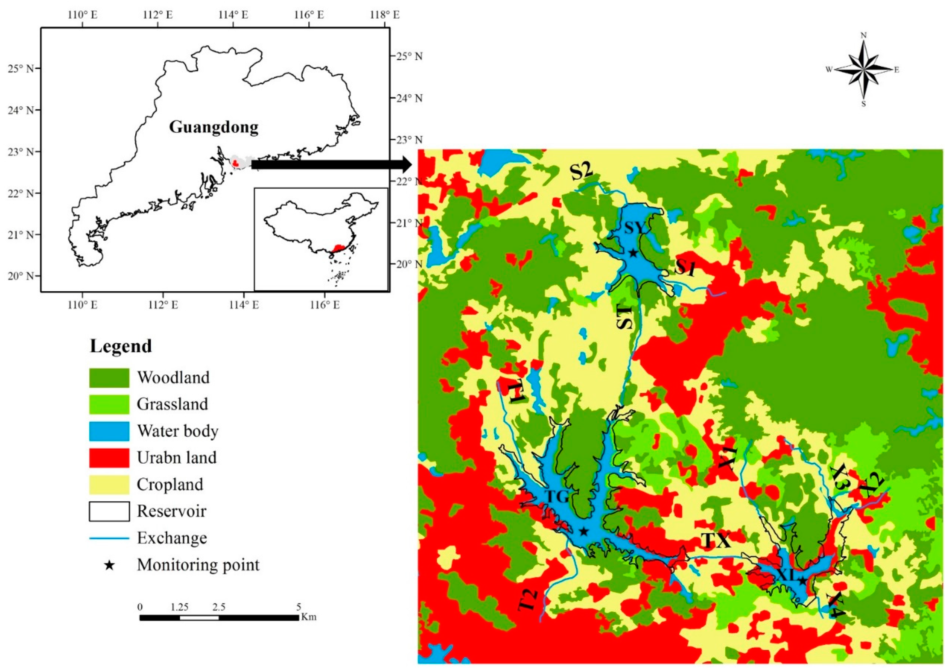
The Shiyan–Tiegang–Xili cascade reservoirs are critical projects located in the northwest of Shenzhen (113°52′–113°58′ E, 22°35′30″–22°42′30″ N) (Figure 1). These reservoirs serve as drinking water sources for the Bao’an and Nanshan districts, and as storage for water transfer and collection of urban stormwater. The maximum water storage capacity of the cascade reservoirs is over 163 million m³, accounting for nearly 40% of the total water consumption in Shenzhen. The Shiyan Reservoir, built in 1960, is located in the northwest of the cascade reservoirs. The control watershed area measures 44 km², and the total storage capacity is 32 million m³. The main tributary flowing into Shiyan Reservoir is the Shiyan River (S1). The Tiegang Reservoir, built in 1957, is located in the southwest of the cascade reservoirs, and is the biggest reservoir in Shenzhen. The control watershed area is 64 km², and the total storage capacity is 99.5 million m³. Three main tributaries flow into the Tiegang Reservoir, the Jiuwei River (T1), the Huangmabu River (T2), and the Tangtou River (T3). The Xili Reservoir, built in 1960, is located in the southeast of the cascade reservoirs. The control watershed area is 29 km² and the storage capacity is 32.39 million m³. Two main tributaries flow into the Xili Reservoir, the Baimang River (X1), and the Makan River (X3).

Flow exchanges are highly frequent among these three reservoirs. Nearly 1.20 million m³ of water is diverted to the Xili Reservoir from the East River per day through the Dongshen Water Supply Project (X2), and an average of 1.00 million m³ of water is transferred to the Tiegang Reservoir from the Xili Reservoir per day through the Connected Project (TX). The Tangtou Pumping House, as a water project (ST) taking water from Tiegang Reservoir to the Shiyan Reservoir, transfers an average of 0.7 million m³ water per day. The flow exchanges could increase water turbulence so as to increase the water self-purification capacity and improve water quality. According to the observed data in 2011, the cascade reservoirs supplied 530 million m³ of fresh drinking water, which represented 31.4% of total water supply in the whole city, and collected 28 million tons of stormwater. Thus, the water quantity and quality processes were obviously altered by a high intensity of human activity. This status directly affects the water safety in the Bao’an and Nanshan districts, and even the entire city of Shenzhen.

2.2. Data Description

Observed meteorological data, flow rate, water level data, and water quality concentrations were available for model calibration. Meteorological observation data of Shenzhen was provided from the China Meteorological Data Sharing Service System (http://cdc.cma.gov.cn/home.do) including daily atmospheric pressure, temperature, solar radiation, relative humidity, cloud cover, wind speed, wind direction, evaporation and rainfall data at meteorological stations near reservoirs. Water level and exchange flow data were provided by the Shenzhen Municipal Water Affairs Bureau. The water quality variables included the chemical oxygen demand (COD_Mn) and total nitrogen (TN). The measurements of COD_Mn and TN concentrations in the laboratory were all conducted following standard national methods [30]. Water quality data was monitored at around 10-day intervals in the cascade reservoirs, and the pollution loads of the main rivers were provided by the Shenzhen Water Quality Testing Centre.

2.3. Model Description

The EFDC was developed by John Hamrick in 1988 at the Virginia Institute of Marine Science, and is recommended by the United States Environmental Protection Agency (US EPA). The EFDC is a multifunctional surface water simulation system, which includes hydrodynamics, water quality (eutrophication), and sediment transport modules. The EFDC is one of the most widely used three-dimensional models for the simulation of flow, sediment transport, and biochemical processes in water systems. As public domain software, the model application has been reported in more than 100 water bodies all over the world, including rivers, reservoirs, lakes, estuaries, wetland and coastal seas [21,26,31,32,33,34,35].

2.3.1. Hydrodynamic Module

A physical description of hydrodynamics in EFDC is based on the Princeton Ocean Model (POM) [36]. The hydrodynamic module is based on three-dimensional hydrostatic equations formulated in curvilinear orthogonal horizontal coordinates and a sigma vertical coordinate [37]. It is a foundational module, which can simulate flow field, temperature, and salinity. It provides the hydrodynamic boundary for other modules, and at the same time, biogeochemical processes regarding the relevant water quality variables (e.g., sediment and nutrients) are calculated in the corresponding modules [38]. The momentum and continuity equations are as follows [37]:

$$\begin{array}{l}{\partial }_t(mH\mu )+{\partial }_x(m_{y}H\mu \mu )+{\partial }_y(m_{x}H\nu \mu )+{\partial }_z(m\omega \mu )-(mf+\nu {\partial }_x{m}_y-\mu {\partial }_y{m}_x)H\nu \\ =-m_{y}H{\partial }_x(g\xi +p)-m_y({\partial }_{x}h-z{\partial }_{x}H){\partial }_{z}p+{\partial }_z(m{H}^{-1}{A}_v{\partial }_z\mu )+Q_{\mu }\end{array}$$

(1)

$$\begin{array}{l}{\partial }_t(mH\nu )+{\partial }_x(m_{y}H\mu \nu )+{\partial }_y(m_{x}H\nu \nu )+{\partial }_z(m\omega \nu )-(mf+\nu {\partial }_x{m}_y-\mu {\partial }_y{m}_x)H\mu \\ =-m_{y}H{\partial }_y(g\xi +p)-m_x({\partial }_{y}h-z{\partial }_{y}H){\partial }_{z}p+{\partial }_z(m{H}^{-1}{A}_v{\partial }_z\nu )+Q_{\nu }\end{array}$$

(2)

$${\partial }_{z}p=-gH(\rho -{\rho }_0){\rho }_0{}^{-1}=-gHb$$

(3)

$${\partial }_t(m\xi )+{\partial }_x(m_{y}H\mu )+{\partial }_y(m_{x}H\nu )+{\partial }_z(m\omega )=0$$

(4)

where u and v are the horizontal velocities (m·s⁻¹) in horizontal coordinates, x and y, and are curvilinear and orthogonal, respectively; w is the vertical velocity (m·s⁻¹) in the stretched vertical coordinate z; m_x and m_y are the square roots of the diagonal components of the metric tensor, m = m_xm_y is the Jacobian of the metric tensor determinant; A_v is the vertical turbulence viscosity coefficient (m²·s⁻¹); A_b is the vertical turbulent diffusion coefficient (m²·s⁻¹); Q_u and Q_v are momentum source-sink terms; f is the Coriolis parameter; P is the physical pressure (millibar); ρ is the density (kg·m⁻³); ρ₀ is the reference density (kg·m⁻³).

2.3.2. Water Quality Module

The water quality model CE-QUAL-IC [39] is integrated into the EFDC [40]. Based on the physical conditions provided by the hydrodynamic module and the sediment–water interface behavior, the water quality module can simulate 21 state variables in water column, including four forms of algae, three forms of carbon, four forms of phosphorus, five forms of nitrogen, two forms of silica, chemical oxygen demand (COD), dissolved oxygen, and total active metal. The general governing equation for the water quality state variables is expressed as follows:

$$\begin{array}{l}{\partial }_t(m_x{m}_{y}HC)+{\partial }_x(m_{y}H\mu C)+{\partial }_y(m_{x}H\nu C)+{\partial }_z(m_x{m}_y\omega C)\\ =\frac{\partial }{\partial x}(\frac{m_{y}H{A}_x}{m_x}\frac{\partial C}{\partial x})+\frac{\partial }{\partial y}(\frac{m_{x}H{A}_y}{m_y}\frac{\partial C}{\partial y})+\frac{\partial }{\partial z}(m_x{m}_y\frac{A_z}{H}\frac{\partial C}{\partial z})+m_x{m}_{y}HSc\end{array}$$

(5)

where C is the concentration of a water quality variable (mg·L⁻¹); A_x, A_y, A_z are turbulent diffusivities in the x, y, z directions (m²·s⁻¹), respectively; Sc is the internal and external sources and sinks per unit volume; and the rest of the variables are the same as in the hydrodynamic module. In order to visualize the spatial output of water quality variables, Tecplot software [41] was adopted on the basis of source code to output simulations of all grids during the simulation.

In the EFDC model, the kinetic equation of COD is

$$\frac{\partial COD}{\partial t}=-\left(\frac{DO}{K{H}_{COD}+DO}\right)K_{COD}COD+\frac{BFCOD}{\Delta Z}+\frac{WCOD}{V}$$

(6)

where COD is the concentration of chemical oxygen demand (g O₂-equivalents·m⁻³); KH_COD is the half-saturation constant of dissolved oxygen required for oxidation of chemical oxygen demand (g O₂·m⁻³); K_COD refers to the oxidation rate of chemical oxygen demand (day⁻¹); BFCOD refers to the sediment flux of chemical oxygen demand (g O₂-equivalents·m⁻²·day⁻¹), applied to bottom layer only; WCOD refers to the external loads of chemical oxygen demand (g O₂-equivalents·day⁻¹).

The EFDC model considers five state variables for nitrogen: three organic forms (refractory particulate, labile particulate, and dissolved) and two inorganic forms (ammonium and nitrate).

$$\frac{\partial TN}{\partial t}=\frac{\partial RPON}{\partial t}+\frac{\partial LPON}{\partial t}+\frac{\partial DON}{\partial t}+\frac{\partial NH4}{\partial t}+\frac{\partial NO3}{\partial t}$$

(7)

where RPON is the concentration of refractory particulate organic nitrogen (g N·m⁻³); LPON is the concentration of labile particulate organic nitrogen (g N·m⁻³); DON is the concentration of dissolved organic nitrogen (g N·m⁻³); NH4 is the concentration of ammonium nitrogen (g N·m⁻³); NO3 is the concentration of nitrate nitrogen (g N·m⁻³).

3. Model Configuration and Calibration

3.1. Computational Domain and Grid Generation

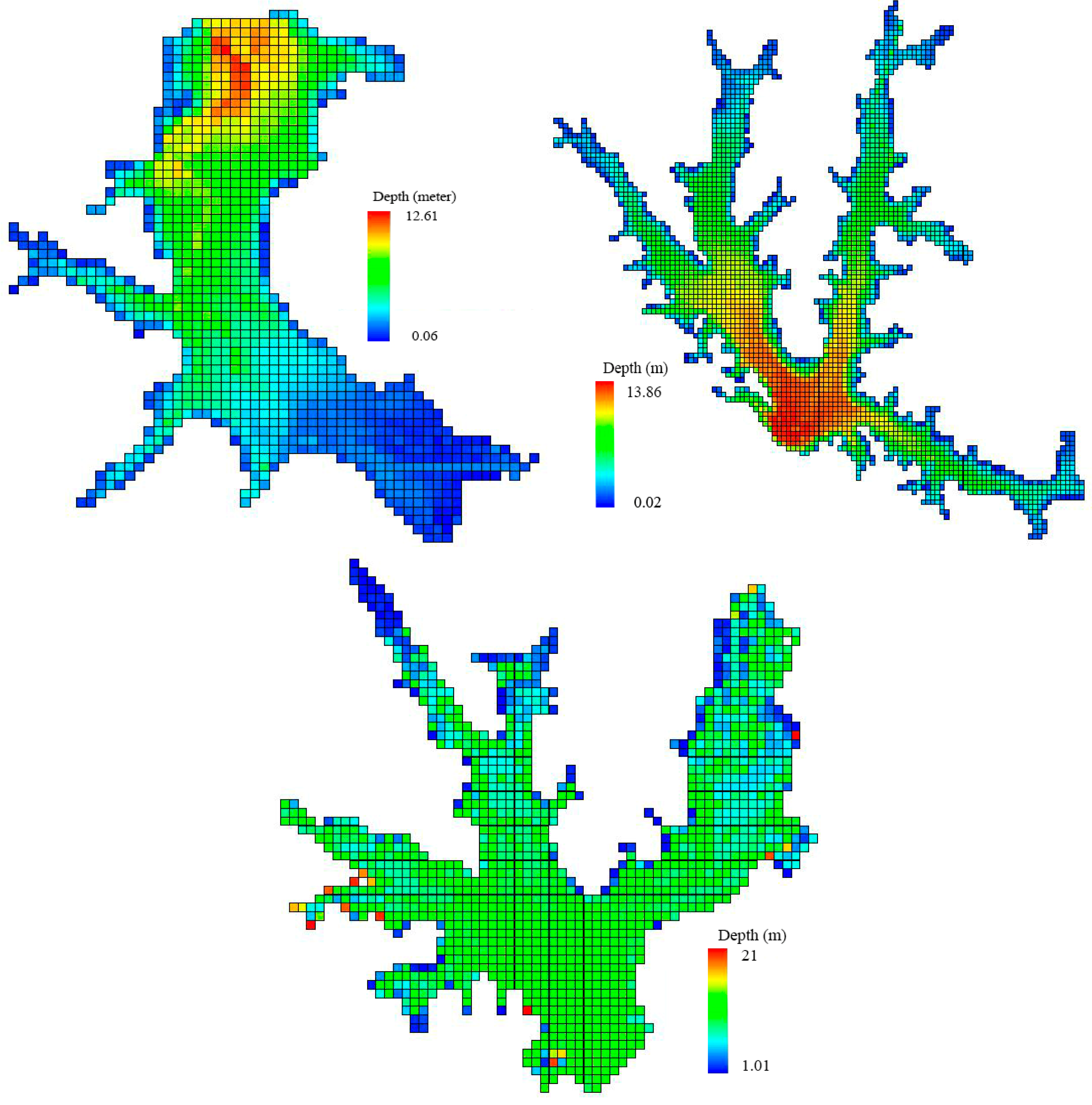
The topological and bathymetric data provided by the administration office of the reservoirs were used to generate the grid. In this study, the computational grids are at a 50 m × 50 m spatial resolution to represent the complex geometry of the cascade reservoirs. Horizontally, the final grid measures 1096 square cells in the Shiyan Reservoir, 2783 square cells in the Tiegang Reservoir, and 1344 square cells in the Xili Reservoir (Figure 2). In the vertical direction, the sigma coordinate was adopted and divided into five layers. The depth ratio of each layer was 0.2 from top to bottom.

3.2. Initial Conditions

The simulation period was from 1 January to 31 December, 2011, in which the first month was the spinning-up period. The initial conditions were set according to the observations, including water level, water temperature, flow velocity, and water quality of the cascade reservoirs (

Table 1. Initial condition of the Environmental Fluid Dynamics Code (EFDC) for the three cascade reservoirs. COD_Mn: permanganate concentration index; TN: total nitrogen.

Reservoirs	Water Level (m)	Velocity (m/s)	Temperature (°C)	CODMn (mg/L)	TN (mg/L)
Shiyan	35.40	0	14.2	2.8	2.46
Tiegang	23.05	0	14.2	2.3	1.18
Xili	27.20	0	14.2	1.35	1.42

).

3.3. Boundary Conditions

The horizontal and surface boundary conditions in the model represented external driving forces to the reservoir dynamics. The lateral boundary conditions consisted of tributary inflow rates, associated water temperature, and water quality concentrations. In the Shiyan Reservoir, the Shiyan River (S1), Ejing Reservoir transfer water, and Tiegang Reservoir transfer water (ST) were its inflows. The outflows were water supply to the water plant, transfer to other reservoirs (S2), and a spillway. In the Tiegang Reservoir, inflows included the Jiuwei River (T1), the Tangtou River (T2), the Huangmabu River (T3), and Xili Reservoir transfer water (TX). Outflows consisted of transfer water to Shiyan Reservoir (ST), water supply to the water plant, and a spillway (T4). In the Xili Reservoir, the Baimang River (X1), the Makan River (X3) and transfer water from Xijiang River (X2) were its inflows, while water supply to the water plant (X4), transfer water to Tiegang Reservoir, and a spillway were its outflows.

The surface boundary conditions were described as daily meteorological conditions, including atmospheric pressure, air temperature, relative humidity, rainfall and evaporation rate, solar short-wave radiation, cloud cover rate, wind speed, and its direction. In the modeling process, daily data were organized into a special format of EFDC to represent the meteorological boundary conditions.

3.4. Model Calibration

Hydrodynamic and water quality parameters were adjusted by a trial-and-error approach to obtain good simulation performance. The hydrodynamic parameters were calibrated first, and water quality parameters were then calibrated based on the hydrodynamic boundary provided by the hydrodynamic module. The sensitive parameters were selected according to previous studies [42] and are presented in

Table 2. Selected sensitive parameters for the hydrodynamic and water quality model. COD: chemical oxygen demand: LPON: concentration of labile particulate organic nitrogen; RPON: concentration of refractory particulate organic nitrogen; DON: dissolved organic nitrogen.

Parameter	Value	Unit
dimensionless horizontal momentum diffusivity	0.25	None
background, constant or eddy (kinematic) viscosity	1.0 × 10−7	m2·s−1
background, constant or molecular diffusivity	1.0 × 10−9	m2·s−1
reaeration rate constant	3.93	None
COD decay rate	0.10	day−1
reference temperature for COD decay	20.0	°C
minimum hydrolysis rate of RPON	0.001	day−1
minimum hydrolysis rate of LPON	0.01	day−1
minimum hydrolysis rate of DON	0.03	day−1
maximum nitrification rate	0.06	g N·m−3·day−1
benthic flux rate of ammonia nitrogen	0.01 (Shiyan)	g·m−2·day−1
	0.00 (Tiegang)
	0.08 (Xili)
benthic flux rate of chemical oxygen demand	3.00 (Shiyan)	g·m−2·day−1
	2.00 (Tiegang)
	3.00 (Xili)
benthic flux rate of nitrogen	0.50 (Shiyan)	g·m−2·day−1
	0.20 (Tiegang)
	2.00 (Xili)

. Correlation coefficient (R) and root-mean-squared-error (RMSE) were used to evaluate different parts of discrepancies between simulations and observations of water levels, concentrations of COD_Mn and TN. R was used to evaluate temporal variations between the simulations and observations, while RMSE was to evaluate the average differences between the simulation and observations. Equations (8) and (9) present the formulas for R and RMSE, respectively.

$$R={\displaystyle \sum _{i=1}^N(O_i-\overline{O})\times (S_i-\overline{S})/\sqrt{{\displaystyle \sum _{i=1}^N{(O_i-\overline{O})}^2\times {\displaystyle \sum _{i=1}^N{(S_i-\overline{S})}^2}}}}$$

(8)

$$RMSE=\sqrt{{\displaystyle \sum _{i=1}^N{(O_i-S_i)}^2/N}}$$

(9)

where O and S are the observed and simulated values, respectively; N is the number of the time series; and i is the ith of the time series. A value of 0.0 for RMSE indicates a perfect model. Moreover, in our study, if the R value is no less than 0.50 and 0.80, the simulation performances are satisfactory and good, respectively [43].

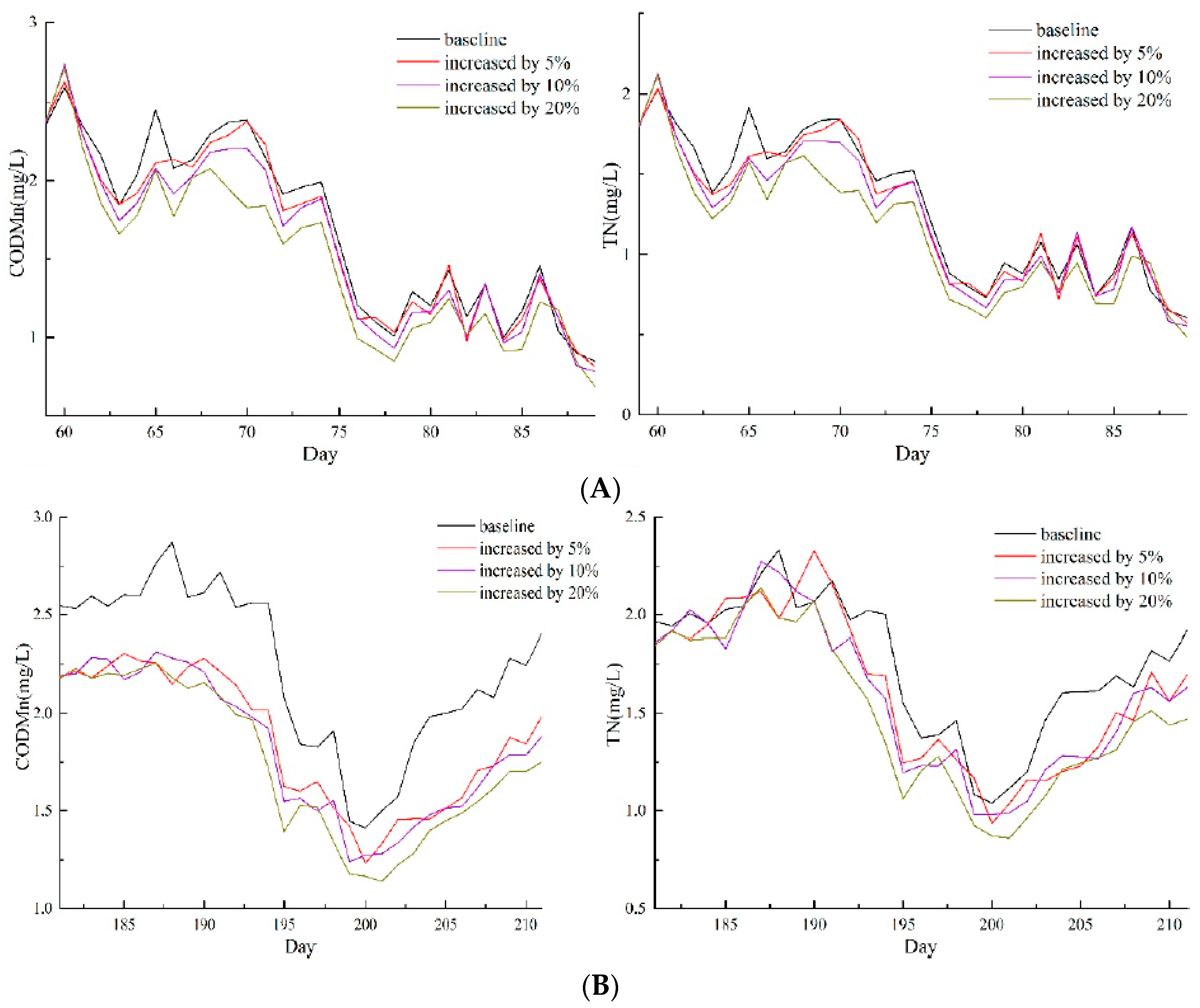
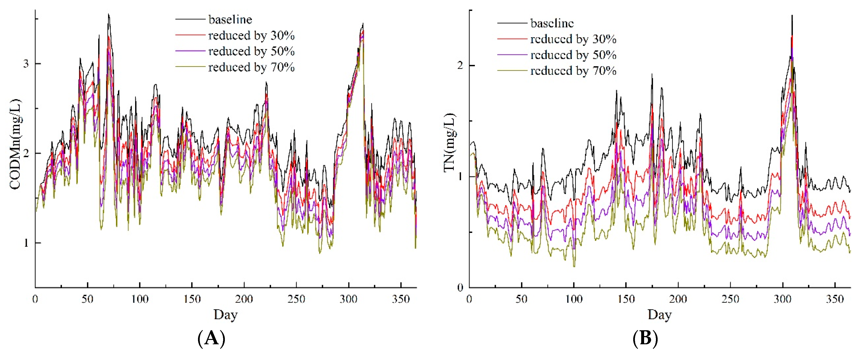
3.5. Simulation Scenarios

In this study, several scenarios were designed to explore the quantitative relationships between water quality improvement in the cascade reservoirs and the pollution load reduction or reservoir operation by the calibrated model. Reservoir operation scenarios were set to assess the impact of reservoir operation on water quantity and quality by increasing transferred water volume during flood and non-flood seasons by 5%, 10%, and 20%. In our study, March (58–89 days) and July (181–211 days) were chosen as typical months of non-flood and flood seasons, respectively. As the main pollution sources of cascade reservoirs, rainfall-runoff and transferred water had different characteristics with respect to water quantity and quality. The amount of rainfall-runoff was quite little (i.e., only 20% of inflow water), but it had very high pollutant concentrations because of industrial pollution and domestic wastewater. In contrast, owing to strict water quality management in the drinking water reservoir, the water quality conditions of transferred water were much better. Since runoff was polluted heavily, the simulated scenarios were designed to reduce COD_Mn and TN loads by 30%, 50%, and 70%, individually. The reduction ratios of COD_Mn and TN loads in the transferred water were also 30%, 50%, and 70%.

4. Results and Discussion

4.1. Hydrodynamic Calibration

Water levels in the cascade reservoirs were well simulated by the hydrodynamic module of EFDC (Figure 3). In the Shiyan Reservoir, the simulated water level was well matched with the observation, except in September. The correlation coefficient reached 0.97 and RMSE was only 0.1 m. In the Tiegang Reservoir, the correlation coefficient reached 0.997, and the RMSE was merely 0.11 m. Only the simulated water levels in the flood season were higher than in the observations. The probable reason was that the reservoir inundated the surrounding dry land in the flood season, resulting in the expansion of water area and exceeding the generalized grid area. In the Xili Reservoir, although the water level varied severely, the simulation performance was still good, i.e., the correlation coefficient reached 0.98 and RMSE was 0.1 m.

4.2. Water Quality Calibration

Figure 4 showed the simulated and observed concentrations of COD_Mn and TN in the cascade reservoirs. The overall results are summarized in

Table 3. Simulation performance of water level, COD_Mn, and TN concentrations by EFDC.

Factor	Shiyan		Tiegang		Xili
	R	RMSE	R	RMSE	R	RMSE
water level	0.97	0.10	0.997	0.11	0.98	0.10
CODMn	0.70	1.17	0.59	1.88	0.58	0.58
TN	0.60	0.76	0.51	0.28	0.27	0.61

Note: the root-mean-square error (RMSE) unit is in meters for water level, and mg/L for water quality.

for water level, COD_Mn, and TN, respectively. Due to frequent water diversion, water levels in the cascade reservoirs fluctuated dramatically, and the maximum ranges in the Tiegang Reservoir reached 5 m, which made the hydrodynamic condition complicated. As a result, the water quality simulation was much more complicated. However, the water quality model results fit the observations in cascade reservoirs quite well. The water quality model reproduced the temporal variations of COD_Mn concentrations, and R values were 0.70, 0.59, and 0.58, respectively. From June to August, the growth of phytoplankton community resulted in the decline of TN concentrations. However, in other periods, owing to the dissimilarity of inflow water with different water quality and quantity, the trend of TN was varied for each reservoir.

According to the spatial distributions of water quality in the cascade reservoirs, COD_Mn and TN concentrations showed roughly consistent distribution characteristics (Figure 5). The concentration was lower near the entrance of transfer water, and then gradually deteriorated due to the mixing action. The concentration was the highest at the area where rivers flowed into the reservoirs, because a great deal of industrial pollutant was collected along the rivers. However, according to the Chinese Environmental Quality Standards for Surface Water (GB3838-2002), the COD_Mn concentrations in most regions were of Grades II~III in the Shiyan Reservoir, and Grades I~II in the Tiegang and Xili Reservoirs, while the TN concentrations in most regions were inferior to Grade IV in all three reservoirs. Thus, eutrophication was the largest threat to the drinking water sources of these reservoirs.

4.3. Scenario Simulation and Assessment for Water Quality Improvement

4.3.1. Increase of Transferred Water Volume

Due to the increase of transferred water volume, the COD_Mn and TN concentrations reduced slightly in the center area of cascade reservoirs (

Table 4. Variation of water quality concentrations in the middle area of the cascade reservoirs under increasing different proportion transfer water (%).

Period	Factor	Shiyan			Tiegang			Xili
		5%	10%	20%	5%	10%	20%	5%	10%	20%
non-flood season	CODMn	−1.9	−3.6	−8.2	−1.5	−2.6	−5.2	−2.7	−5.7	−11.6
	TN	−3.0	−5.8	−11.0	−1.0	−1.8	−2.9	−2.9	−5.7	−12.0
flood season	CODMn	−3.8	−8.0	−14.7	−0.6	−1.4	−2.6	−16.7	−18.4	−21.8
	TN	−3.2	−7.0	−13.6	−2.3	−3.7	−6.8	−7.4	−9.3	−14.4

). In addition to COD_Mn in the Tiegang Reservoir, if the transferred water increased the same proportion, the water quality improvement was better in the flood season than in the non-flood season. In the scenario of increasing transferred water by 5%, the COD_Mn and TN concentrations were reduced by 1.5%~2.7% and 1.0%~3.0% during the non-flood season, and by 0.6%~16.7% and 2.3%~9.3% during the flood season, respectively. In the scenario of increasing transferred water by 10%, the COD_Mn and TN concentrations were reduced by 2.6%~5.7% and 1.8%~5.8% during the non-flood season, and by 1.4%~18.4% and 3.7%~9.3% during the flood season, respectively. In the scenario of increasing 20% of transferred water, the average concentrations of COD_Mn and TN in reservoirs were reduced by 8.3% and 9.5% during the non-flood season, and by 13.0% and 11.6% during the flood season, respectively. By comparison, the water quality improvement in the Xili Reservoir was the most obvious (Figure 6), followed by the Shiyan and Tiegang Reservoirs.

In conclusion, the increase of transferred water volume was obviously correlated with the pollution reduction. The explanation was that the water quality concentrations of transferred water were relatively lower than those of other inflows, and water quality was improved by dilution action. If pollution in the reservoir was much more severe, the improvement would be even more obvious on increasing the transfer water volume. For example, the water quality condition in Tiegang Reservoir was the best among the cascade reservoirs, and thus the improvement was the least obvious.

4.3.2. Pollution Load Reduction of River Runoff

Table 5. Variation of water quality concentrations in the middle area of the cascade reservoirs on reducing different proportions of runoff load (%).

Factor	Shiyan			Tiegang			Xili
	30%	50%	70%	30%	50%	70%	30%	50%	70%
CODMn	−2.5	−2.5	−1.1	−0.8	−1.1	−1.1	−6.3	−6.3	−6.3
TN	−18.4	−18.4	−7.9	−9.3	−10.2	−10.2	0.0	0.0	0.0

showed the comparison of water quality improvement ratio under 30%, 50%, and 70% load reduction of river runoff. Decreasing pollution load from river runoff was more effective in reducing COD_Mn concentrations for the Xili Reservoir. In terms of TN, the reduction of runoff loads was more helpful for the improvement of water quality for the Shiyan Reservoir, followed by the Tiegang Reservoir, but the improvement was slight for the Shiyan Reservoir. As shallow reservoirs, endogenous pollution was the main source in the Shiyan and Xili Reservoirs; a too-great reduction of the runoff load would lead to the increasing release of sediment pollution load. If 70% of the runoff load was reduced, the improvement in Shiyan Reservoir was even less than in the scenario of a 30% reduction, and the COD_Mn and TN concentrations were only decreased by 1.1% and 7.9%, respectively. The water quality was similar to that in the scenario of the 50% reduction in the Tiegang and Xili Reservoirs. The main reason was that the runoff load took only a small proportion of total loads in the Tiegang Reservoir. Furthermore, the Tiegang Reservoir is a deep-water reservoir, and the impact of endogenous pollution on water quality was slight.

The simulated results showed that a 30% reduction of runoff load gave a maximum water quality improvement in the Shiyan and Xili Reservoirs, and a 50% reduction in the Tiegang Reservoir. For the cascade reservoirs, the improvement was the best in the Shiyan Reservoir, followed by Tiegang and Xili. In addition to the Xili Reservoir, the reduction ratio of TN was greater than that of COD_Mn.

4.3.3. Pollution Load Reduction of Transferred Water

Table 5 presented the results of water quality improvement ratio under 30%, 50%, and 70% load reduction of transferred water. Decreasing 30% of the transferred water load also resulted in the reduction of COD_Mn and TN concentrations for all the three reservoirs, i.e., 5.1% and 7.6% in the Shiyan Reservoir, 9.0% and 21.4% in the Tiegang Reservoir, and 6.4% and 0% in the Xili Reservoir, respectively. If the decrease ratio was 50%, COD_Mn and TN concentrations decreased further, i.e., by 8.5% and 13.0% in the Shiyan Reservoir, 14.6% and 35.3% in the Tiegang Reservoir, and 6.4% and 0.0% in the Xili Reservoir, respectively. In the scenario of decreasing 70% of the transferred water load, the reductions of COD_Mn and TN concentrations were raised to 11.9% and 18.4% in the Shiyan Reservoir, 20.3% and 49.2% in Tiegang Reservoir, and 6.3% and 0% in Xili Reservoir, respectively. The water quality in the Xili Reservoir was affected slightly by the reduction of transferred water load. The main reason was that the entrance of river into the Xili Reservoir was very close to the transferred water, and far away from the middle area of the reservoir. It would be beneficial to uniformly mix the polluted runoff with transferred water.

Along with the increase in reduction ratios of transferred water load, the effects on water quality improvement would be strengthened in the center area of the Shiyan and Tiegang Reservoirs (

Table 6. Variation of water quality concentrations in the middle area of the cascade reservoirs on reducing different proportions of transferred water pollution load (%).

Factor	Shiyan			Tiegang			Xili
	30%	50%	70%	30%	50%	70%	30%	50%	70%
CODMn	−5.1	−8.5	−11.9	−9.0	−14.6	−20.3	−6.4	−6.4	−6.4
TN	−7.6	−13.0	−18.4	−21.4	−35.3	−49.2	0.0	0.0	0.0

). The effect on TN concentrations was greater than that of COD_Mn, and the best improvement of water quality was in the Tiegang Reservoir (Figure 7), followed by the Shiyan and Xili Reservoirs.

4.4. Identification of the Main Pollution Source for Individual Reservoirs

The received runoff of the Shiyan Reservoir was from heavily polluted diffuse sources and a sewage drainage system in the Bao’an and Nanshan Districts [44,45]. In addition, as a shallow reservoir, the sediment release is a critical pollutant source, and the release of nutrients into the water body would be greatly increased by the disturbance of hydrodynamic conditions, such as wind and waves [46,47,48]. The results of scenario simulation showed that the reduction of transferred water load would be the most significant for reducing the COD_Mn concentration, with an average reduction of 8.5%. However, the most effective measure for TN concentration was to reduce the runoff load with an average reduction of 14.9%.

In the Tiegang Reservoir, the transferred water flowed into the center area through a long narrow waterway (shown in Figure 1), so the water quality in the center area was most affected by transferred water. The results of scenario simulations showed that the reduction of transferred water load would be the most effective measure for decreasing both COD_Mn and TN concentrations, with average reductions of 14.6% and 35.3%, respectively.

In the Xili Reservoir, the clean transferred water mixed with the local polluted runoff thoroughly. Thus, the pollution load reduction resulted in only slight effects on water quality improvement. Thus, similar performances of local runoff load reduction and transferred water load were detected, but increasing the transferred water volume could improve the water quality to the greatest extent, especially in the flood season. The average reductions were 19.0% and 10.4% for COD_Mn and TN concentrations, respectively.

Several strategies should be implemented to relieve the impact of main pollution sources for individual reservoirs, such as construction of sewage treatment plants or artificial wetlands to reduce river pollution loads in the local region (Shenzhen) or the water source region (Heyuan), and increasing the transfer water volume from Heyuan through the Dongshen Water Supply Project. The cost–benefit should be assessed for every strategy. For example, the charge for water treatment in the cities of Shenzhen and Heyuan, and the charge for water transfer are 1.29, 1.40, and 1.07 RMB/m³, respectively [49,50]. Thus, the unit-cost of water treatment in the water source region is the greatest, followed by water treatment in Shenzhen and then transfer of water. Although the water quality is in good condition (i.e., Grades I~II) for the water source region and transfer water, the water quantity is usually greater, e.g., 435 million m³ per year for water transfer. The local rivers in Shenzhen are seriously polluted, inferior to Grade V, but the water quantity is 63.34 million m³ per year for the three reservoirs. Therefore, there is no great potential for water improvement in the water source region due to good water quality and high costs of water treatment. For local rivers, there is a great potential for improvement by water transfer or water treatment. By estimation, if the water quality concentration reaches the protection objective of the water function zone (Grade III) for local rivers, the cost for water transfer strategy would be 4.82~15.0 RMB/m³ polluted water, while that for combination strategies of water treatment and water transfer would be 4.77~9.85 RMB/m³ polluted water. Therefore, the combination of water transfer and local river treatment is a probable economic strategy for water quality improvement in the drinking water sources in the city of Shenzhen, China.

5. Conclusions

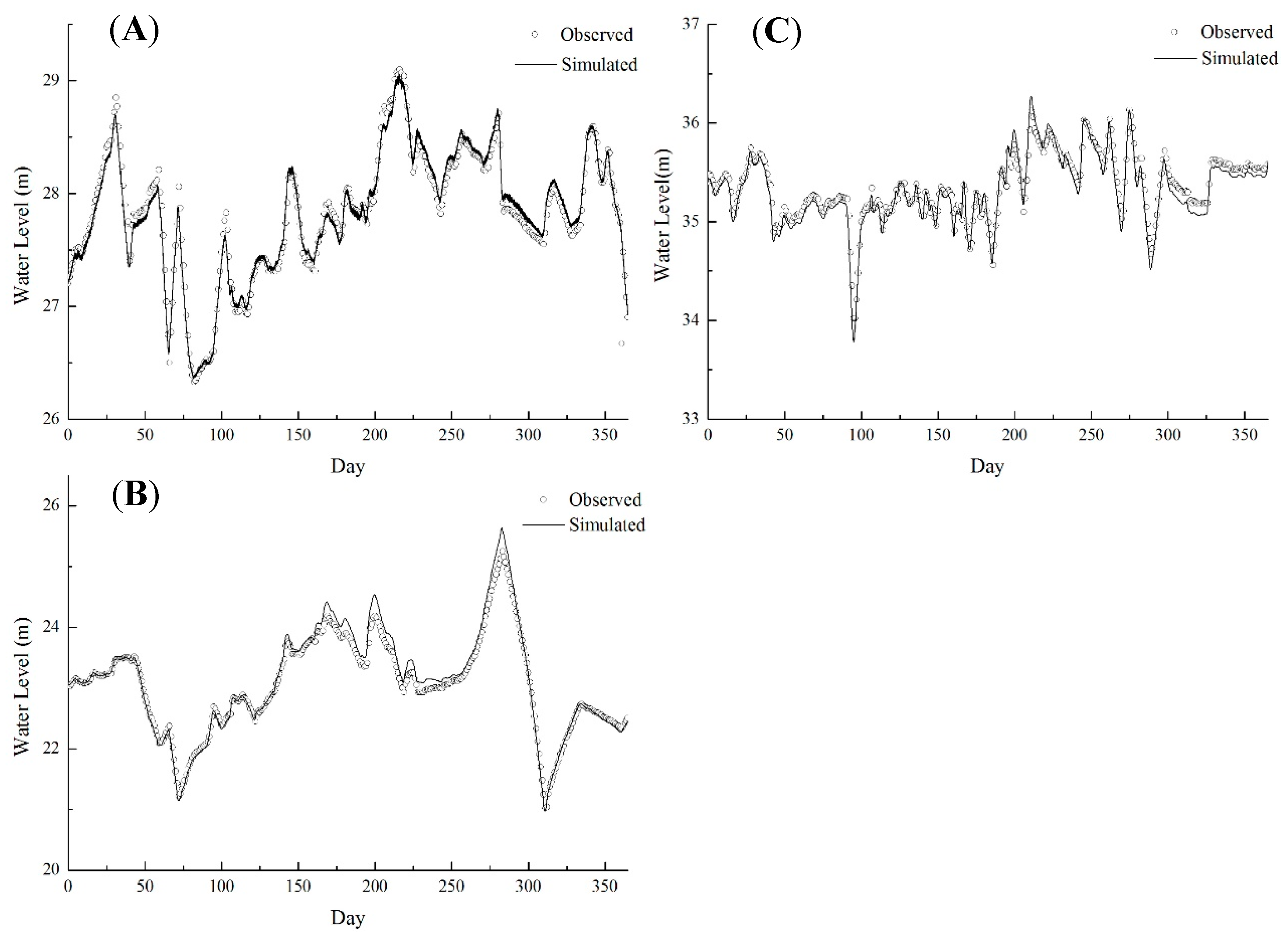
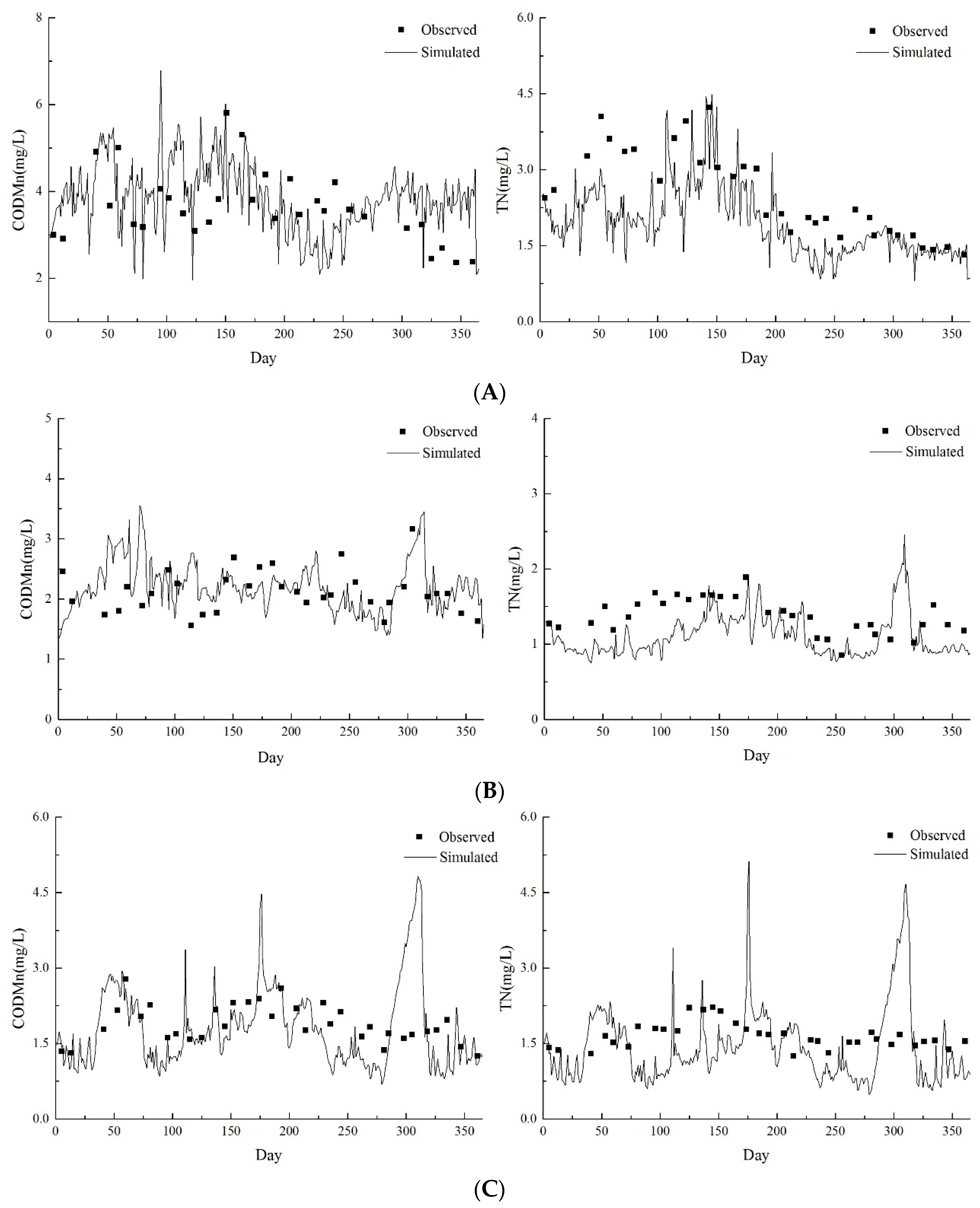
As one of the most important water sources of urban water supply in China, the reservoir water quality directly affects urban water supply security. Hydrodynamics and water quality models can be used to describe the spatial and temporal distributions of water quality variables and provide technical support for water environment management. In our study, a three-dimensional surface water modeling system (EFDC) was used to establish hydrodynamic and water quality model for the regulated cascade reservoirs. The relationships between water quality and improvement measures were quantified and the main pollution sources were identified for individual reservoirs. Results showed the following:

(1)

The hydrodynamic and water quality processes in the regulated cascade reservoirs were well simulated by EFDC. The correlation coefficients of water level simulation in the Shiyan, Tiegang and Xili Reservoirs reached 0.97, 0.997, and 0.98, respectively. The mean absolute errors were only 0.09 m, 0.08 m, and 0.08 m, respectively. Models could well reproduce spatiotemporal heterogeneity of water quality concentrations (COD_Mn and TN). Due to the dramatic decrease in water level in the last three months, the simulated water quality concentrations of the Xili Reservoir were overestimated, and the performance was not as good as that of the Shiyan and Tiegang Reservoirs.

(2)

An increase of transferred water volume, or pollution load reductions of local runoff and transferred water, would improve the water quality conditions in the cascade reservoirs. The most effective method for water quality improvement was to reduce local runoff load for TN and transferred water load for COD_Mn in the Shiyan Reservoir, reduce transferred water load in the Tiegang Reservoir, and increase transferred water volume, especially in the flood season, in the Xili Reservoir.

(3)

To improve the water quality of cascade reservoirs in Shenzhen, the control of diffuse rainfall-runoff pollution should be a priority and can be achieved by establishing a sewage discharge permission system, constructing ecological river wetlands, and other physical and biological measures. In addition, sedimentation should be cleaned up regularly to reduce internal pollution, particularly for the Shiyan and Xili Reservoirs. For the cost–benefit analysis, the combination of water transfer and local river treatment is a probable economic strategy for water quality improvement.

Due to the severe disturbance of the Water Diversion Project, the water quality simulation was very complicated. Although the TN simulation performance was slightly weak, COD_Mn concentrations were simulated satisfactorily, particular for the water level. All the simulation performances were superior to those performed in the Shanmei Reservoir and Danjiangkou Reservoir of China [51,52]. The simulation performance will be further improved and validated if more observations from different years are collected. Other water quality variables, such as total phosphorus, dissolved oxygen, water temperature, and chlorophyll, should be also simulated with consideration of interaction mechanisms among different variables. Moreover, the ensemble Kalman filter may be a good way to assimilate water quality variables and make significant simulation improvements [35].

References

1. Li, S.T. Urban Water Pollution Issues. China Youth. Available online: http://news.xinhuanet.com/environment/2006-09/13/content_5084123.htm (accessed on 13 September 2006).
2. MWR (Ministry of Water Resources, P.R. China). The 11th Five-Year Plan of National Water Resources Development. In Gazette of the Ministry of Water Resources of the P.R. China; MWR: Beijing, China, 2007; pp. 34–48. [Google Scholar]
3. Zhou, Y.; Khu, S.T.; Xi, B.; Su, J.; Hao, F.; Wu, J.; Huo, S. Status and challenges of water pollution problems in China: Learning from the European experience. Environ. Earth Sci. 2014, 72, 1243–1254. [Google Scholar] [CrossRef]
4. MEP (Ministry of Environmental Protection). Report on the State of Environment in China 2014. Available online: http://jcs.mep.gov.cn/hjzl/zkgb/2014zkgb/ (accessed on 3 May 2016).
5. Liu, J.; Diamond, J. China’s environment in a globalizing world. Nature 2005, 435, 1179–1186. [Google Scholar] [CrossRef] [PubMed]
6. Jiang, Y. China’s water scarcity. J. Environ. Manag. 2009, 90, 3185–3196. [Google Scholar] [CrossRef] [PubMed]
7. Whitehead, P.G.; Barbour, E.; Futter, M.N.; Sarkar, S.; Rodda, H.; Caesar, J.; Butterfield, D.; Jin, L.; Sinha, R.; Nicholls, R.; et al. Impacts of climate change and socio-economic scenarios on flow and water quality of the Ganges, Brahmaputra and Meghna (GBM) river systems: Low flow and flood statistics. Environ. Sci. Process. Impacts 2015, 17, 1057–1069. [Google Scholar] [CrossRef] [PubMed]
8. Wang, Q.; Yang, Z. Industrial water pollution, water environment treatment, and health risks in China. Environ. Pollut. 2016, 218, 358–365. [Google Scholar] [CrossRef] [PubMed]
9. Wang, Y.H.; Jiang, Y.Z.; Liao, W.H.; Gao, P.; Huang, X.M.; Wang, H. 3-D hydro-environmental simulation of Miyun Reservoir, Beijing. J. Hydro-Environ. Res. 2014, 8, 383–395. [Google Scholar] [CrossRef]
10. Scavia, D.; Kelly, E.L.A.; Hagy, J.D. A simple model for forecasting the effects of nitrogen loads on Chesapeake Bay hypoxia. Estuaries Coasts 2006, 29, 674–684. [Google Scholar] [CrossRef]
11. Zou, R.; Lung, W.S.; Wu, J. Multiple-pattern parameter identification and uncertainty analysis approach for water quality modeling. Ecol. Model. 2009, 220, 621–629. [Google Scholar] [CrossRef]
12. Wang, S.; Qian, X.; Han, B.P.; Luo, L.C.; Hamilton, D.P. Effects of local climate and hydrological conditions on the thermal regime of a reservoir at Tropic of Cancer, in southern China. Water Res. 2012, 46, 2591–2604. [Google Scholar] [CrossRef] [PubMed]
13. Lindim, C.; Becker, A.; Grüneberg, B.; Fischer, H. Modelling the effects of nutrient loads reduction and testing the N and P control paradigm in a German shallow lake. Ecol. Eng. 2015, 82, 415–427. [Google Scholar] [CrossRef]
14. Norton, D.J.; Wickham, J.D.; Wade, T.G.; Kunert, K.; Thomas, J.V.; Zeph, P. A method for comparative analysis of recovery potential in impaired waters restoration planning. Environ. Manag. 2009, 44, 356–368. [Google Scholar] [CrossRef] [PubMed]
15. Hu, L.; Hu, W.; Zhai, S.; Wu, H. Effects on water quality following water transfer in Lake Taihu, China. Ecol. Eng. 2010, 36, 471–481. [Google Scholar] [CrossRef]
16. He, G.J.; Fang, H.W.; Bai, S.; Liu, X.B.; Chen, M.H.; Bai, J. Application of a three-dimensional eutrophication model for the Beijing Guanting Reservoir, China. Ecol. Model. 2011, 222, 1491–1501. [Google Scholar] [CrossRef]
17. Zhao, L.; Li, Y.; Zou, R.; He, B.; Zhu, X.; Liu, Y.; Wang, J.; Zhu, Y. A three-dimensional water quality modeling approach for exploring the eutrophication responses to load reduction scenarios in Lake Yilong (China). Environ. Pollut. 2013, 177, 13–21. [Google Scholar] [CrossRef] [PubMed]
18. Liang, S.; Jia, H.; Yang, C.; Melching, C.; Yuan, Y. A pollutant load hierarchical allocation method integrated in an environmental capacity management system for Zhushan Bay, Taihu Lake. Sci. Total Environ. 2015, 533, 223–237. [Google Scholar] [CrossRef] [PubMed]
19. Zeng, Q.H.; Qin, L.; Li, X. The potential impact of an inter-basin water transfer project on nutrients (nitrogen and phosphorous) and chlorophyll a of the receiving water system. Sci. Total Environ. 2015, 2536, 675–686. [Google Scholar] [CrossRef] [PubMed]
20. Javaheri, A.; Babbar-Sebens, M.; Miller, R.N. From skin to bulk: An adjustment technique for assimilation of satellite-derived temperature observations in numerical models of small inland water bodies. Adv. Water Resour. 2016, 92, 284–298. [Google Scholar] [CrossRef]
21. Ji, Z.G.; Hu, G.; Shen, J.; Wan, Y. Three-dimensional modeling of hydrodynamic processes in the St. Lucie Estuary. Estuar. Coast. Shelf Sci. 2007, 73, 188–200. [Google Scholar] [CrossRef]
22. Çalışkan, A.; Şebnem, E. Effects of Selective Withdrawal on Hydrodynamics of a Stratified Reservoir. Water Resour. Manag. 2009, 23, 1257–1273. [Google Scholar] [CrossRef]
23. Liu, X.; Huang, W. Modeling sediment resuspension and transport induced by storm wind in Apalachicola Bay, USA. Environ. Model. Softw. 2009, 24, 1302–1313. [Google Scholar] [CrossRef]
24. Jeong, S.; Yeon, K.; Hur, Y.; Oh, K. Salinity intrusion characteristics analysis using EFDC model in the downstream of Geum River. J. Environ. Sci. 2010, 22, 934–939. [Google Scholar] [CrossRef]
25. Wang, Y.; Wang, H.; Bi, N.; Yang, Z. Numerical modeling of hyperpycnal flows in an idealized river mouth. Estuar. Coast. Shelf Sci. 2011, 93, 228–238. [Google Scholar] [CrossRef]
26. Wu, G.; Xu, Z. Prediction of algal blooming using EFDC model: Case study in the Daoxiang Lake. Ecol. Model. 2011, 222, 1245–1252. [Google Scholar] [CrossRef]
27. Zhou, J.; Falconer, R.A.; Lin, B. Refinements to the EFDC model for predicting the hydro-environmental impacts of a barrage across the Severn Estuary. Renew. Energy 2014, 62, 490–505. [Google Scholar] [CrossRef]
28. Arifin, R.R.; James, S.C.; Pitts, D.A.; Hamlet, A.F.; Sharma, A.; Fernando, H.J. Simulating the thermal behavior in Lake Ontario using EFDC. J. Great Lakes Res. 2016, 42, 511–523. [Google Scholar] [CrossRef]
29. State Council of the People’s Republic of China. Water Pollution Prevention Action Plan. Available online: http://www.gov.cn/zhengce/content/2015-04/16/content_9613.htm (accessed on 7 June 2017). (In Chinese)
30. National Environmental Protection Bureau (NEPB). Standard Methods for the Examination of Water and Wastewater (Version 4); China Environmental Science Publish Press: Beijing, China, 2002. (In Chinese)
31. Hamrick, J.M.; Mills, W.B. Analysis of water temperatures in Conowingo Pond as influenced by the Peach Bottom atomic power plant thermal discharge. J. Environ. Sci. Policy 2000, 3, 197–209. [Google Scholar] [CrossRef]
32. Bai, S.; Lung, W.S. Modeling sediment impact on the transport of fecal bacteria. Water Res. 2005, 39, 5232–5240. [Google Scholar] [CrossRef] [PubMed]
33. Liu, Z.; Hashim, N.B.; Kingery, W.L. Fecal coliform modeling under two flow scenarios in St. Louis Bay of Mississippi. J. Environ. Sci. Health 2010, 45, 282–291. [Google Scholar] [CrossRef] [PubMed]
34. Gong, W.; Wang, Y.; Jia, J. The effect of interacting downstream branches on saltwater intrusion in the Modaomen Estuary, China. J. Asian Earth Sci. 2012, 45, 223–238. [Google Scholar] [CrossRef]
35. Kim, K.; Park, M.; Min, J.H.; Ryu, I.; Kang, M.R.; Lan, J.P. Simulation of algal bloom dynamics in a river with the ensemble Kalman filter. J. Hydrol. 2014, 519, 2810–2821. [Google Scholar] [CrossRef]
36. Blumberg, A.F.; Mellor, G.L. A description of a three dimensional coastal ocean circulation model. In Three-Dimensional Coastal Ocean Models, Coastal and Estuarine Science; Heaps, N.S., Ed.; American Geophysical Union: Washington, DC, USA, 1987; pp. 1–19. [Google Scholar]
37. Hamrick, J.M. A three-dimensional Environmental Fluid Dynamics Computer Code: Theoretical and computational aspects. In Special Report in Applied Marine Science and Ocean Engineering; No. 317; Virginia Institute of Marine Science (VIMS): Gloucester Point, VA, USA, 1992. [Google Scholar]
38. Lin, J.; Li, J. Nutrient response modeling in falls of the Neuse Reservoir. Environ. Manag. 2011, 47, 398–409. [Google Scholar] [CrossRef] [PubMed]
39. Cerco, C.F.; Cole, T.M. Three-dimensional eutrophication model of Chesapeake Bay. J. Environ. Eng. 1993, 119, 1006–1025. [Google Scholar] [CrossRef]
40. Tetra Tech, Inc. The Environmental Fluid Dynamics Code Theory and Computation Volume 3: Water Quality Module; Tetra Tech, Inc.: Fairfax, VA, USA, 2007. [Google Scholar]
41. Naoum, S.; Tsanis, I.K.; Fullarton, M. A GIS pre-processor for pollutant transport modelling. Environ. Model. Softw. 2005, 20, 55–68. [Google Scholar] [CrossRef]
42. Tang, T.; Yang, S.; Yin, K.; Zhou, R. Simulation of eutrophication in Shenzhen Reservoir based on EFDC model. J. Lake Sci. 2014, 26, 393–400. (In Chinese) [Google Scholar]
43. Moriasi, D.N.; Arnold, J.G.; Van Liew, M.W.; Binger, R.L.; Harmel, R.D.; Veith, T. Model evaluation guidelines for systematic quantification of accuracy in watershed simulations. Trans. ASABE 2007, 50, 885–900. [Google Scholar] [CrossRef]
44. Wei, J.; Zeng, H.; Qing, H.; Ma, Z.B. Effects of spatial variability of land use on water quality within Shiyan Reservoir watershed in Shenzhen City. China Environ. Sci. 2008, 28, 938–943. (In Chinese) [Google Scholar]
45. Wang, Y.; Hao, X.; Fu, J.; Sheng, G. Water quality change in reservoirs of Shenzhen, China: Detection using LANDSAT/TM data. Sci. Total Environ. 2004, 328, 195–206. [Google Scholar] [CrossRef] [PubMed]
46. House, W.A.; Denison, F.H.; Smith, J.T.; Armitage, P.D. An investigation of the effects of water velocity on inorganic phosphorus influx to a sediment. Environ. Pollut. 1995, 89, 263–271. [Google Scholar] [CrossRef]
47. Qin, B.; Zhu, G.; Zhang, L.; Luo, L.; Gao, G.; Binhe, G.U. Estimation of internal nutrient release in large shallow Lake Taihu, China. Sci. China Ser. D Earth Sci. 2006, 49, 38–50. [Google Scholar] [CrossRef]
48. Hu, K.M.; Wang, S.; Pang, Y. Suspension-sedimentation of sediment and release amount of internal load in Lake Taihu. J. Lake Sci. 2014, 26, 191–199. (In Chinese) [Google Scholar]
49. Heyuan Environmental Protection Bureau. Available online: http://www.hydp-reform.gov.cn/a/zhengwugongkai/tongzhigonggao/2016/0802/843.html (accessed on 29 August 2017). (In Chinese)
50. Water Resources Bureau of Shenzhen Municipality. Available online: http://www.szwrb.gov.cn/bsfw_77954/bmxx/pshjs_80980/wsclf/ (accessed on 29 August 2017). (In Chinese)
51. Chen, L.B.; Yang, Z.F.; Liu, H.F. Assessing the eutrophication risk of the Danjiangkou Reservoir based on the EFDC model. Ecol. Eng. 2016, 96, 117–127. [Google Scholar] [CrossRef]
52. Liu, M.B.; Chen, X.W.; Yao, H.X.; Chen, Y. A coupled modeling approach to evaluate nitrogen retention within the Shanmei Reservoir watershed, China. Estuar. Coast. Shelf Sci. 2015, 166, 189–198. [Google Scholar] [CrossRef]
Figure 1. Locations of the cascade reservoirs and their surrounding land uses. TX: Connected Project; ST: a water project taking water from Tiegang Reservoir to the Shiyan Reservoir; T1: Jiuwei River; T2: Huangmabu River; T3: Tangtou River; X1: Baimang River; X2: Dongshen Water Supply Project; X3: Makan River.
Water 09 00825 g001
Figure 2. Computational grids for hydrodynamic and water quality simulations in the cascade reservoirs.
Water 09 00825 g002
Figure 3. Simulated and observed water level in the Shiyan (A), Tiegang (B) and Xili (C) Reservoirs.
Water 09 00825 g003
Figure 4. Simulated and observed concentrations of CODMn and TN in the Shiyan (A), Tiegang (B), and Xili (C) Reservoirs.
Water 09 00825 g004
Figure 5. Simulated spatial distributions of CODMn and TN concentrations in the Shiyan (A), Tiegang (B) and Xili (C) Reservoirs. Note: Six grades were used according to the Chinese Environmental Quality Standards for Surface Water (GB3838-2002).
Water 09 00825 g005
Figure 6. Improvement of water quality under increasing proportions of transfer water during the non-flood season (A) and flood season (B) in the Xili Reservoir.
Water 09 00825 g006
Figure 7. Water quality improvement on reducing different proportions of transferred water pollution load in the Tiegang Reservoir: CODMn (A); TN (B).
Water 09 00825 g007