On the Direct Calculation of Snow Water Balances Using Snow Cover Information
by
 and
and
Alberto Pistocchi
1,*, 
Stefano Bagli
2,
Mattia Callegari
3,
Claudia Notarnicola
3 and
Paolo Mazzoli
2 1
European Commission DG JRC, Directorate D Sustainable Resources. Via E.Fermi, 2749–21027 Ispra (VA), Italy
2
GECOsistema srl, viale G.Carducci, 15, I-47023 Cesena (FC). R&D Unit Suedtirol. Via Maso della Pieve/Pfarrhofstr., 60A–39100 Bolzano/Bozen, Italy
3
EURAC Research, Institute for Applied Remote Sensing; viale Druso, 1–39100 Bolzano, Italy
*
Author to whom correspondence should be addressed.
Water 2017, 9(11), 848; https://doi.org/10.3390/w9110848
Submission received: 11 April 2017
/
Revised: 24 October 2017
/
Accepted: 24 October 2017
/
Published: 2 November 2017
Abstract
:We present a novel method for the direct determination of the snowmelt coefficient of widely used degree-day models, using only cumulated temperature and precipitation over the days of snow cover. We develop a proof of concept using (1) local measurements of precipitation, temperature and snow water equivalent (SWE) at a set of well-monitored sites in the US, and (2) available time series of snow cover from satellite and gridded daily precipitation and daily average temperature for the study region of South Tyrol, in the Italian Alps. We demonstrate how the method can reproduce the snow water balance to an acceptable extent, critically depending on the accuracy of input precipitation and temperature, highlighting the importance of a reliable representation of weather forcing if the estimate has to be robust and representative. Although not always accurate at a point, our approach yields a SWE reasonably consistent with observations, and snowmelt flows compatible with measured streamflow. At the same time, the model allows an interpretation of discrepancies between observations and simulations to detect inconsistencies between snow cover and weather forcing. This method is in principle applicable for large-scale hydrological assessments thanks to the increasing global coverage of snow cover, precipitation and temperature data. As the only other type of observation available to calibrate models is often streamflow, the direct calibration of the snow component of a model using snow cover and weather forcing reduces the number of model processes and parameters to be calibrated with streamflow, and is expected to increase model robustness.
1. Introduction
Snow water equivalent (SWE) and snowmelt fluxes are variables of great importance in the assessment of water resources in mountain regions. Although SWE earth observation products exist [1,2], the evaluation of quantities of water stored as snowpack is still problematic due to the large variability of snow density and depth following morphological and climatic conditions on terrain. Space-borne remote sensing SWE estimation is mainly achieved with passive microwave sensors, but it can only reach a coarse resolution [3,4], limiting its use for water resources assessment at the catchment scale.
Other than from remote sensing, SWE may be evaluated through statistical regionalization of SWE [5,6,7] capitalizing on the availability of several measurements of snow in space, possibly including non-conventional variables (e.g., the distribution of climatologically averaged SWEs using tree ring series [8]). Observations, though, remain sparse and even totally absent in certain regions, which calls for other ways to regionalize SWE, particularly through spatially distributed hydrological models. These may have various levels of complexity, from the simple degree-day method (DDM: [9,10,11,12]), to comprehensive physically based models of the snowpack energy balance (e.g., [13,14]).
Snow-covered area (SCA) information, mainly from remote sensing products, offers a proxy for the hydrological state of a snow-dominated watershed (see, e.g., [15,16]). As such, it is often used to improve hydrological models either as an additional criterion in multi-objective model parameter calibration (e.g., [17,18,19]) or for assimilation in land surface models (e.g., [20,21,22,23]). SCA is also used as a direct input to DDM-based lumped models to predict snowmelt runoff (e.g., [24]), when calibrating model parameters using streamflow or other data. Molotch and Margulis, [25] (further debated in [26,27]) use SCA information to back-calculate SWE on the basis of a simple snowmelt model with assigned parameters. The potential of snow cover data to directly calculate snow water balances, though, has not been fully exploited until now. He et al. [28] actually use snow cover and depth information to directly estimate snowmelt factors for a DDM-based model, showing improvements in hydrological model performances compared with the case when snowmelt factors are calibrated with the streamflow observations alone. However, snow depth data as used in their approach may not always be available, and a less data-demanding method is desirable.
In this contribution, we propose a novel, alternative approach for the direct and spatially distributed calibration of the DDM, making use of snow cover information from remote sensing in combination with daily precipitation (P) and mean air temperature (T) data alone. We show that the model provides accurate results when the input data are accurate, and we test its limitations when applied to cases where input data are available with lower levels of accuracy. Based on our findings, we finally advocate that a simple estimation of SWE over large regions is possible on the basis of snow cover, P and T alone, and may help improving hydrological models used for water resources assessment at the regional to global scale.
2. Materials and Methods
2.1. The Degree-Day Method
The degree-day method (DDM) is an empirical model assuming snowmelt proportional to the temperature above a threshold accumulated in time (“degree-days”), the proportionality constant being called a “snowmelt coefficient” or “degree-day factor”. Although physically based models are, in principle, more accurate and do not necessarily demand more data [29], hydrological modeling practice has often found relatively little advantage in their use compared to simple models [30,31,32,33]. Also because of this, DDM is still widely adopted in hydrology, especially at regional scales and for basins in remote regions (e.g., [34,35,36,37,38,39,40,41,42,43,44]), and when air temperature-dependent turbulent heat transfer and longwave radiation account for most of the snowmelt (e.g., [12]).
Some authors suggest including a linear dependence on a radiation proxy as well as on accumulated air temperature [43,45,46]. In the Precipitation, Runoff, Evapotranspiration Hydrotope (PREVAH) model [47], the snowmelt factor is allowed to depend on wind speed, saturation vapor pressure and rain. While this formulation is in principle quite general, information on wind speed and air vapor pressure is not commonly available, particularly in mountain regions.
Corrections to the basic DDM have been proposed to allow relaxing the assumption of strictly linear relations between accumulated temperature and snowmelt. Certain formulations correct the snowmelt coefficient for the melting acceleration effect of rain on snow (e.g., in the LisFlood model [48]). Another common correction to the snowmelt factor addresses the predictable seasonal variability of energy input to the snowpack (e.g., by introducing a sinusoidal function as a multiplier, as in the Soil-Water Assessment Tool (SWAT) model [49], as well as LisFlood [48]. As for the spatial variability of snowmelt, Cazorzi and Della Fontana [50], invoking a hydrologic similarity concept for sites with similar solar energy supply, assume the snowmelt coefficient to be proportional to a topography-driven energy index, related to potential daily average solar radiation. This accommodates for a high variability of snowmelt depending on elevation, slope orientation and shading, at the same time keeping computations very simple.
The DDM does not account for snow transport by wind, nor for snow sublimation. The former is important at scales of hundreds of meters (e.g., [51]), while wind-transported snow is assumed to be completely sublimated at distances in the order of 3000 m (e.g., [52]), suggesting wind transport may be neglected when working at regional to river basin scales. Snow sublimation from wind blow has been quantified in ranges from less than 10% of the snow balance [53,54] to around 20% [55,56] and sometimes even around 30% [57]. These figures suggest a plausible upper range of the error on the estimation of snowmelt using the DDM due to neglecting this process.
In this work, we assume the parameterization of the snowmelt coefficient used in LisFlood [48], a spatially distributed hydrological model extensively used for water resources assessment at the European scale: on a given day, snowmelt is proportional to temperature above a snowmelt temperature threshold (assumed here to be 0 °C), through the coefficient:
where C0 is a constant (mm/°C day), R is rain on snow (mm/day), di is the day of the year (1 = 1 January) and α and β are appropriate coefficients. We take default values β = 0.01 and α = 0.25 consistently with [48]. While a systematic sensitivity analysis of the model to these parameters is beyond the scope of this paper, some casual trials varying these default values indicated limited impact on the overall results. This formulation accounts for the dependence of snowmelt on the seasonal pattern of radiation and on the energy conveyed by rainfall on snow, and is chosen for its simplicity while maintaining a certain flexibility. Rain on snow is estimated as precipitation multiplied by 1 − f(Ti), where is the fraction of precipitation that is snowfall form during the day with average temperature Ti. The latter is predicted here as f(Ti) = max(0,min(1,1 − Ti/Tprec)), Tprec = 1 °C being a threshold temperature above which all precipitation is considered as liquid (see [58,59]).
2.2. Direct Estimation of the DDM Snowmelt Factor
With reference to a period of continuous snow cover, we may write the following balance of snowfall and snowmelt:
where n is the number of days composing the continuous snow cover period, and Pi and Ti are daily precipitation and temperature. From Equation (2) we can compute C0 explicitly from Y, X1, X2 and X3, obtained directly from series of precipitation and temperature over a period of continuous snow cover for a given site, as:
where
C0 = Y/(0.01 × X1 + X2 + 0.25 × X3)
Periods of continuous snow cover may be detected, in principle, from field or satellite snow observations. Field observations, though, are only available at measurement sites, while satellite images suffer from errors due to cloud cover and other artifacts (see, e.g., [60]) that create spurious interruptions of snow cover. Cumulates Y, X1, X2 and X3 computed on the arbitrary snow cover periods resulting from these interruptions cannot correctly reflect the balance of snowfall and snowmelt. In order to overcome this problem, we make the additional working assumption that Equation (3) holds also when computing Y, X1, X2 and X3 as the cumulates of all values during snow cover days over an extended period.
2.3. Testing the Approach at Sites with Accurate Data
The approach has been tested to reproduce snow water equivalent measured at seven sites (see Table 1) of the Snow Telemetry (SNOTEL) network [61] operated by the US Natural Resources Conservation Service (NRCS), located in the Upper Rio Grande basin in Colorado, where a DDM was already successfully applied [62].
The SNOTEL network provides direct, co-located and simultaneous measurements of SWE and weather forcing, and represents near-ideal situations for the application of the method. In order to compute the cumulates Y, X1, X2, X3 to estimate C0 in Equation (3), we considered at each station all days with SWE > 0 as snow-covered.
2.4. Testing the Approach Using Regional Information
In order to appreciate the impact of using regionalized information on the performance of the method, we consider as a test region the upper Adige catchment, covering most of South Tyrol in the Italian Alps (Figure 1). The area is approximately 7400 km2, of which about 80% lays between 1000 and 2900 m a.s.l., with peaks up to about 3800 m a.s.l.
The region has annual average temperatures between more than 12 °C in the valley bottoms, and less than −4 °C in the higher ranges. Annual precipitation ranges between less than 600 mm (in the deeper valleys on the west side of the region) and more than 2000 mm (in the northeastern end), with a general trend of yearly precipitation increasing with elevation and moving roughly southwest to northeast. Kottek et al. [63] place the region in the Koeppen-Geiger climate classes Dfb, Dfc and ET. Snow cover usually starts between early November and mid-December, depending on the altitude, and ends from end of March to end of May at the higher elevations, with spots showing almost permanent snow cover and glaciers. The duration of snow cover is clearly correlated with elevation and ranges from a few days up to more than 200 days yearly. Low-lying valley bottoms, below 1000 m with the southernmost part of the area close to 200 m a.s.l., show much shorter and intermittent snow cover periods.
The regionalized information available in South Tyrol includes a 250 m resolution daily snow cover time series from 1 November to 31 May based on the well-known Moderate Resolution Imaging Spectroradiometer (MODIS) for winters 2002–2003 till 2009–2010, and a time series of daily gridded precipitation and temperature obtained from the interpolation of existing weather stations.
Snow cover maps are produced on a regular basis by EURAC Research, Bolzano [64] using the algorithms of [65,66], developed in order to keep the resolution as high as possible in order to improve snow detection, especially in mountainous areas characterized by complex terrain.
Daily gridded values of average temperature and precipitation were derived, in the context of early developments of a regional soil water balance model [67] from temperature and precipitation measurements at ground stations operated by the province of Bolzano’s Hydrographic Office (see [16] for details) using regression kriging with external drift (given by elevation) for temperature, and ordinary kriging for precipitation. The choice of ordinary kriging was due to the unclear patterns of correlation between precipitation and elevation emerging from the analysis of the available data. The interpolation was performed with a resolution of 1 km, using the raw data available after filtering out unrealistically high or low values in the daily time series at stations.
All over the region, 16 snow depth measurement sites were made available by the Hydrographic Office of the province of Bolzano (indicated in Figure 1; additional data in Table 2 and Table 3), where temperature and precipitation were not systematically measured. Also, systematic snow density measurements are not available. However, Pistocchi [68] shows that snow density in South Tyrol can be described fairly well with the simple equation ρ = 0.2 + 0.001 DOY (with ρ = snow density in t/m3, DOY = day number from beginning of snow season).
For the testing of snowmelt, we identified eight headwater catchments (Figure 1) for which discharge measurements are available. The characteristics of catchments and discharge gauging stations are provided in Table 4.
2.4.1. Testing Modelled SWE at Snow Depth Measurement Stations
We extracted a time series of interpolated temperature and precipitation and a time series of snow cover presence/absence (0/1) for pixels corresponding to the 16 snow measurement stations. Snow cover maps from MODIS contain inevitably several pixels with no data due to clouds or other artifacts. Moreover, misclassification of snow pixels is far from a rare event. Cloud clearing methods based on the temporal combination of successive observation days have successfully been applied in many studies (e.g., [2,69,70]). These methods are known to affect the overall accuracy of the snow cover series depending on the number of days that are employed in the cloud clearing process. For instance, the temporal combination of two successive days is successful in around 90% of cases, as shown by [71]. In the present exercise, given the relatively high number of cloudy days at the sites of interest, pixels classified as “clouds” were assigned to either snow or non-snow based on the predominant condition in a moving time window set from five days before to five days after each day in order to avoid discarding too many days, likely with snow cover, in the calculation of the cumulates.
From the snow cover, precipitation and temperature time series, we computed the cumulates Y, X1, X2 and X3, considering all days in the winters (November to May) of the period 2002–2010, in which a pixel is classified as “snow-covered”. Consequently, it is possible to compute a snowmelt coefficient constant C0 from Equation (3), hence snowmelt (M) and snow water equivalent (SWE) as:
where t denotes a generic day in the year, M(t), P(t) and T(t) are the corresponding daily values of snowmelt, precipitation and temperature, respectively, S(t) is a binary variable equal to 0 if snow cover is absent, and to 1 if it is present, and C is computed from Equation (1). SWE can be computed on a daily basis for each site where snow cover, precipitation and temperature are known, and can be compared in particular with SWE from measured snow depth and estimated density at the 16 observation sites. It should be noted that, in Equation (4), all quantities are referred to a unit surface area and can be therefore expressed in mm, mm/day or other consistent units.
It should be noted that, by computing C0 as the ratio of cumulative snowfall (P) to a combination of cumulative positive degree-days (T) and rainfall times positive temperature (P × T) over all snow-covered days of the snow cover time series, we implicitly assume this ratio to be representative of the balance between snowfall and snowmelt. We may plot the ratio of cumulates P, T and P × T over snow-covered days for all stations from the start of the period to a generic end date (as shown in the Supporting Information, Figure S1). In principle, this ratio may converge to a constant value, but it can also show a trend. When it converges, we may assume that a representative constant snowmelt coefficient is an appropriate assumption. A trend, on the contrary, indicates that a single constant representative coefficient cannot be identified based on the available information. Across the 16 sites examined in the Supporting Information, a trend appears only in two cases, suggesting that the problem may be limited in practical applications.
2.4.2. Testing Modelled Melt Flows at Headwater Discharge Measurement Stations
We also extracted snow cover, precipitation and temperature information for the cells of a 1 km resolution grid corresponding to selected headwater catchments (Table 4) and repeated for each grid cell the exercise conducted for the snow depth station points. Each grid cell was considered snow-covered if this was the dominant condition among the 16 grid cells of the 250 m resolution MODIS-derived snow cover image. The calculation yields daily snowmelt flows per pixel according to Equation (4), which were summed over each catchment to represent total snowmelt discharge. These flows, only for days of the months of March, April and May when we expect significant contributions from snowmelt, were compared to observed discharges.
3. Results and Discussion
3.1. Snowmelt Coefficients and Snow Water Equivalents at SNOTEL Sites
Table 1 lists, for the seven sites, the values estimated for C0 along with average daily snowmelt coefficients calibrated by DeWalle et al. [62].
The coefficients found with our approach are lower, but correlated with those of DeWalle et al. [62]. The differences may be attributed to the different assumptions in ours and their model, and the different averaging periods. With the values of C0 in Table 1, the model of Equation (4) reproduces to an acceptable level of accuracy the time series of measured SWE at all stations (results shown as Supporting Information). This indicates the validity of the approach when applied at sites where accurate information is available.
3.2. Snowmelt Coefficients and Snow Water Equivalents at Snow Depth Measurement Stations
Estimated snowmelt coefficients for the 16 sites of this study are provided in Table 3. SWE simulated from Equation (4) using these snowmelt coefficients can be compared with SWE derived from measurements of depth and estimates of snow density (hereinafter considered as “observed” SWE), as in the example of Figure 2 (graphs for the remaining stations are provided as Supporting Information Figure S2). While in all stations a reasonable correspondence of observed and simulated SWE can be found for at least some winter seasons, the performance of the model shows considerable variability, and in many cases it remains rather weak, as indicated by the summary of model performance indicators provided in Table 3. The model yields systematic underestimation of SWE at most stations, a quite common outcome in snow modelling studies (e.g., [72,73]). Artan et al. [73] identify the main source of underestimation in the negative bias of gridded precipitation data compared with measurements at SWE gauging sites. This is reflected in a systematic error (MSEs% [74]), usually dominating over the unsystematic error (MSEu%; ibid.). The root mean squared error (RMSE) is usually twice (or more) the uncertainty of observed SWE (whose upper bound is around 35% due to snow density uncertainty [68]). The Nash-Sutcliffe efficiency (NSE) of the model is usually rather poor, which is somehow expected as this indicator reflects the level of agreement on the higher values (e.g., [75]), but negative NSE values indicate the observed mean is a better predictor of SWE than the model. The index of agreement d [20] and the R2 are more encouraging, although not in all cases (d should be considered acceptable above at least 0.7, see, e.g., [75]). In some cases, the extremely low proportion of variance explained owes to one specific winter season where observations are completely unrelated to simulations. For instance, if we consider the station of Ciampinoi (code X112Y63), removing winter 2006–2007 increases R2 from about 4% to more than 40%. The large overestimation of SWE by the model during this season is likely related to an error in precipitation, that results four to six times higher than during the other winters. In fact, during this period the nearest precipitation station systematically records anomalously high precipitation values that could not be automatically filtered out from the time series prior to interpolation.
Although the model performance indicators (Table 3) have no significant correlation with the snowmelt coefficients, NSE at sites with low values of snowmelt coefficients is generally negative and the index of agreement d is generally relatively low, suggesting that these situations tend to be modelled less accurately. The values of the snowmelt coefficients are also about a half of typical literature values [11,28,46]: out of 16 sites, six yield snowmelt coefficients below 1 mm/°C day, and only three above 2 mm/°C day. The snowmelt coefficients are negatively and significantly correlated to the cumulative temperature (r = −0.73, p = 1.2E − 03). In turn, T shows a positive correlation with elevation (r = 0.71; p = 1.8E − 03), which is unexpected. Also, we find a positive correlation of T with the number of days where we assumed snow cover under clouds (r = 0.68, p = 3.7E − 03). The correlation with precipitation (P) and precipitation divided by the number of days with snow cover (P/N) is rather low and not significant (r = 0.24, p = 0.37; r = 0.43, p = 0.09, respectively).
Assuming the approach can reproduce SWE under conditions of reliable data (as shown in Section 3.1), the systematic underestimation of SWE and the generally low estimates of C0 may depend on lack of precipitation or excess of temperature over snow-covered days.
Errors in model forcing are known to have an impact on SWE reconstruction [76]. Looking at our case, the measurement sites may not have temperature measurements nearby, and the interpolation may yield local overestimations due to important elevation differences with the nearest measurement stations. We tested the impact of increasing the threshold temperature for melting, and the temperature for 100% liquid precipitation (Tprec) accounting for the temperature adiabatic lapse rate (6.5 °C/1000 m ) at the six stations with snowmelt coefficient below 1 mm/°C day, using for each station an approximate elevation difference representative of the nearest available station. In addition, measurements of snow precipitation are known to suffer from gauge undercatch, and precipitation changes with altitude may be significant. In order to account for the latter effect, the gridded precipitation was corrected for altitudinal effects using a lapse rate in line with the values found by Herrnegger et al. [77]. These temperature and precipitation corrections yield sizeable increases in C0 at all stations, and values in five out of six stations well above 1 and substantially in line with the literature, while the explained variance of measured SWE does not deteriorate or even improves, as shown in the Supporting Information (Table S1). The test indicates that both the underestimation of SWE and the low C0 values obtained in the South Tyrol case may be related to precipitation underestimation and temperature overestimation. A low estimated C0 may be regarded in general as a clue for this type of errors in precipitation and temperature, and prompts to apply appropriate corrections in order to obtain more realistic snowpack balances.
A possible additional cause of discrepancy is in the limitations of satellite-derived SCA in the presence of canopy cover. Correcting satellite data for canopy cover has been shown to increase SCA and SWE, consistently with modelled hydrological balances (see [78]). All stations with C0 < 1 were found to fall in grid cells with significant canopy cover, with the exception of station X75Y48 (Waidmannalm/Hafling). At all 16 stations considered here, however, discrepancies between the number of snow cover days estimated from satellite and the number indicated by positive observed snow depth (Table 2) do not exhibit any significant correlation with the snowmelt coefficients, nor with the model performance, suggesting the impact of the snow cover time series on the estimation of C0 may be limited.
It should be recalled that, when SWE is low, snow cover may not be detected despite some presence of snow. The value of SWE at which snow cover is completely detected is in the order of 10 to 40 mm water, depending on terrain roughness [79], and can be higher in the presence of canopy. In principle, total snowmelt during snow cover must balance not only cumulated snowfall, but an additional amount of water that should logically correspond to the water available on the ground surface when snow cover is no longer fully detected. If we assume this amount to be 15 mm, in the lower range of [79], considering a single snow cover period for each of the eight winter seasons during 2002–2010, the cumulate of snowfall (P in Table 1) must be increased by 15 × 8 = 120 mm, which implies already an increment of the snowmelt coefficient of about 5% (see Supporting Information Table S1). However, in some years there may be more than one continuous period of snow cover, and we should consider a 15 mm increase of P for each new period. In this case, the increment of the snowmelt coefficients would be higher of a factor equal to the average number of continuous snow cover periods in a year (e.g., two or more in some cases).
3.3. Simulated Snowmelt
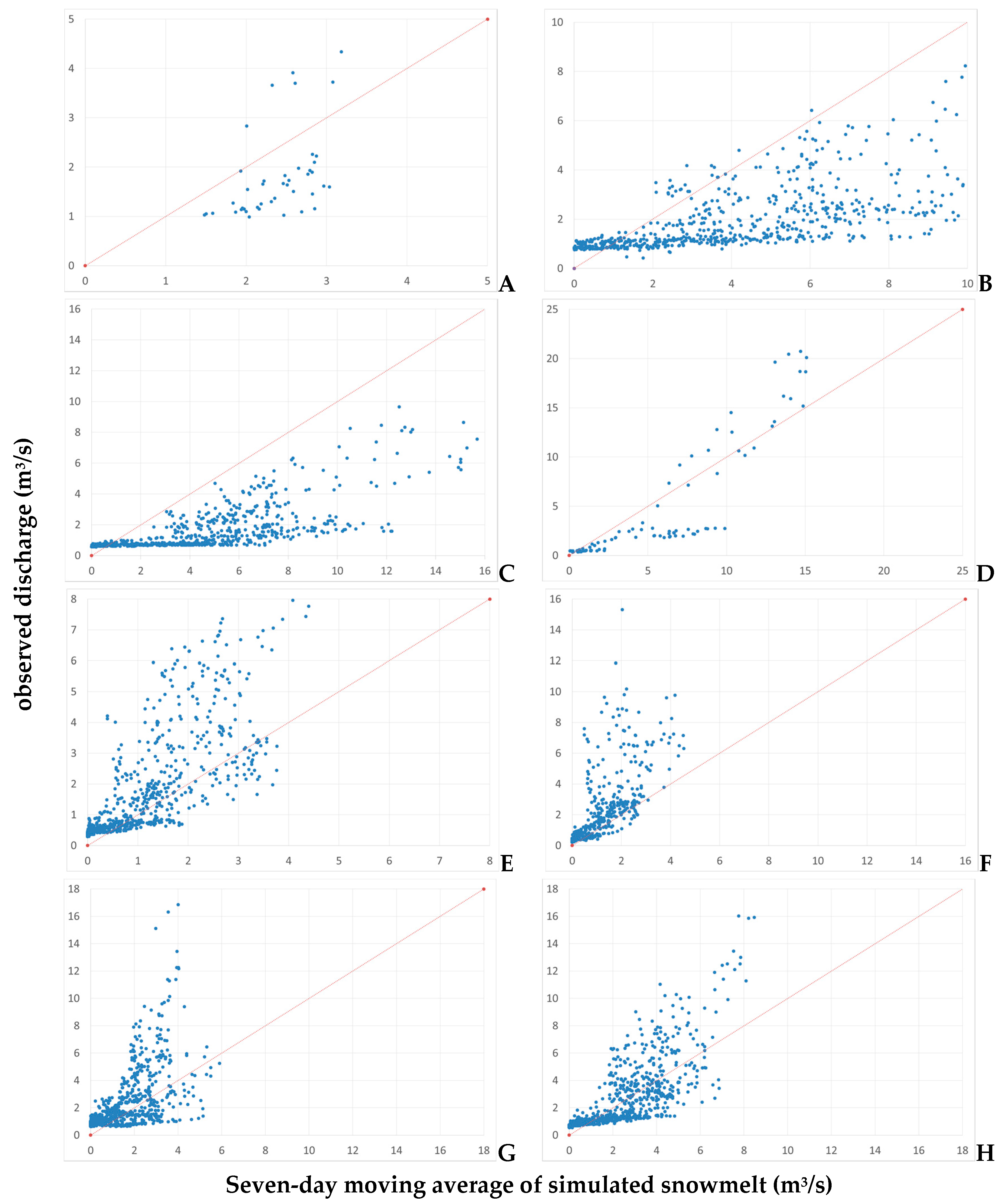
For the eight selected headwater catchments, snowmelt coefficients estimated at the nodes of the 1 km resolution precipitation and temperature grids enabled calculating a time series of SWE and snowmelt on the whole catchment. Simulated snowmelt can be compared with observed discharges, with some caution. First of all, daily values of snowmelt may be very noisy, whereas catchments tend to compensate effects in time by detaining peak flows and releasing them in a smoother way. In mountain catchments of the size considered here, a relatively small snowmelt event may be retained and delayed by all forms of infiltration and ponding. In order to smooth out the variability of snowmelt, and merely for the sake of a semi-quantitative comparison with observed runoff, we conventionally refer to the moving average of snowmelt during seven days. Moreover, the signal of snowmelt in those catchments is expected to be most apparent during the months of March, April and May only, while other processes may play a larger role during the remaining periods. In order to account for these effects, we compare the moving average of snowmelt during seven days with observed discharges for the months of March, April and May of the period 2002–2010 when available. It should be noted that snowmelt occurring on hillslopes should be routed using an appropriate hydrological model in order to describe its detention and transmission losses in the catchment, as other processes, including infiltration, evapotranspiration and subsurface flow, may play a significant role (e.g., [80]). Therefore, the comparison of simulated snowmelt with observed runoff retains only an indicative meaning and, contrary to the case of evaluating a calibrated hydrological model, is not expected to yield a strict correspondence between observed discharges and computed snowmelt. In all cases, however, a significant positive correlation emerges (Table 4), although with apparent dispersion (Figure 3). Station 3415-Vedretta Piana presents a limited number of discharge observations from a catchment influenced by the effect of glaciers and with significant storage in a set of small glacial lakes, which explains the poorer correlation. Still, the range of predicted snowmelt is in good agreement with the range of observed discharges (Figure 3A). In the cases of Station 4575-Rio Casies at Colle (Figure 3B) and Station 4875-Rio Anterselva at Bagni Salomone (Figure 3C), snowmelt overestimates observed discharges. In these catchments, recorded discharges correspond to about 14 L/s per km2, while all other catchments feature between 17 and 26 L/s per km2 (see Table 4). Moreover, the ratio of inflow to outflow is around 7 for the two stations, while for the other six the ratio is between 1 and 3. At low flow values, observed discharges seem to remain relatively constant, while snowmelt varies considerably, and at the lowest values observations are above simulated snowmelt. In the case of Station 5497-Rio Riva at Caminata (Figure 3D), another station with relatively scarce measurements, while an overestimation is still apparent at low flows, the match between snowmelt and runoff is clearly better at higher flows. In the other cases, snowmelt appears less biased in comparison with observations. The dispersion of values at higher flows may be due to other components of runoff in the stream, and particularly rainfall-runoff processes. Despite its indicative and exploratory character, this comparison highlights the compatibility of our simulation with the hydrological processes of these catchments.
4. Conclusions
We have proposed and tested a novel method to derive the snowmelt coefficient of a DDM-based model directly from snow cover and weather data. The method is simple, and yields spatially distributed SWE and snowmelt estimates reasonably consistent with observations. While we do not account for fine-scale spatial variability, the approach may capture watershed-scale variability of melt energy and freezing levels as reflected in the interplay between snow cover and weather forcing, the key element needed in large-scale snow models [81].
An important advantage of independently calibrating the snow module of hydrological models is in reducing the number of hydrological processes (hence model parameters) to be calibrated on the basis of streamflow only. This is expected to improve model robustness, particularly in large-scale water resources assessment, if calibrated models must then be used to estimate variables other than streamflow. It should be stressed that the method for SWE and snowmelt estimation presented here is conditional to a given spatial distribution of precipitation and temperature, as well as snow cover observations. Snowmelt coefficients estimated with our approach may be used to compute snow balance variables from a given temperature and precipitation dataset, but an accurate representation of these variables is critical for the transferability of the estimated coefficients and remains a key requirement along with the representativeness of snow cover information. Hence precipitation and temperature should be carefully checked to remove biases due to elevation gradients, and SWE corresponding to non-detectable snow cover should be accounted for, whenever necessary. Conversely, the method may be used to detect inconsistencies of snow cover with precipitation and temperature data when it yields unrealistic snow melt coefficients. The approach allows in principle a simple operational calculation of SWE and snowmelt, which may be useful for water resources management, especially over large regions. The expanding available capacity to handle satellite information at high resolution globally (see, e.g., [82]) and the development of global precipitation data (e.g., [83]) suggest it could be applied in the future for large scale snow water assessment.
Supplementary Materials
The following are available online at www.mdpi.com/2073-4441/9/11/848/s1. The data used in this research may be obtained upon request to the authors. In a separate document of supporting information, we show an application of the proposed DDM model to the seven measurement stations of Wolf Creek Summit, Culebra#2, Cumbres Trestle, Beartown, Middle Creek, Lily Pond and Trinchera (Colorado, USA), used in the analysis of DeWalle et al. [62], from the well-known Snow Telemetry (SNOTEL) system managed by the US National Resources Conservation Center—National Water and Climate Center. At each station, we use the criterion SWE > 0 to detect presence or absence of snow cover. This corresponds to considering ideal situations where both snow cover and weather forcing are known with the best reasonably achievable accuracy. In all seven cases, C0 results acceptably in line with the literature and, particularly, the findings of DeWalle et al., [62], corroborating the validity of the approach when reliable SCA, precipitation and temperature are available. We also provide additional supporting graphs and tables as mentioned in the text. The time series of gridded precipitation and temperature over South Tyrol, used for the analysis, is available upon request from the authors.
Acknowledgments
The work of Alberto Pistocchi was partly funded under the European Union 7th Framework Research Programme (grant agreement 603629-ENV-2013.6.2-1 GLOBAQUA). The work of Stefano Bagli and Paolo Mazzoli was partly funded by the Autonomous Province of Bolzano under an R&D grant to GECOsistema srl (L.P. 14/2006), project “IASMHyN”. Davide Broccoli from GECOsistema helped with the handling of snow cover data. The Autonomous Province of Bolzano, Hydrographic Service, is kindly acknowledged for providing most of the data used in this paper.
Author Contributions
A.P. conceived the method and the tests. S.B. and P.M. developed model codes and conducted calculations and analyses of discharge data. C.N. and M.C. provided the snow cover data used in the analysis. A.P. wrote the paper with contributions from all co-authors.
Conflicts of Interest
The authors declare no conflict of interest.
References
- Dietz, A.J.; Kuenzer, C.; Gessner, U.; Dech, S. Remote sensing of snow—A review of available methods. Int. J. Remote Sens. 2012, 33, 4094–4134. [Google Scholar] [CrossRef]
- Dietz, A.J.; Wohner, C.; Kuenzer, C. European Snow Cover Characteristics between 2000 and 2011 Derived from Improved MODIS Daily Snow Cover Products. Remote Sens. 2012, 4, 2432–2454. [Google Scholar] [CrossRef]
- Pulliainen, J. Retrieval of Regional Snow Water Equivalent from Space-Borne Passive Microwave Observations. Remote Sens. Environ. 2001, 75, 76–85. [Google Scholar] [CrossRef]
- Derksen, C.; Walker, A.; Goodison, B. Evaluation of passive microwave snow water equivalent retrievals across the boreal forest/tundra transition of western Canada. Remote Sens. Environ. 2005, 96, 315–3279. [Google Scholar] [CrossRef]
- Bocchiola, D.; Groppelli, B. Spatial Estimation of snow water equivalent at different dates within the Adamello Park of Italy. Cold Reg. Sci. Technol. 2010, 63, 97–109. [Google Scholar] [CrossRef]
- Bocchiola, D.; Rosso, R. The distribution of daily snow water equivalent in the central Italian Alps. Adv. Water Resour. 2007, 30, 135–147. [Google Scholar] [CrossRef]
- Mizukami, N.; Perica, S.; Hatch, D. Regional Approach for mapping climatological snow water equivalent over the mountainous regions of the western United States. J. Hydrol. 2011, 400, 72–82. [Google Scholar] [CrossRef]
- Timilsena, J.; Piechota, T. Regionalization and reconstruction of snow water equivalent in the upper Colorado River basin. J. Hydrol. 2008, 352, 94–106. [Google Scholar] [CrossRef]
- USACE Snow Hydrology. Summary Report of the Snow Investigations. US Corps of Engineers: Portland, OR, USA, 1956. Available online: https://www.wcc.nrcs.usda.gov/ftpref/wntsc/H&H/snow/SnowHydrologyCOE1956thruCh6.pdf (accessed on 15 September 2017).
- Martinec, J. The degree-day factor for snowmelt-runoff forecasting. In General Assembly of Helsinki. Commission on Surface Areal Value of Degree-Day Factor: Waters; IAHS: Publication No. 51. 1960. Available online: https://iahs.info/uploads/dms/051058.pdf (accessed on 15 September 2017).
- United States Army Corps of Engineers (USACE). Engineering and Design—Runoff from Snowmelt; The Corps: Washington, DC, USA, 1998. [Google Scholar]
- Hock, R. Temperature index melt modeling in mountain areas. J. Hydrol. 2003, 282, 104–115. [Google Scholar] [CrossRef]
- Ohara, N.; Kavvas, M.L. Field observations and numerical model experiments for the snowmelt process at a field site. Adv. Water Res. 2006, 29, 194–211. [Google Scholar] [CrossRef]
- Garen, D.C.; Marks, D. Spatially distributed energy balance snowmelt modeling in a mountainous river basin: estimation of meteorological inputs and verification of model results. J. Hydrol. 2005, 315, 126–153. [Google Scholar] [CrossRef]
- Rango, A.; Salmonson, V.V.; Foster, J.L. Seasonal stream flow estimation in the Himalayan region employing meteorological satellite snow cover observations. Water Resour. Res. 1977, 13, 109–112. [Google Scholar] [CrossRef]
- Callegari, M.; Mazzoli, P.; de Gregorio, L.; Notarnicola, C.; Pasolli, L.; Petitta, M.; Pistocchi, A. Seasonal River Discharge Forecasting Using Support Vector Regression: A Case Study in the Italian Alps. Water 2015, 7, 2494–2515. [Google Scholar] [CrossRef] [Green Version]
- Udnaes, H.C.; Engeset, R.V.; Andreassen, L.M. Use of Satellite-derived snow data in a HBV-type model. In Proceedings of the EARSeL-LISSIG Workshop Observing Our Cryosphere from Space, Bern, Switzerland, 11–13 March 2002; pp. 54–64. [Google Scholar]
- Parajka, J.; Blöschl, G. Spatio-temporal combination of MODIS images—Potential for snow cover mapping. Water Resour. Res. 2008, 44, 1–13. [Google Scholar] [CrossRef]
- Duethmann, D.; Peters, J.; Blume, T.; Vorogushyn, S.; Güntner, A. The value of satellite-derived snow cover images for calibrating a hydrological model in snow-dominated catchments in Central Asia. Water Resour. Res. 2014, 50, 2002–2021. [Google Scholar] [CrossRef]
- Clark, M.P.; Slater, A.G.; Barrett, A.P.; Hay, L.E.; McCabe, G.J.; Rajagopalan, B.; Leavesley, G.H. Assimilation of snow covered area information into hydrologic and land-surface models. Adv. Water Resour. 2006, 29, 1209–1221. [Google Scholar] [CrossRef]
- Roy, A.; Royer, A.; Turcotte, R. Improvement of springtime streamflow simulations in a boreal environment by incorporating snow-covered area derived from remote sensing data. J. Hydrol. 2010, 390, 35–44. [Google Scholar] [CrossRef]
- Yatheendradas, S.; Lidard, C.D.; Koren, V.; Cosgrove, B.A.; De Goncalves, L.G.G.; Smith, M.; Geiger, J.; Cui, Z.; Borak, J.; Kumar, S.V.; et al. Distributed assimilation of satellite-based snow extent for improving simulated streamflow in mountainous, dense forests: An example over the DMIP2 western basins. Water Resour. Res. 2012, 48, w09557. [Google Scholar] [CrossRef]
- Thirel, G.; Salamon, P.; Burek, P.; Kalas, M. Assimilation of MODIS snow cover area data in a distributed hydrological model using the particle filter. Remote Sens. 2013, 5, 5825–5850. [Google Scholar] [CrossRef]
- Tekeli, A.E.; Akyurek, Z.; Sorman, A.A.; Sensoy, A.; Unal Sorman, A. Using MODIS snow cover maps in modeling snowmelt runoff process in the eastern part of Turkey. Remote Sens. Environ. 2005, 97, 216–230. [Google Scholar] [CrossRef]
- Molotch, N.P.; Margulis, S.A. Estimating the distribution of snow water equivalent using remotely sensed snow cover data and a spatially distributed snowmelt model: a multi-resolution, multi-sensor comparison. Adv. Water Resour. 2008, 31, 1503–1514. [Google Scholar] [CrossRef]
- Slater, A.G.; Clark, M.P.; Barrett, A.P. Comment on “Estimating the distribution of snow water equivalent using remotely sensed snow cover data and a spatially distributed snowmelt model: A multi-resolution, multi-sensor comparison”. Adv. Water Resour. 2008, 31, 1503–1514. [Google Scholar]
- Molotch, N.P.; Margulis, S.A.; Jepsen, S. Response to comment by A.G. Slater, M.P. Clark and A.P. Barrett on ‘Estimating the distribution of snow water equivalent using remotely sensed snow cover data and a spatially distributed snowmelt model: A multi-resolution, multi-sensor comparison’. Adv. Water Resour. 2010, 33, 213–239. [Google Scholar]
- He, Z.H.; Parajka, J.; Tian, F.Q.; Blöschl, G. Estimating degree-day factors from MODIS for snowmelt runoff modeling. Hydrol. Earth Syst. Sci. 2014, 18, 4773–4789. [Google Scholar] [CrossRef]
- Walter, T.M.; Brooks, E.S.; McCool, D.K.; King, L.G.; Molnau, M.; Boll, J. Process-based snowmelt modeling: Does it require more input data than temperature-index modeling? J. Hydrol. 2005, 300, 65–75. [Google Scholar] [CrossRef]
- Beven, K.J. Rainfall—Runoff Modelling: The Primer; Wiley: Chichester, UK, 2001; p. 360. [Google Scholar]
- Bengtsson, L.; Singh, V.P. Model sophistication in relation to scales in snowmelt runoff modeling. Nord. Hydrol. 2000, 31, 267–286. [Google Scholar]
- Egli, L.; Jonas, T.; Meister, R. Comparison of different automatic methods for estimating snow water equivalent. Cold Reg. Sci. Technol. 2009, 57, 107–115. [Google Scholar] [CrossRef]
- Magnusson, J.; Wever, N.; Essery, R.; Helbig, N.; Winstral, A.; Jonas, T. Evaluating snow models with varying process representations for hydrological applications. Water Resour. Res. 2015, 51, 2707–2723. [Google Scholar] [CrossRef]
- Rango, A. Worldwide testing of the snowmelt runoff model with applications for predicting the effects of climate change. Nord. Hydrol. 1992, 23, 155–171. [Google Scholar]
- Singh, P.; Kumar, N. Impact assessment of climate change on the hydrological response of a snow and glacier melt runoff dominated Himalayan river. J. Hydrol. 1997, 193, 316–350. [Google Scholar] [CrossRef]
- Singh, P.; Bengtsson, L. Hydrological sensitivity of a large Himalayan basin to climate change. Hydrol. Process. 2004, 18, 2363–2385. [Google Scholar] [CrossRef]
- Arora, M.; Singh, P.; Goel, N.K.; Singh, R.D. Climate variability influences on hydrological responses of a large himalayan basin. Water Resour. Manag. 2008, 22, 1461–1475. [Google Scholar] [CrossRef]
- Singh, P.; Arora, M.; Goel, N.K. Effect of climate change on runoff of a glacierized Himalayan basin. Hydrol. Process. 2006, 20, 1979–1992. [Google Scholar] [CrossRef]
- Kumar, V.; Singh, P.; Singh, V. Snow and glacier melt contribution in the Beas River at Pandoh Dam, Himachal Pradesh, India. Hydrol. Sci. J. 2007, 52, 376–388. [Google Scholar] [CrossRef]
- Singh, P.; Bengtsson, L.; Berndtsson, R. Relating air temperatures to the depletion of snow covered area in a Himalayan basin. Nord. Hydrol. 2003, 34, 267–280. [Google Scholar]
- Singh, P.; Bengtsson, L. Impact of warmer climate on melt and evaporation for the rainfed, snowfed and glacierfed basins in the Himalayan region. J. Hydrol. 2005, 300, 140–154. [Google Scholar] [CrossRef]
- Singh, P.; Kumar, N.; Arora, M. Degree-day factors for snow and ice for Dokriani glacier, Garhwal Himalayas. J. Hydrol. 2000, 235, 1–11. [Google Scholar] [CrossRef]
- Singh, P.R.; Gan, T.Y.; Gobena, A.K. Modified temperature index method using near-surface soil and air temperatures for modeling snowmelt in the Canadian Prairies. J. Hydrol. Eng. 2005, 10, 405–419. [Google Scholar] [CrossRef]
- Singh, P.R.; Gan, T.Y.; Gobena, A.K. Evaluating a hierarchy of snowmelt models at a watershed in the Canadian Prairies. J. Geophys. Res. Atmos. 2009, 114, D04109. [Google Scholar] [CrossRef]
- Brubaker, K.; Rango, A.; Kustas, W. Incorporating radiation inputs into the snowmelt runoff model. Hydrol. Process. 1996, 10, 1329–1343. [Google Scholar] [CrossRef]
- Hock, R. A distributed temperature-index ice-and snowmelt model including potential direct solar radiation. J. Glaciol. 1999, 45, 101–111. [Google Scholar] [CrossRef]
- Viviroli, D.; Gurtz, J.; Zappa, M. The Hydrological modeling system PREVAH. Part II—Physical model description. In Geographica Bernensia P40; Institute of Geography: Bern, Switzerland, 2007; p. 86. [Google Scholar]
- Burek, P.A.; Van Der Knijff, J.; de Roo, A.P.J. LisFlood—Distributed Water Balance and Flood Simulation Model—Revised User Manual 2013; EUR—Scientific and Technical Research Reports JRC78917; Publications Office of the European Union: Luxembourg, 2013; Available online: http://publications.jrc.ec.europa.eu/repository/handle/JRC78917 (accessed on 15 September 2017). [CrossRef]
- Neitsch, S.L.; Arnold, J.G.; Kiniry, J.R.; Williams, J.R. Soil and Water Assessment Tool, Theoretical Documentation, Version 2005; GSWRL-ARS: Temple, TX, USA, 2005. [Google Scholar]
- Cazorzi, F.; Della Fontana, G. Snowmelt modeling by combining air temperature and a distributed radiation index. J. Hydrol. 1996, 181, 169–187. [Google Scholar] [CrossRef]
- Winstral, A.; Marks, D.; Gurney, R. Simulating wind-affected snow accumulations at catchment to basin scales. Adv. Water Resour. 2013, 55, 64–79. [Google Scholar] [CrossRef]
- Shulski, M.D.; Seeley, M.W. Application of snowfall and wind statistics to snow transport modeling for snowdrift control in Minnesota. J. App. Met. 2004, 43, 1711–1721. [Google Scholar] [CrossRef]
- Bowling, L.; Pomeroy, J.; Lettenmaier, D. Parameterization of Blowing-Snow Sublimation in a Macroscale Hydrology Model. J. Hydrometeorol. 2004, 5, 745–762. [Google Scholar] [CrossRef]
- Strasser, U.; Bernhardt, M.; Weber, M.; Liston, G.E.; Mauser, W. Is snow sublimation important in the alpine water balance? Cryosphere 2008, 2, 53–66. [Google Scholar] [CrossRef]
- Gustafson, J.R.; Brooks, P.D.; Molotch, N.P.; Veatch, W.C. Estimating snow sublimation using natural chemical and isotopic tracers across a gradient of solar radiation. Water Resour. Res. 2010, 46, W12511. [Google Scholar] [CrossRef]
- Sexstone, G.A.; Clow, D.W.; Stannard, D.I.; Fassnacht, S.R. Comparison of methods for quantifying surface sublimation over seasonally snow-covered terrain. Hydrol. Process. 2016, 30, 3373–3389. [Google Scholar] [CrossRef]
- MacDonald, M.K.; Pomeroy, J.W.; Pietroniro, A. On the importance of sublimation to an alpine snow mass balance in the Canadian Rocky Mountains. Hydrol. Earth Syst. Sci. 2010, 14, 1401–1415. [Google Scholar] [CrossRef] [Green Version]
- Feiccabrino, J.; Gustaffson, D.; Lundberg, A. Surface-based precipitation phase determinaion methods in hydrological models. Hydrol. Res. 2013, 44, 44–57. [Google Scholar] [CrossRef]
- Feiccabrino, J.; Lundberg, A.; Gustaffson, D. Improving surface-based precipitation phase determination through air mass boundary identification. Hydrol. Res. 2012, 43, 179–190. [Google Scholar]
- López-Burgos, V.; Gupta, H.V.; Clark, M. Reducing cloud obscuration of MODIS snow cover area products by combining spatio-temporal techniques with a probability of snow approach. Hydrol. Earth Syst. Sci. 2013, 17, 1809–1823. [Google Scholar] [CrossRef]
- Snow Telemetry (SNOTEL) Network. Available online: https://www.wcc.nrcs.usda.gov/snow/ (accessed on 15 September 2017).
- DeWalle, D.R.; Henderson, Z.; Rango, A. Spatial and temporal variations in snowmelt degree-day factors computed from SNOTEL data in the upper Rio Grande Basin. In Proceedings of the 70th Annual Western Snow Conference, Granby, CO, USA, 20–23 May 2002. [Google Scholar]
- Kottek, M.; Grieser, J.; Beck, C.; Rudolf, B.; Rubel, F. World Map of the Köppen-Geiger climate classification updated. Meteorol. Z. 2006, 15, 259–263. [Google Scholar] [CrossRef]
- European Academy (EURAC). Operational Service of Snow Cover Maps for the Alps. Available online: http://webgis.eurac.edu/snowalps/ (accessed on 15 September 2017).
- Notarnicola, C.; Duguay, M.; Moelg, N.; Schellenberger, T.; Tetzlaff, A.; Monsorno, R.; Costa, A.; Steurer, C.; Zebisch, M. Snow Cover Maps from MODIS Images at 250 m Resolution, Part 1: Algorithm Description. Remote Sens. 2013, 5, 110–126. [Google Scholar] [CrossRef]
- Notarnicola, C.; Duguay, M.; Moelg, N.; Schellenberger, T.; Tetzlaff, A.; Monsorno, R.; Costa, A.; Steurer, C.; Zebisch, M. Snow Cover Maps from MODIS Images at 250 m Resolution, Part 2: Validation. Remote Sens. 2013, 5, 1568–1587. [Google Scholar] [CrossRef]
- Bagli, S.; Pistocchi, A.; Bertoldi, G.; Borga, M.; Brenner, J.; Mazzoli, P.; Luzzi, V.; Zanotelli, D. IASMHYN: An Open Source Web Mapping Tool for Soil Water Budget and Agro-Hydrological Assessment trough the Integration of Monitoring and Remote Sensing Data. Atti del XXXV Convegno Nazionale di Idraulica e Costruzioni Idrauliche Bologna. 14–16 September 2016, pp. 1373–1376. Available online: http://amsacta.unibo.it/5400/1/ATTI_IDRA16.pdf (accessed on 15 September 2017).
- Pistocchi, A. Simple estimation of snow density in an Alpine region. J. Hydrol. Reg. Stud. 2016, 6, 82–89. [Google Scholar] [CrossRef]
- Gafurov, A.; Bárdossy, A. Cloud removal methodology from MODIS snow cover product. Hydrol. Earth Syst. Sci. 2009, 13, 1361–1373. [Google Scholar] [CrossRef]
- Parajka, J.; Blöschl, G. The value of MODIS snow cover data in validating and calibrating conceptual hydrologic models. J. Hydrol. 2008, 358, 240–258. [Google Scholar] [CrossRef]
- Dietz, A.J.; Conrad, C.; Kuenzer, C.; Gesell, G.; Dech, S. Identifying Changing Snow Cover Characteristics in Central Asia between 1986 and 2014 from Remote Sensing Data. Remote Sens. 2014, 6, 12752–12775. [Google Scholar] [CrossRef] [Green Version]
- Molotch, N.P.; Bales, R.C. Scaling snow observations from the point to the grid element: Implications for observation network design. Water Resour. Res. 2005, 41. [Google Scholar] [CrossRef]
- Artan, G.A.; Verdin, J.P.; Lietzow, R. Large scale snow water equivalent status monitoring: Comparison of different snow water products in the upper Colorado Basin. Hydrol. Earth Syst. Sci. 2013, 17, 5127–5139. [Google Scholar] [CrossRef]
- Wilmott, C.J. On the validation of models. Phys. Geogr. 1981, 2, 184–194. [Google Scholar]
- Krause, P.; Boyle, D.P.; Bäse, F. Comparison of different efficiency criteria for hydrological model assessment. Adv. Geosci. 2005, 5, 89–97. [Google Scholar] [CrossRef]
- Slater, A.G.; Barrett, A.P.; Clark, M.P.; Lundquist, J.D.; Raleigh, M.S. Uncertainty in seasonal snow reconstruction: Relative impacts of model forcing and image availability. Adv. Water Resour. 2013, 55, 165–177. [Google Scholar] [CrossRef]
- Herrnegger, M.; Senoner, T.; Nachtnebel, H.P. Adjustment of spatio-temporal precipitation patterns in a high Alpine environment. J. Hydrol. 2016, in press. [Google Scholar] [CrossRef]
- Dressler, K.A.; Leavesley, G.H.; Bales, R.C.; Fassnacht, S.R. Evaluation of gridded snow water equivalent and satellite snow cover products for mountain basins in a hydrologic model. Hydrol. Process. 2006, 20, 673–688. [Google Scholar] [CrossRef]
- Zaitchik, B.; Rodell, M. Forward-looking assimilation of MODIS-derived snow-covered area into a land surface model. J. Hydrometeorol. 2009, 10, 130–148. [Google Scholar] [CrossRef]
- Hood, J.L.; Hayashi, M. Characterization of snowmelt flux and groundwater storage in an Alpine headwater basin. J. Hydrol. 2015, 521, 482–497. [Google Scholar] [CrossRef]
- Clark, M.P.; Hendrikx, J.; Slater, A.G.; Kavetski, D.; Anderson, B.; Cullen, N.J.; Kerr, T.; Örn Hreinsson, E.; Woods, R.A. Representing spatial variability of snow water equivalent in hydrologic and land-surface models: A review. Water Resour. Res. 2011, 47, W07539. [Google Scholar] [CrossRef]
- Pekel, J.-F.; Cottam, A.; Gorelick, N.; Belward, A.S. High-resolution mapping of global surface water and its long-term changes. Nature 2016, 540, 418–422. [Google Scholar] [CrossRef] [PubMed]
- Beck, H.E.; van Dijk, A.I.J.M.; Levizzani, V.; Schellekens, J.; Miralles, D.G.; Martens, B.; de Roo, A. MSWEP: 3-hourly 0.25° global gridded precipitation (1979–2015) by merging gauge, satellite, and reanalysis data. Hydrol. Earth Syst. Sci. 2017, 21, 589–615. [Google Scholar] [CrossRef]
Figure 1.
Study area with indication of the available snow depth measurement stations (triangles, codes in red) and discharge measurement stations used to test snowmelt (dots, codes underlined in black), with the respective catchments (red outlines).
Figure 1.
Study area with indication of the available snow depth measurement stations (triangles, codes in red) and discharge measurement stations used to test snowmelt (dots, codes underlined in black), with the respective catchments (red outlines).
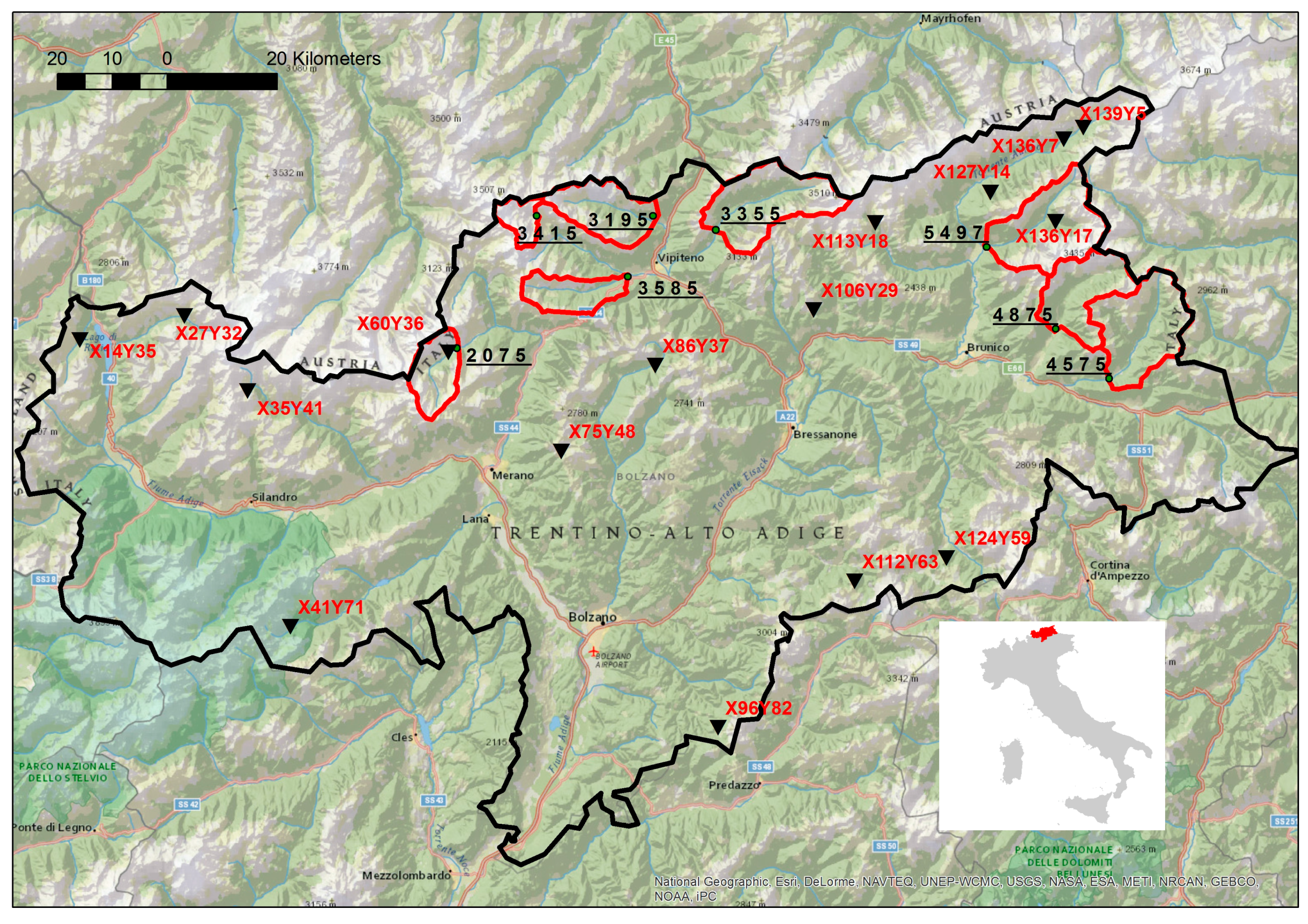
Figure 2.
Examples of scatter plots of estimated and observation-derived snow water equivalent (mm) at selected stations, and corresponding time series. On the right panes, red lines represent model simulations and blue dots represent snow water equivalent (SWE) derived from observed snow depth.
Figure 2.
Examples of scatter plots of estimated and observation-derived snow water equivalent (mm) at selected stations, and corresponding time series. On the right panes, red lines represent model simulations and blue dots represent snow water equivalent (SWE) derived from observed snow depth.
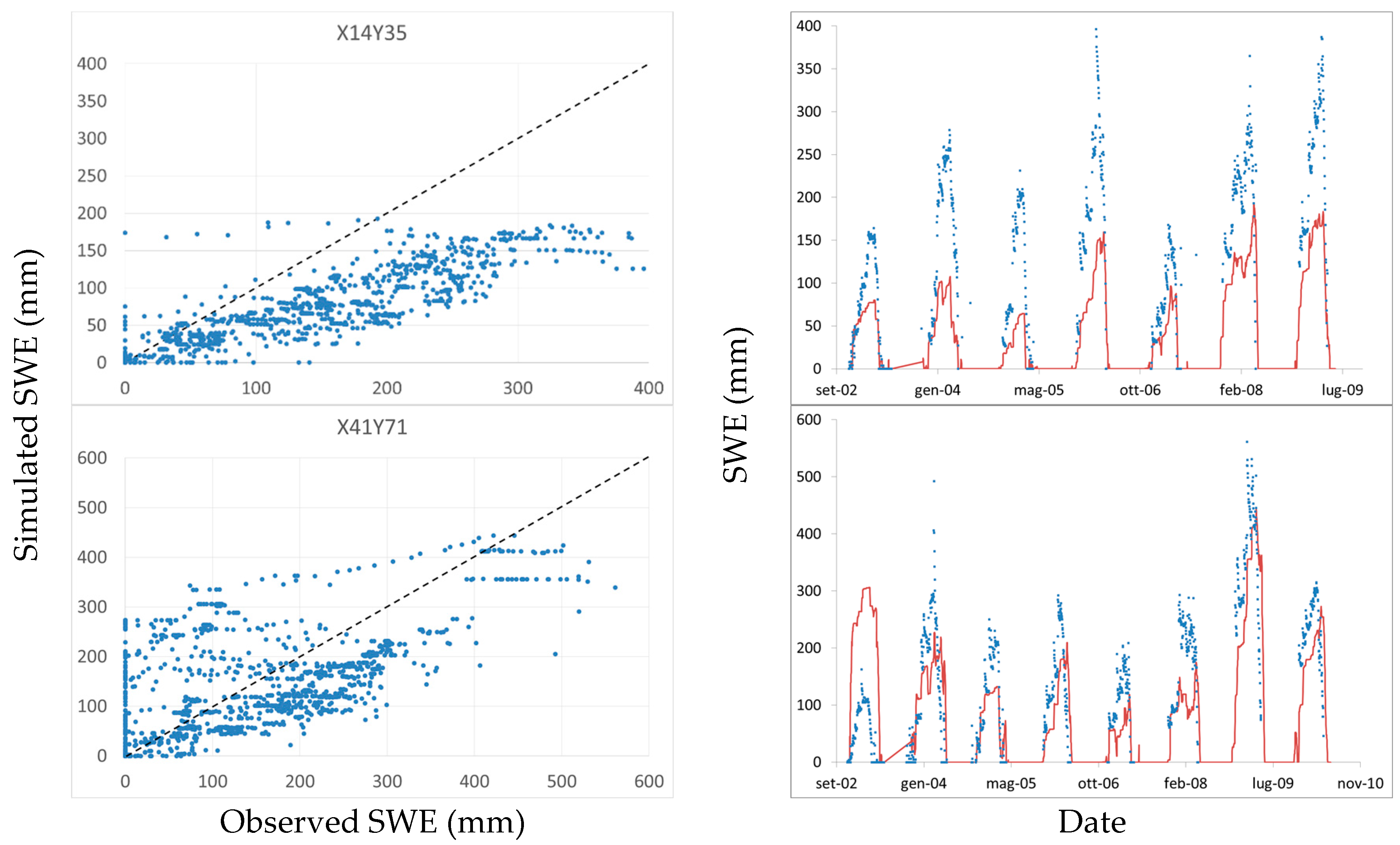
Figure 3.
Comparison of observed discharges and snowmelt. (A) 3415: Vedretta Piana; (B) 4575: Rio Casies a Colle; (C) 4875: Rio Anterselva a Bagni Salomone; (D) 5497: Rio Riva a Caminata; (E) 2075: Rio Plan-Eschbaum; (F) 3585: Rio Racines a Stange; (G) 3355: Rio Vizze a Novale; (H) 3195: Rio Fleres a Colle Isarco. 1:1 lines represented in red with rounded tips.

Table 1.
SNOTEL stations used in the test, and snowmelt coefficients estimated with the proposed approach and in DeWalle et al. [62].
Table 1.
SNOTEL stations used in the test, and snowmelt coefficients estimated with the proposed approach and in DeWalle et al. [62].
| Station | C0 (mm/°C Day) | Average of Daily Snowmelt Coeff. in [62] (mm/°C Day) |
|---|---|---|
| Wolf Creek Summit | 1.79 | 2.9 |
| Beartown | 4.14 | 5.2 |
| Cumbres Trestle | 2.91 | 4.1 |
| Middle Creek | 2.82 | 4.0 |
| Lily pond | 2.87 | 5.9 |
| Culebra #2 | 3.33 | 4.9 |
| Trinchera | 2.03 | 3.2 |
Table 2.
Snow depth measurement stations and explanatory variables (P = cumulative winter snowfall 2002–2010, mm; T = cumulative winter degree-days; P × T = cumulative rain on snow multiplied by daily degree-days; N = cumulative number of days with estimated presence snow cover; N (meas.) = cumulative number of days with snow depth > 0; Z = station elevation; dd = degree-days.
| Code | Station Name | Z (m a.s.l.) | P (mm) | T (dd) | P × T (mm dd) | N | N (Meas.) |
|---|---|---|---|---|---|---|---|
| X136Y7 | Prettau | 1449 | 1386 | 248 | 1914 | 1121 | 1491 |
| X86Y37 | Pens | 1487 | 1068 | 527 | 858 | 818 | 1211 |
| X127Y14 | Klausberg-Steinhaus | 1590 | 1152 | 1456 | 2418 | 1107 | 1432 |
| X139Y5 | Kasern | 1590 | 1349 | 1132 | 2248 | 1039 | 1273 |
| X136Y17 | Rein in Taufers | 1600 | 738 | 660 | 630 | 617 | 1525 |
| X60Y36 | Pfelders | 1620 | 1567 | 1019 | 1845 | 1003 | 1283 |
| X14Y35 | Ausserrojen | 1833 | 1189 | 441 | 532 | 1038 | 1289 |
| X113Y18 | Stausee Neves | 1860 | 1670 | 2484 | 3686 | 1463 | 1351 |
| X96Y82 | Obereggen | 1872 | 1868 | 1125 | 2113 | 1225 | 1056 |
| X41Y71 | Weissbrunn-Ulten | 1890 | 2536 | 727 | 937 | 1273 | 1270 |
| X27Y32 | Melag | 1915 | 1139 | 899 | 1029 | 1050 | 1336 |
| X124Y59 | Piz la Ila | 1995 | 1209 | 2260 | 4480 | 1353 | 1366 |
| X106Y29 | Gitschberg-Meransen | 2010 | 770 | 3088 | 5551 | 1310 | 1554 |
| X75Y48 | Waidmannalm-Hafling | 2040 | 1996 | 2495 | 4462 | 1307 | 1436 |
| X112Y63 | Ciampinoi | 2150 | 2492 | 2048 | 5129 | 1445 | 1190 |
| X35Y41 | Lazauneralm-Schnals | 2450 | 1224 | 2654 | 3155 | 1616 | 1513 |
Table 3.
SWE model performance indicators at the 16 measurement stations. Scatter plots for the stations in bold are presented in Figure 2. Variables are defined in the main text. Nash-Sutcliffe efficiency (NSE); systematic error (MSEs%); unsystematic error (MSEu%); root mean squared error (RMSE).
Table 3.
SWE model performance indicators at the 16 measurement stations. Scatter plots for the stations in bold are presented in Figure 2. Variables are defined in the main text. Nash-Sutcliffe efficiency (NSE); systematic error (MSEs%); unsystematic error (MSEu%); root mean squared error (RMSE).
| Code | NSE | d | R2 | Slope | Intercept (mm) | MSEs% | MSEu% | RMSE (mm) | C0 (mm °C−1 Day −1) |
|---|---|---|---|---|---|---|---|---|---|
| X112Y63 | −3.80 | 0.38 | 0.04 | 0.41 | 98.67 | 9.3% | 90.7% | 201.76 | 1.19 |
| X106Y29 | −1.42 | 0.51 | 0.54 | 0.20 | 2.98 | 98.5% | 1.5% | 217.66 | 0.25 |
| X35Y41 | −0.97 | 0.55 | 0.84 | 0.27 | 4.14 | 99.3% | 0.7% | 216.75 | 0.46 |
| X124Y59 | −0.60 | 0.60 | 0.45 | 0.30 | −0.48 | 92.8% | 7.2% | 168.39 | 0.52 |
| X75Y48 | −0.59 | 0.61 | 0.28 | 0.37 | 35.71 | 77.6% | 22.4% | 157.07 | 0.79 |
| X86Y37 | −0.41 | 0.61 | 0.53 | 0.33 | 6.05 | 93.3% | 6.7% | 140.17 | 1.99 |
| X127Y14 | −0.27 | 0.53 | 0.24 | 0.15 | 41.20 | 94.6% | 5.4% | 163.10 | 0.78 |
| X136Y17 | −0.24 | 0.62 | 0.58 | 0.34 | 23.52 | 93.3% | 6.7% | 131.41 | 1.11 |
| X27Y32 | 0.02 | 0.72 | 0.74 | 0.49 | −4.26 | 91.0% | 9.0% | 94.20 | 1.25 |
| X113Y18 | 0.13 | 0.68 | 0.49 | 0.38 | 24.70 | 83.0% | 17.0% | 126.18 | 0.66 |
| X14Y35 | 0.13 | 0.72 | 0.74 | 0.46 | 9.36 | 91.5% | 8.5% | 87.25 | 2.67 |
| X41Y71 | 0.21 | 0.75 | 0.15 | 0.36 | 70.12 | 57.6% | 42.4% | 102.77 | 3.44 |
| X96Y82 | 0.31 | 0.73 | 0.33 | 0.39 | 56.91 | 56.6% | 43.4% | 78.56 | 1.71 |
| X136Y7 | 0.35 | 0.78 | 0.66 | 0.51 | 30.21 | 79.9% | 20.1% | 97.80 | 5.18 |
| X139Y5 | 0.42 | 0.78 | 0.42 | 0.45 | 52.48 | 52.0% | 48.0% | 71.76 | 1.17 |
| X60Y36 | 0.80 | 0.94 | 0.80 | 0.82 | 12.68 | 17.9% | 82.1% | 40.68 | 1.51 |
Table 4.
Discharge measurement stations used for the testing of snowmelt. The correlation coefficient r is always with p << 1.0E − 05, except for Vedretta Piana where p = 4.6E − 05. Inflow is the average of daily precipitation flows (precipitation times catchment area) during the months of November to May; outflow is the corresponding measured discharge at the catchment outlet. (*) For Station 3415, outflow higher than inflow may be a consequence of the paucity of measurements, not necessarily representative of the average.
| Code | Name | Catchment Area km2 | Elevation m a.s.l. | r | Inflow (m3/s) | Outflow (m3/s) |
|---|---|---|---|---|---|---|
| 2075 | Rio Plan-Eschbaum | 49.6 | 1575 | 0.80 | 1.20 | 1.22 |
| 3195 | Rio Fleres a Colle Isarco | 72.4 | 1063.32 | 0.76 | 5.02 | 1.87 |
| 3355 | Rio Vizze a Novale | 109.7 | 1365.4 | 0.58 | 2.24 | 1.85 |
| 3415 | Vedretta Piana (*) | 23.1 | 2120 | 0.49 | 0.59 | 1.55 |
| 3585 | Rio Racines a Stange | 47.2 | 960 | 0.69 | 2.37 | 1.36 |
| 4575 | Rio Casies a Colle | 117.3 | 1196.07 | 0.71 | 10.74 | 1.65 |
| 4875 | Rio Anterselva a Bagni Salomone | 83.5 | 1095.95 | 0.73 | 8.70 | 1.20 |
| 5497 | Rio Riva a Caminata | 116.2 | 855 | 0.88 | 7.23 | 2.41 |
© 2017 by the authors. Licensee MDPI, Basel, Switzerland. This article is an open access article distributed under the terms and conditions of the Creative Commons Attribution (CC BY) license (http://creativecommons.org/licenses/by/4.0/).
Share and Cite
MDPI and ACS Style
Pistocchi, A.; Bagli, S.; Callegari, M.; Notarnicola, C.; Mazzoli, P. On the Direct Calculation of Snow Water Balances Using Snow Cover Information. Water 2017, 9, 848. https://doi.org/10.3390/w9110848
AMA Style
Pistocchi A, Bagli S, Callegari M, Notarnicola C, Mazzoli P. On the Direct Calculation of Snow Water Balances Using Snow Cover Information. Water. 2017; 9(11):848. https://doi.org/10.3390/w9110848
Chicago/Turabian StylePistocchi, Alberto, Stefano Bagli, Mattia Callegari, Claudia Notarnicola, and Paolo Mazzoli. 2017. "On the Direct Calculation of Snow Water Balances Using Snow Cover Information" Water 9, no. 11: 848. https://doi.org/10.3390/w9110848
Note that from the first issue of 2016, this journal uses article numbers instead of page numbers. See further details here.