An Investigation into Sub-Basin Rainfall Losses in Different Underlying Surface Conditions Using HEC-HMS: A Case Study of a Loess Hilly Region in Gedong Basin in the Western Shanxi Province of China

Abstract

Basins located in loess hilly–gully regions often suffer flood disasters during the flood season. Meanwhile, the underlying surface of the region can increase the rainfall losses, thereby reducing the flood volume. Therefore, the prediction of rainfall losses on the underlying surface is necessary for scientifically and reasonably forecasting the flood volume. The relationship between the rainfall losses and underlying characteristics was investigated and a method for predicting the rainfall losses using HEC-HMS was presented in this paper with a case study in the Gedong basin, a typical loess hilly region of western Shanxi Province in northern China. Results showed that HEC-HMS could be applied to loess hilly–gully regions. The loss computation results suggested that the losses of sub-basins varied with the density of rainfall. The analysis of influences of rainfall losses, including forestland percentage and slope, indicated that the former had a positive impact, while the latter had a negative influence. The impact of forestland percentage is larger than that of slope. Furthermore, with the increase of forestland percentage, its correlation with rainfall losses was enhanced, and the correlation coefficient ranged between 0.64 and 0.84 from the 1970s to the 2010s.

1. Introduction

Rainfall losses, which occur during flood events, play a crucial role in real-time flood forecasting and flood estimation [1,2]. The losses are generated through canopy interception, infiltration, depression storage, evaporation, and evapotranspiration [3]. Rainfall losses by canopy interception are a significant part of hydrological losses from forested ecosystems. Rainfall interception losses mainly rely on the rainfall characteristics, forest structure, and climatic changes governing the rates of evaporation and evapotranspiration during and after rainfall events [4,5]. Infiltration is a major process in flood generation. Infiltration rate is a function of antecedent soil moisture content that decides the magnitude of flood peak and volume [6]. In semi-arid agricultural areas, evaporation and evapotranspiration from the soil have a significant impact on rainfall losses [7]. However, the underlying surface is a paramount factor affecting rainfall losses during flood events. The effect of the underlying surface on rainfall losses is different because of its vegetation, slope, and tillage measures. It is considered that vegetation might prevent rainfall from reaching the surface due to canopy interception and infiltration; the surface slope is large, the flow speed is fast, and its retention time is short, leading to a small infiltration amount. Tillage measures (terrace) change the slope micro-terrain and increase the roughness so that soil moisture infiltration performance changes, thus affecting rainfall losses. In short, the underlying surface can affect the rainfall losses by interception and infiltration in the flood process [8].

In recent years, many studies have been conducted to examine the relationship between rainfall losses and land use type with different models. The Gash model [9] was applied to the basin covered by sugarcane and riparian forest in order to assess the influence of rapid sugarcane canopy changes on rainfall interception losses and explain the main factors determining the rainfall interception losses [10]. The Liu model [11] was used in an experimental multispecies (Acacia mangium, Gliricidia sepium, Guazuma ulmifolia, Ochroma pyramidale, and Pachira quinata) tree plantation in Soberania National Park to predict rainfall interception losses and estimate the water storage capacities of tree boles; the results revealed that the interspecific differences between observed and simulated cumulative interception loss were significant, with Acacia mangium intercepting more rainfall than other species. The Liu model was most sensitive to variations of evaporation rate [12]. In a mixed evergreen and deciduous broadleaved forest, the rainfall interception loss predictions of the revised Gash model were evaluated and the magnitude of gross precipitation and its distribution into interception losses, through fall and stemflow were quantified [13]. In a word, many investigations concerning rainfall losses focused on vegetation interception, while infiltration research was relatively scarce. Gedong basin is a typical loess hilly–gully region; a number of studies in loess hilly–gully regions focus on soil erosion and soil loss. Feng et al. [14] compared the soil and water conservation performances under three single land use types (cultivated land, CL; switchgrass, SG; and abandoned land, AL) and two composite land use types (CL–SG and CL–AL). The results indicated a general trend in the number of runoff and soil loss events for the five land-use types: CL = CL–SG > CL–AL > SG > AL, and the vegetation coverage was the primary factor controlling soil erosion. Zhang et al. [15] analyzed the influences of the thickness of an aeolian sand layer overlying a loess slope on runoff and sediment production processes by eight simulated rainstorms in the Wind–Water Erosion Crisscross Region of the northern Loess Plateau. Zhu et al. [16] combined three sets of plot data (short slope plots, long slope plots, and soil conservation plots) to evaluate the effectiveness of different conservation measures in reducing runoff and soil loss. Yan et al. [17] explored the effect of watershed management practices on the relationship between runoff and sediment by analyses in the hilly–gully regions of the Loess Plateau; the results suggested that a combination of hillslope and gully erosion control practices effectively reduced sediment delivery and erosion. Li et al. [18] determined the effect of different land use types (artificial forestland, native grassland, and artificial grassland) on soil organic carbon and total soil nitrogen by experimental and statistical analysis; the results showed that land use types had great influence on soil organic carbon and total soil nitrogen, and artificial grassland was the optimal choice to mitigate soil carbon and nitrogen loss in the loess hilly–gully region.

In summary, a majority of previous studies in the loess hilly–gully region concentrated on soil loss and erosion; only a few studies have analyzed rainfall losses with a focus on vegetation interception. In the Gedong basin, most rainfall losses are generated through interception and infiltration. Hence the sub-basins’ rainfall losses (interception and infiltration) under different underlying surface conditions are determined in this study by the HEC-HMS model (Hydrologic Engineering Center-Hydrological Model System，U.S. Army Corps of Engineers–Hydrologic Engineering Center，Washington, DC, USA).

At present, the HEC-HMS model has been widely applied to flood simulation [19], flood forecasting [20,21,22], flood frequency analysis [23], flood plain and hazard [24], flood warning [25], and the impact of climate change, land use change, and human activities on runoff [26,27,28,29]. The HEC-HMS model has different methods to calculate the rainfall losses such as Soil and Conservation Service, Green and Ampt, Initial-Constant, Deficit-Constant, Exponential and Soil Moisture Accounting [6]. The Soil and Conservation Service (SCS) Curve Number (CN) loss model estimates precipitation excess as a function of cumulative precipitation, land use, soil cover, and antecedent soil moisture [6]. The CN can reflect the underlying condition of the basin. Considering CN can reflect the underlying characteristics of the basin, the SCS-CN loss method is applied to this study.

The objective of this study is to analyze the relationship between the rainfall losses and underlying characteristics in the hilly–gully loess region. The underlying characteristics include vegetation, soil, slope, and so on. In this study, the SCS-CN loss model is used to calculate the rainfall losses of sub-basins in different underlying surface conditions, and then the relationship between the rainfall losses and underlying characteristics (the percentage of forestland area and surface slope in sub-basins) is analyzed on the basis of rainfall losses calculation results and existing experimental results in the loess hilly–gully region.

2. Study Area

2.1. Meteorology and Hydrology

Gedong basin, with an area of 724.6 km², is located in the western part of Shanxi Province, China (Figure 1). The geographical coordinates are east longitude 111°03′–111°35′, latitude 37°38′–38°11′, about 30 km from east to west, 30 km from north to south. The basin is a typical hilly and gully region of the Loess Plateau. The area of soil erosion is 524 km², and the area of soil and water conservation is 621 km². The climate of the basin is arid and semi-arid warm temperature, the average annual temperature is 8.7 °C, and the average annual rainfall is 517 mm. Rainfall in the basin is rainstorm type, which is characterized by a small area of heavy rain, large intensity, short duration, and the largest rainstorms concentrated in July or August. According to Gedong hydrological station statistics, the average annual runoff is 109 million m³.

2.2. Soil and Land Use

The soil types are relatively simple; most of the study areas are covered with clay loam, sandy loam, and sandy clay. Land use data of the Gedong basin are extracted from remote sensing images, mainly of forest land, grassland, construction land, and cultivated land (the terraces are located on cultivated land); the situation of land use is shown in Figure 2. Through years of comprehensive management of soil and water conservation, the land use efficiency of Gedong basin is significantly changed. From the remote sensing image data, the area of the terrace is 98.48 km², accounting for 13.6% of the basin area. Land use in different stages is shown in

Table 1. Land use information in different stages.

Ages	Forest Land/%	Grass Land/%	Cultivated Land/%	Construction Land/%	Unused Land/%
1980s	43.31	17.26	36.28	0.48	2.67
1990s	46.04	15.66	35.35	0.77	2.18
2000s	50.58	12.28	34.49	1.33	1.32
2010s	60.89	11.53	24.70	2.88	0

.

After 2010, the area of cultivated land accounts for 24.7% of the total area; forestland is the main land use type, accounting for 60.89% of the total area. Compared with the 1980s, the forest land increased by 17.58%, and the cultivated land decreased by 11.58%. From the 1980s to 2010s, part of the cultivated land was turned into forest.

2.3. Surface Slope Characteristics

Slope has a great impact on rainfall losses, runoff, infiltration, soil erosion, and so on. The slope map of Gedong basin is shown in Figure 3.

The minimum slope of the Gedong basin is 0° and the maximum slope of the Gedong basin is 54.76°. The average slope of the 11 sub-basins is 13.53°, the maximum is 14.97°, and the minimum is 12.44°. Figure 4 shows the scatter plot of average slope with the change in basin area. It can be seen that with the increase in basin area, the average slope first increases, then gradually stabilizes; the relationship can be expressed as follows:

Y_{average slope} = 1.6815lnX + 6.6423R² = 0.6877.

(1)

According to the “TD/T1014-2007 second national land survey technical regulations” provisions, the slope can be categorized into five levels; the break points are 2, 6, 15, and 25° [30]. According to this regulation, combined with the actual situation of the basin, the slope is divided into 0–6°, 6–15°, 15–25°, and 25–55°. Figure 5 reflects the percentage of the area under different slopes, varying with the basin area.

It can be seen in the figure that a slope area of 0–6° is about 15% of the total basin area; 25–55° is about 6% of the total basin area; 6–15° and 15–25° area percentages vary from 30% to 50%. When the basin area is less than 75 km², the 6–15° slope area percentage is higher than that for 15–25°; however, when the basin area is greater than 75 km², the 6–15° slope area percentage is lower than that of 15–25°.

Combined with changes in land use, the average slope of cultivated land is 8.93° in the 2010s, and 15.2° in 1980s, and most of the cultivated land with slope > 15° is converted into forest. Returning cultivated land into forest has a great impact on cultivated land with slope > 15° [31,32].

3. Materials and Methods

3.1. Data Collection

The HEC-HMS model was developed by the U.S. Army Corps of Engineers–Hydrologic Engineering Center to simulate rainfall and runoff. It is used in this study to compute the rainfall losses in the sub-basins. Model is composed of basin models, meteorological models, control specifications, and input data components. These components are used to simulate the hydrologic process in a watershed. Basin characteristics such as study area, streams parameters, digital elevation, slope, land use, soil types, and curve number are extracted from ArcGIS [33].

The input parameters used in the model are listed in

Table 2. HEC-HMS model parameters.

No.	Process	Method	Parameter
1	Loss	SCS Curve Number	Initial abstraction (mm), curve number, impervious (%)
2	Transform	SCS Unit Hydrograph	lag time (min)
3	Routing	Muskingum	K (travel time), X (weighting factor)

.

A simulation calculates the rainfall–runoff response in the basin based on input data from the meteorological model. Meteorological data mainly include precipitation and discharge [34]. Precipitation data is obtained from the rainfall stations installed in the study area. In the model, these data are converted into effective precipitation data using the Thiessen polygon method by default (Figure 6). However, compared with spatial interpolation methods, the Thiessen polygon method has some limitations in calculating rainfall [34,35]. The information of temporal and spatial precipitation distribution is significant when selecting data for the model calibration and validation. Discharge data are provided by Gedong hydrological station, which is the only hydrological station at the outlet of the basin.

A total of 18 flood events from 1970 to 2012 were simulated, and a parameter sensitivity analysis was carried out to provide the basis for the next analysis of rainfall loss in each sub-basin under different underlying surface conditions. In this study, land use types in the 1980s (1980–1989), 1990s (1990–1999), 2000s (2000–2009), and 2010s (2010–2012) were obtained from remote sensing images. Due to a lack of remote sensing images in the 1970s, through field visits and access to the relevant literature, the change of land use during the 1970s and 1980s was very small; therefore, in the simulation and calculation process, the land use types of the 1970s were considered similar to those of the 1980s.

In the control specifications, the time period and time step of the simulation run are defined (15 min) [33]. Input data components contain time-series data, paired data, and grid data; these sections are used as boundary conditions or parameters in the model.

3.2. The Simulation of the HEC-HMS Model

The simulation consists of three steps. The first step is watershed delineation. In this step, the basic data such as precipitation, discharge, geological, soil data, land use, and topographic data are entered into the model. After importing the data, the model is calibrated to define the parameters and then these parameters are validated. Model calibration and validation are important to determine the factors that influence the characteristics of the study area. After the above steps are completed, the simulation results are obtained [36,37].

3.3. Rainfall Losses Calculation

In this study, the SCS Curve Number method is applied to calculate the losses in the catchment. This method describes the loss of precipitation by vegetation interception, depression storage, evaporation, evapotranspiration, and infiltration, and indicates whether runoff is generated. The SCS method calculates the precipitation excess as a function of cumulative rainfall, soil cover, land use, and antecedent moisture content [38,39]. The equation is expressed as follows:

$$\mathrm{Q}=\frac{{\left(\mathrm{P}-{\mathrm{I}}_{\mathrm{a}}\right)}^2}{\left(\mathrm{P}-{\mathrm{I}}_{\mathrm{a}}+\mathrm{S}\right)}$$

(2)

where Q is the cumulative rainfall excess, P is the total rainfall, I_a represents the initial abstraction, and S denotes the maximum potential storage. The formula is established when P > I_a.

The initial abstraction can be computed with:

I_a = 0.2 × S

(3)

The maximum potential storage has a relationship with the curve number, which can be computed as follows:

$$\mathrm{S}=\frac{25400-25400\mathrm{CN}}{\mathrm{CN}}\left(\mathrm{cm}\right)$$

(4)

CN (curve number) can be estimated as a function of land use, soil type, and antecedent moisture content in a basin; it comprehensively reflects the characteristics of the basin before precipitation. The CN layer is determined in ArcGIS by utilizing the soil type and land use map. In order to develop the CN layer, the soil map is divided into different hydrological groups such as A, B, C, and D [3,39]. It is found that the CN varies from 57 to 88. The final CN for the sub-catchments is computed using the following formula:

$$\mathrm{CN}=\frac{{\displaystyle \sum }{\mathrm{A}}_{\mathrm{i}}{\mathrm{CN}}_{\mathrm{i}}}{{\displaystyle \sum }{\mathrm{A}}_{\mathrm{i}}}$$

(5)

where Ai represents the drainage area of sub-catchment i and CN_i is the CN of sub-catchment i.

3.4. Direct Runoff Calculation

In this study, the direct runoff in the catchment is calculated by utilizing the SCS Unit Hydrograph. This describes the process of converting the excess rainfall in the catchment into surface runoff. With the progress of precipitation, excess rainfall forms surface runoff along the surface soil into the river, then reaches the sub-basin exports, and ultimately forms runoff. The lag time for SCS unit hydrograph for each sub-catchment is determined as follows [3,40].

The relationship between the peak flow and the peak arrival time of the runoff curve is expressed as follows:

$${\mathrm{U}}_{\mathrm{P}}=\mathrm{C}\frac{\mathrm{A}}{{\mathrm{T}}_{\mathrm{P}}}$$

(6)

where U_p is the peak flow (m³/s), C is the conversion coefficient, A is the drainage area (km²), and T_p is the peak appearance time (h).

The relationship between the time of the arrival peak and the duration of the unit rainfall is

$${\mathrm{T}}_{\mathrm{p}}=\frac{\Delta \mathrm{t}}{2}+{\mathrm{t}}_{\mathrm{lag}}$$

(7)

where Δt is the duration of the unit rainfall (the time interval of the simulation process in the HEC-HMS model) and t_lag is lag time of the peak.

3.5. Flow Routing

The movement of a flood wave through a river reach is described by the Muskingum method. The key to using the Muskingum method is to determine K and X [20,21,41,42]. K and X are calculated as follows:

$$\mathrm{K}=\frac{\Delta \mathrm{L}}{{\mathrm{V}}_{\mathrm{w}}}$$

(8)

$${\mathrm{V}}_{\mathrm{w}}={\mathsf{\beta }\mathrm{V}}_{\mathrm{av}}$$

(9)

$${\mathrm{V}}_{\mathrm{av}}=\frac{1}{\mathrm{n}}{\mathrm{R}}^{\frac{2}{3}}\sqrt{\mathrm{S}}$$

(10)

where K is the spread time of the flood wave through the river reach (s), ΔL is the length of routing (m), V_w is the flood wave celerity (m/s), β is the exponent, V_av is the average velocity (m/s), n is Manning’s roughness, R is the hydraulic radius (m), and S is the bed slope of the channel (m/m) [43,44].

The value of β depends on river characteristics such as channel geometry, slope, and roughness. The rivers in Gedong basin are mostly wide, rectangular channels, so the value of 5/3 for β is obtained from Manning’s equation for a wide rectangular channel where the hydraulic radius is equal to the average depth [43,44].

$$\mathrm{X}=\frac{1}{2}-\frac{{\mathrm{Q}}_0}{2{\mathrm{SPV}}_{\mathrm{w}}\Delta \mathrm{L}}$$

(11)

$${\mathrm{Q}}_0={\mathrm{Q}}_{\min }+0.5\left({\mathrm{Q}}_{\mathrm{p}}-{\mathrm{Q}}_{\min }\right)$$

(12)

where, X is the weighting factor, Q₀ is the reference flow from the inflow hydrograph (m³/s), Q_min is the minimum flow (m³/s), Q_p is the peak flow (m³/s), and P is the bottom width of flow area or average width (m).

4. Results and Discussions

4.1. Model Construction and Simulation

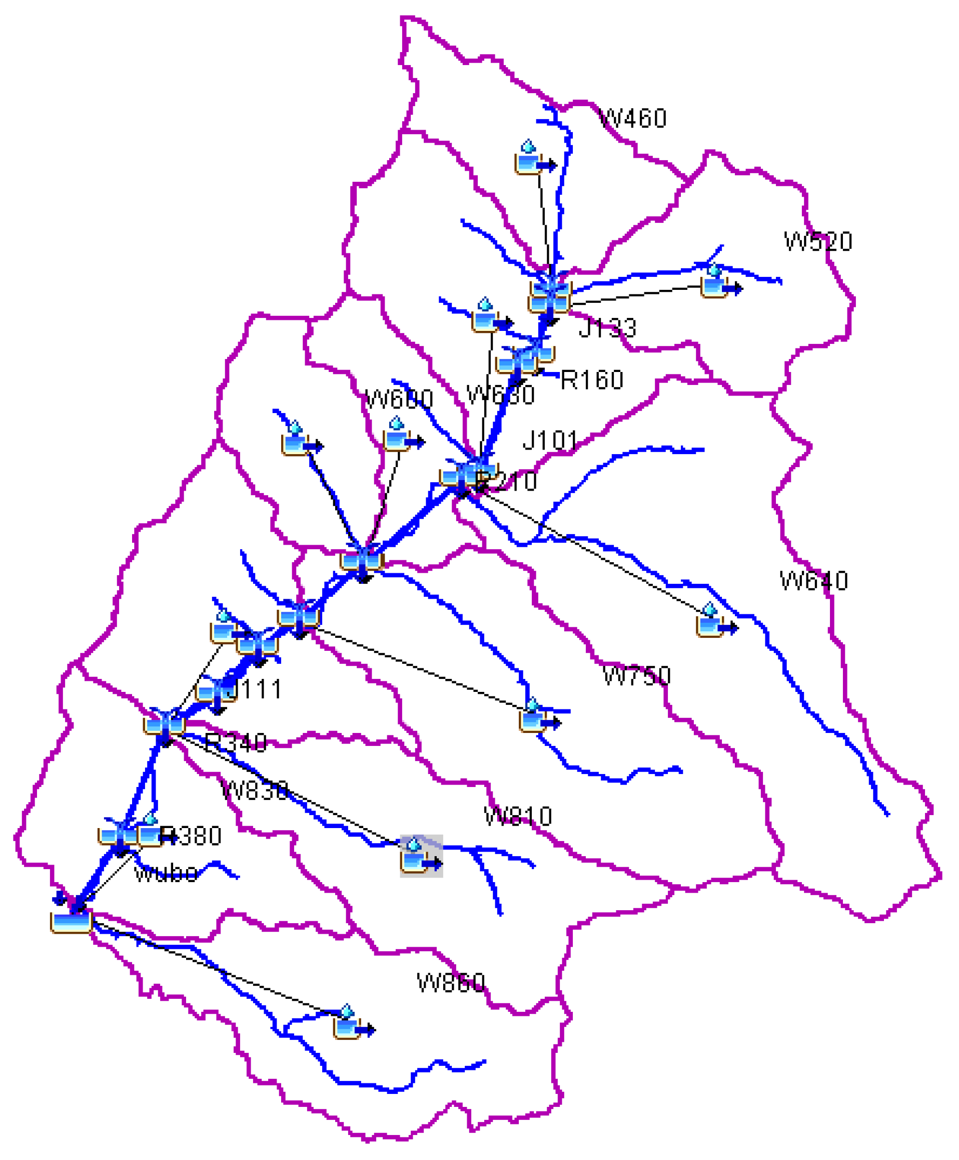
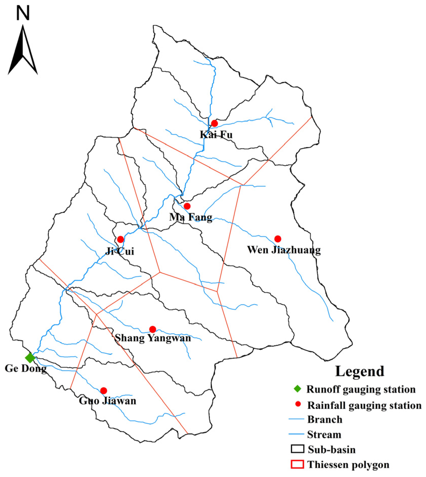
The Gedong basin is divided into 11 sub-basins in order to better represent the spatial variation of parameters. The hydrological model requires that each sub-basin has at least one rainfall node that could represent the sub-basin. In this study, the centroid of the sub-basin was selected as the rainfall node of each sub-basin. The convergence lines of the two sub-basins formed the river channel, until the basin exit section. A generalized model of Gedong basin is shown in Figure 7.

4.2. Sensitivity Analysis

In this study, 18 flood events in different stages were applied to the simulation. A sensitivity analysis was used to examine the relative changes in the model outputs with respect to the change in the model input parameters [41]. Theoretically, if x₁, x₂,…, x_n were model input variables and y = y(x₁, x₂,…, x_n) was the model output, then the relative sensitivity (flexibility) of y with respect to the ith variable at (x₁,…, x′_i,…, x_n) was equal to

$$\mathrm{e}\left(\mathrm{y}\right)=\frac{\partial y}{\partial x_i}\left(x_1,\dots , x_i^{\prime },\dots , x_n\right)\frac{x_i^{\prime }}{y\left(x_1,\dots , x_i^{\prime },\dots , x_n\right)}.$$

(13)

If the absolute value of e was equal to or greater than 1, the model input parameter was flexible. Otherwise, the model input parameter was weakly flexible or inflexible [45,46]. Sensitivity analysis was performed in two stages. The impact of CN (curve number), I_a (initial abstraction), RC (attenuation coefficient), R (peak ratio), K (travel time), X (weighting factor of flow), and t_lag (lag time) on the peak discharge (P) and the impact of CN, I_a, RC, R, K, X, and t_lag on flood volume (V) were assessed in the first and second stages, respectively [46]. The results of the sensitivity analysis are shown in

Table 3. Flexibility coefficients of the model.

Variable	Flexibility	Result	Variable	Flexibility	Result
CN→P	1.21	Flexible	CN→V	1.14	Flexible
Ia→P	−1.12	Flexible	Ia→V	−1.06	Flexible
RC→P	0.01	Inflexible	RC→V	−0.02	Inflexible
R→P	0.40	Inflexible	R→V	0.39	Inflexible
K→P	−1.05	Flexible	K→V	−1.02	Flexible
X→P	0.45	Inflexible	X→V	0.49	Inflexible
tlag→P	−1.08	Flexible	tlag→V	−1.03	Flexible

.

The sensitivity analysis illustrated that CN, I_a, t_lag, and K were sensitive to the peak discharge and flood volume in a loess hilly region such as Gedong basin.

The parameters that were consistent with the flood events of the 1970s and 1980s observed in the hydrograph are shown in

Table 4. Calibrated parameters of 1970s and 1980s.

Parameters	Average Values of Sub-Basins
CN	69.2
Ia	0.3 mm
tlag	66 min
K	0.36

.

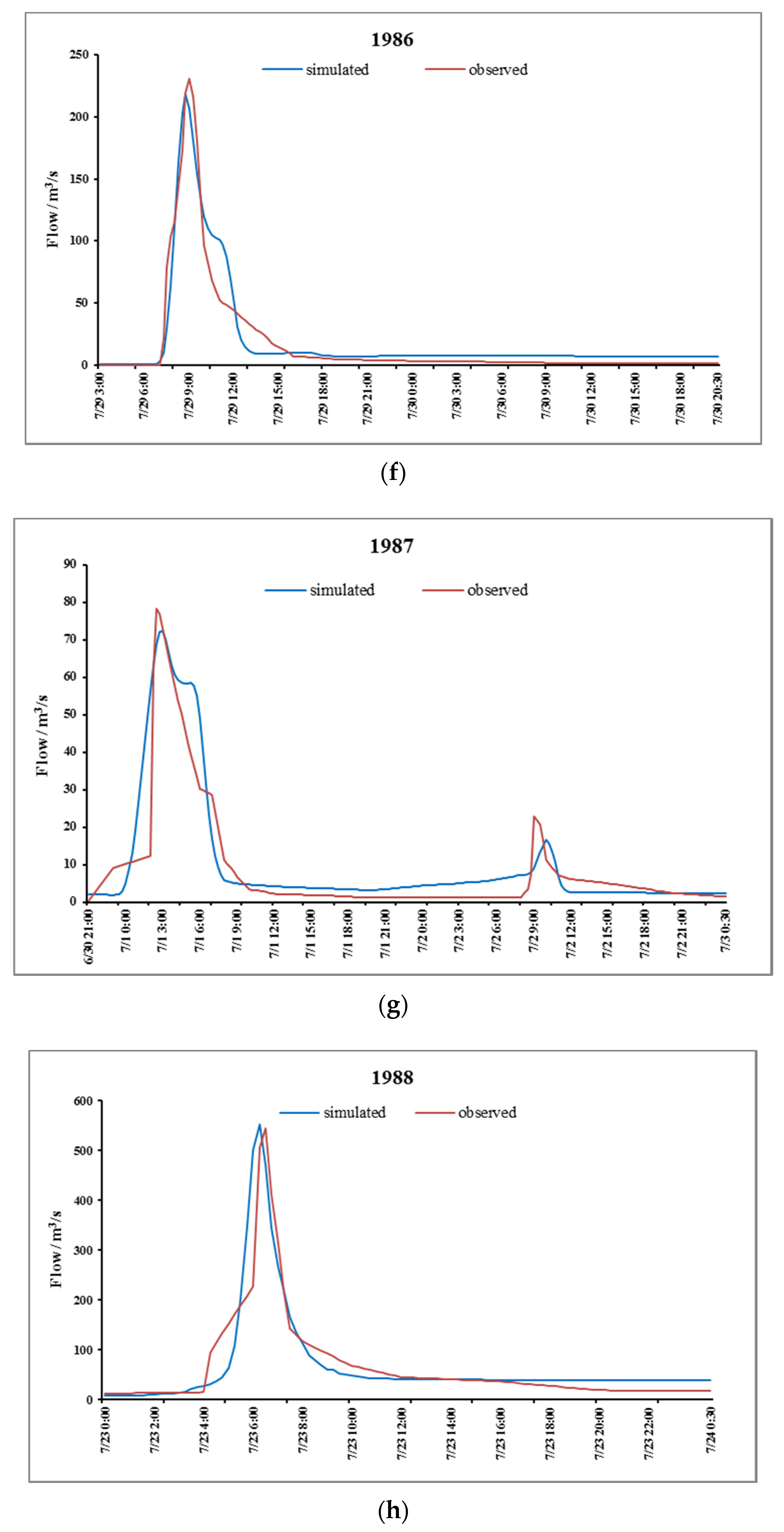
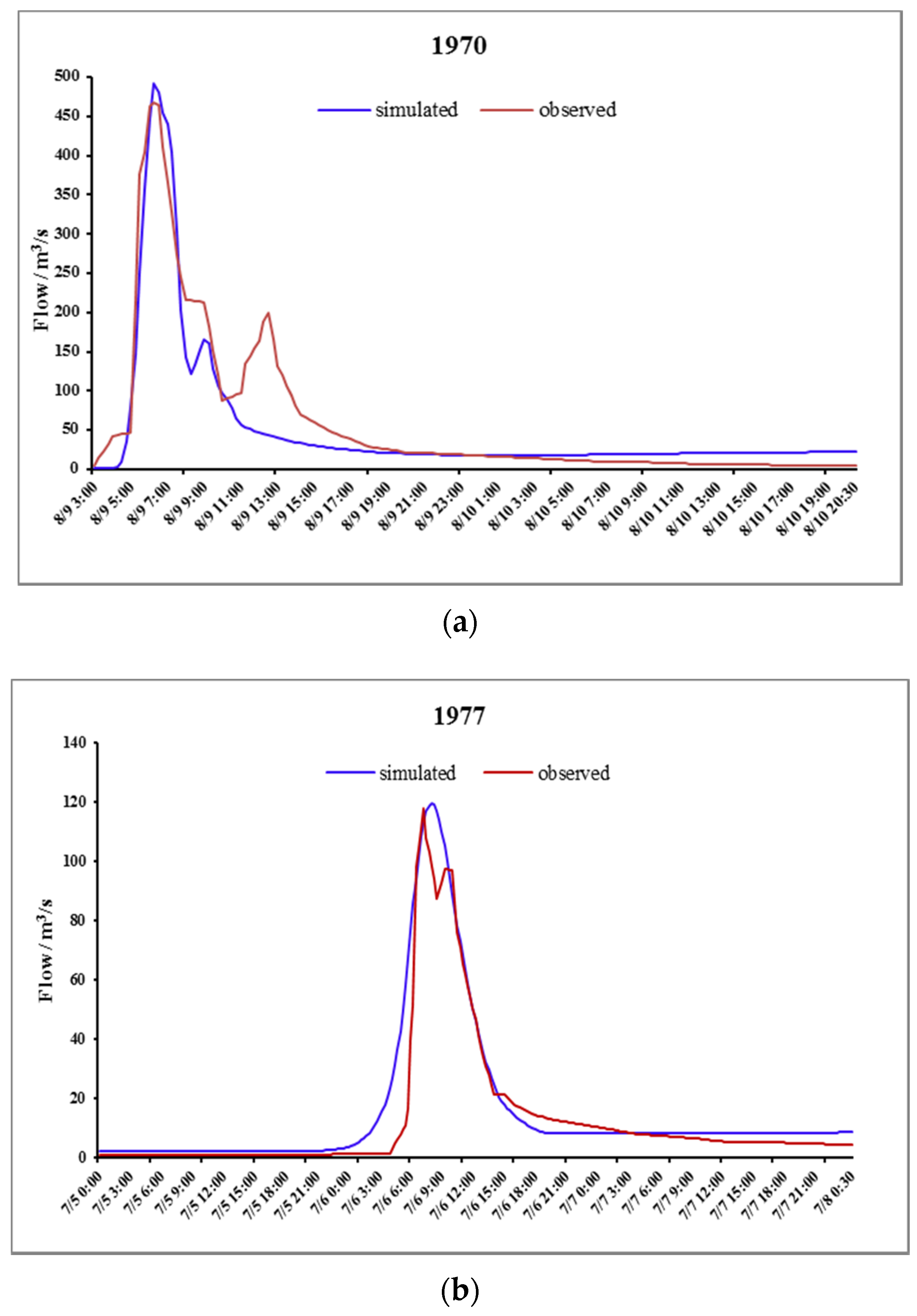
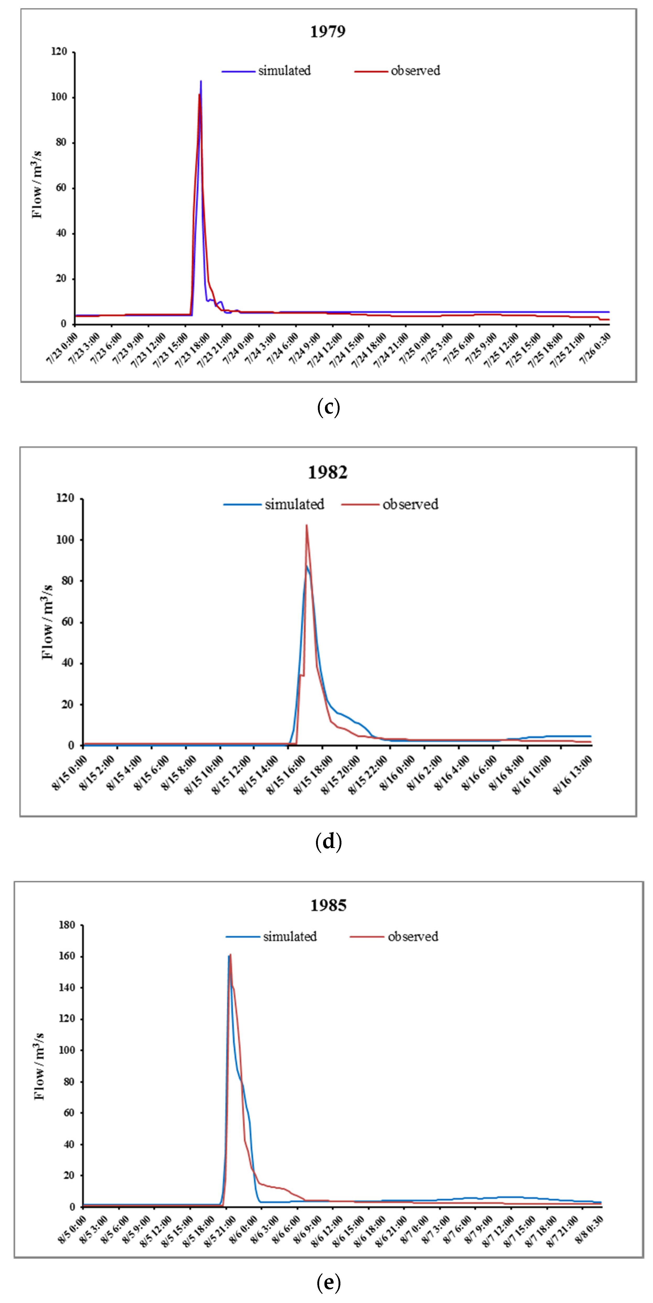
The observed and simulated hydrographs of the 1970s and 1980s are shown in Figure 8.

Overall, the figures described the shape and trend of the hydrographs of eight flood events as being similar, except 1970 and 1977. The total volume was slightly overestimated based on the observed hydrograph in 1977. The peak was slightly underestimated based on the observed hydrograph in 1982, 1986, and 1987, while a relatively perfect match was obtained in 1979.

The parameters that were consistent with the flood events of the 1990s in the observed hydrograph are shown in

Table 5. Calibrated parameters of 1990s.

Parameters	Average Values of Sub-Basins
CN	67.6
Ia	0.34 mm
tlag	68 min
K	0.38

.

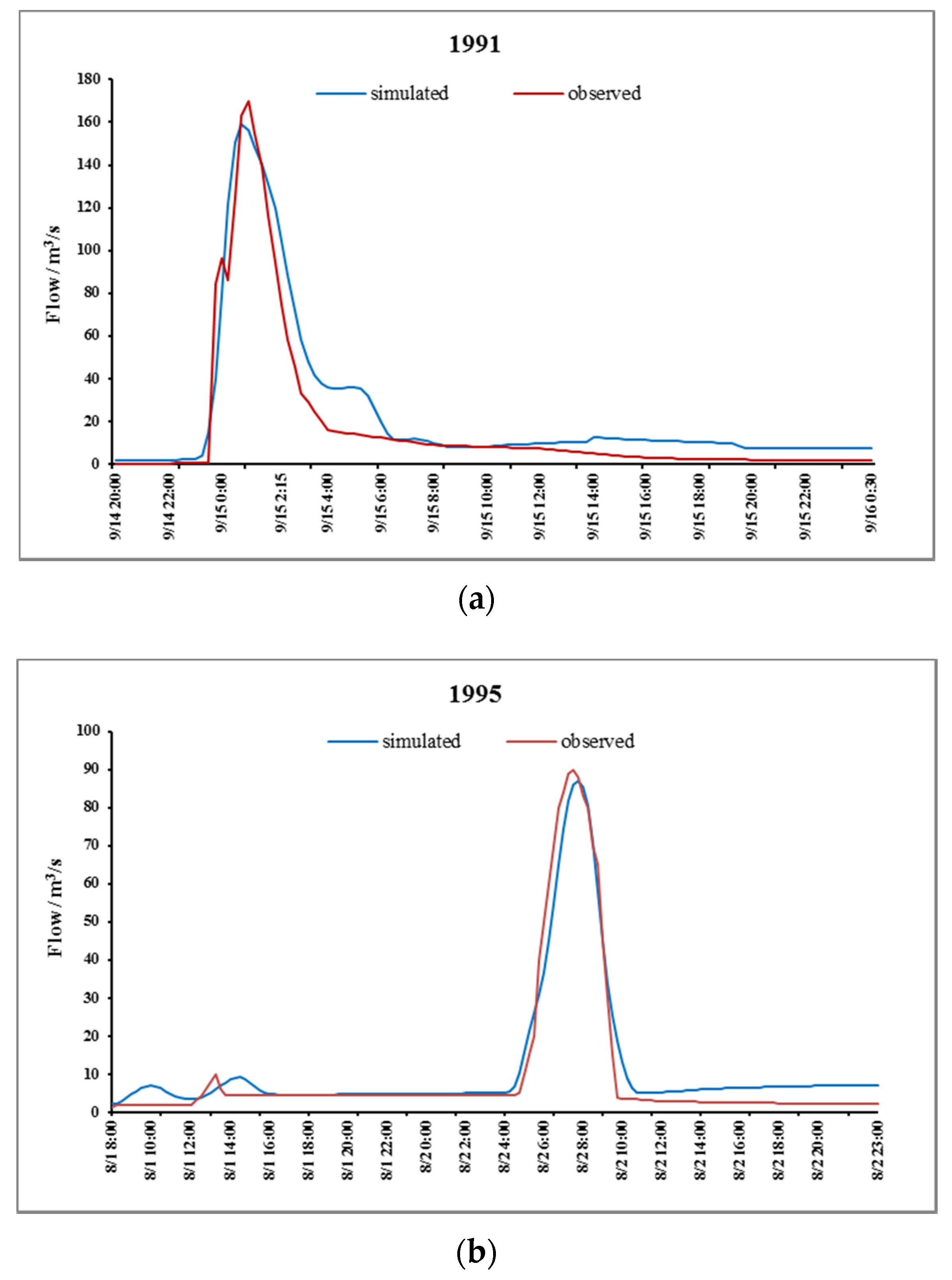
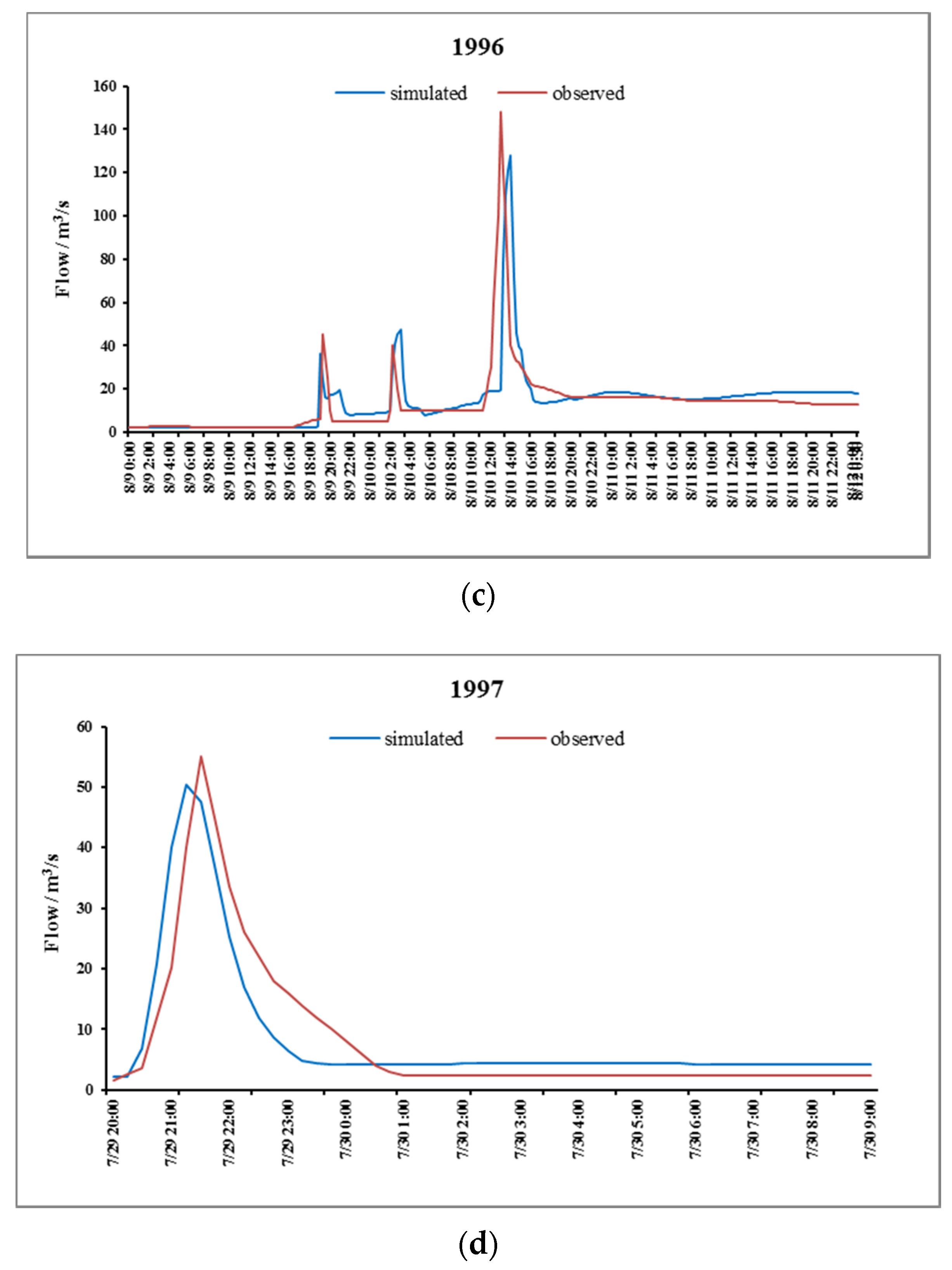
The observed and simulated hydrographs of 1990s are shown in Figure 9.

On the whole, the figures described the shape and trend of the hydrographs of four flood events as being similar. However, the peak of all events was slightly underestimated based on the observed hydrograph.

The parameters that were consistent with the flood events of the 2000s in the observed hydrograph are shown in

Table 6. Calibrated parameters of the 2000s.

Parameters	Average Values of Sub-Basins
CN	64.8
Ia	0.38 mm
tlag	71 min
K	0.43

.

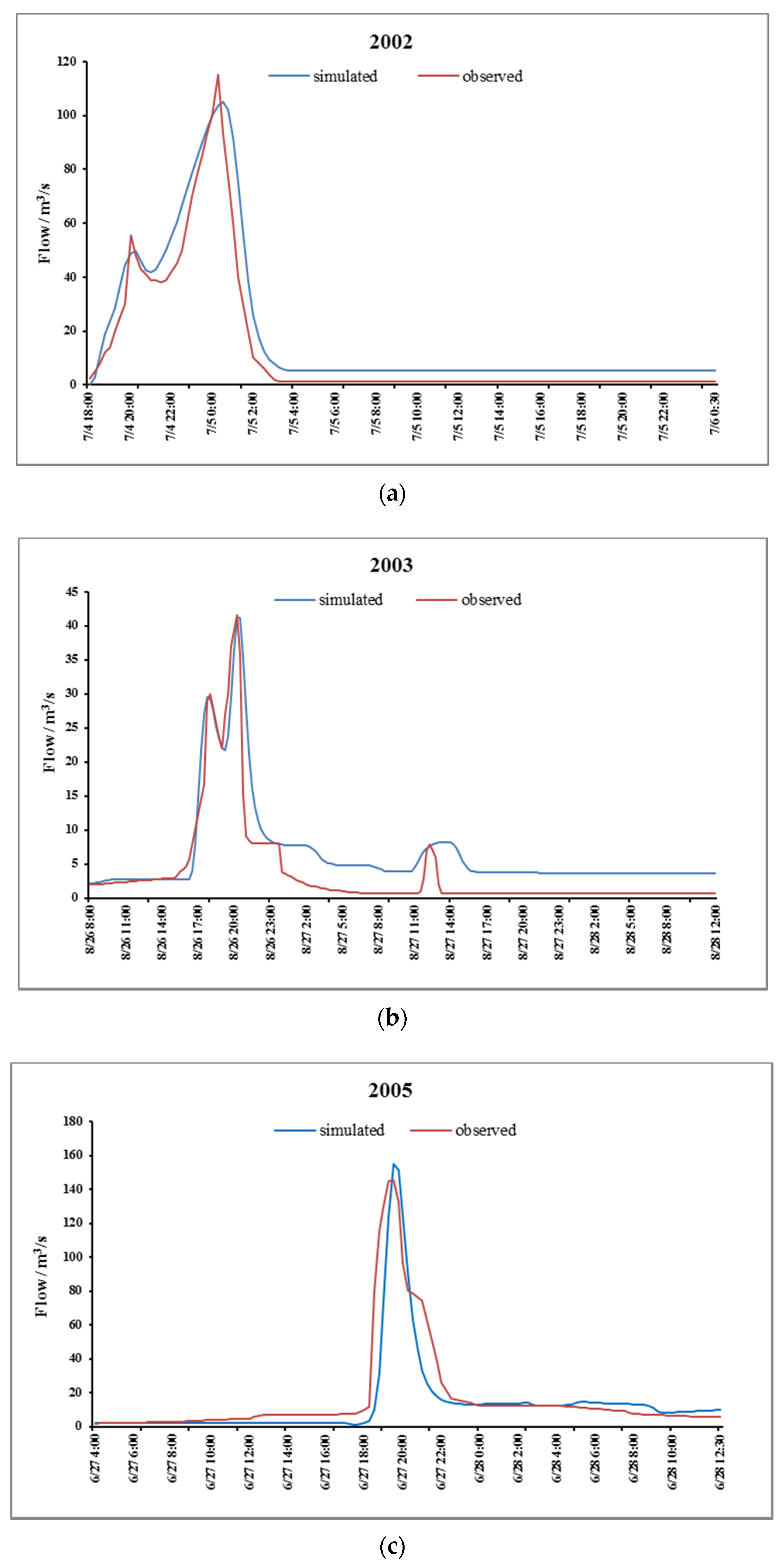
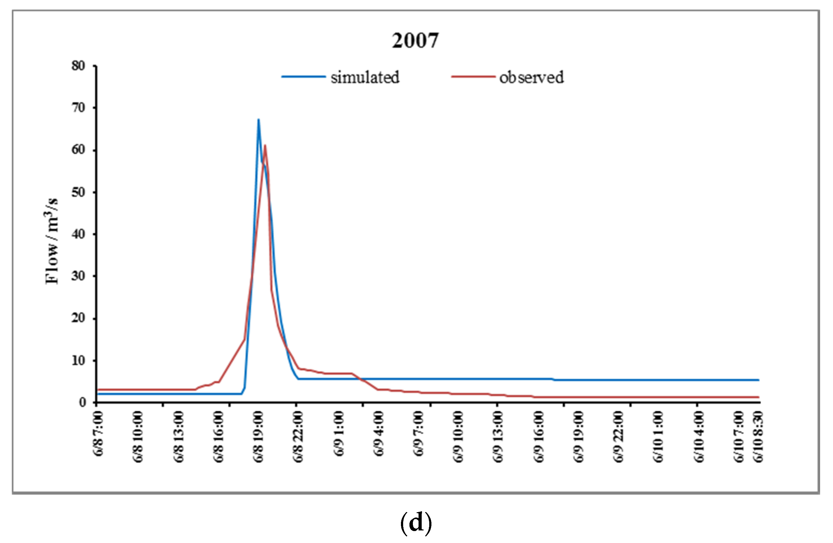
The observed and simulated hydrographs of the 2000s are shown in Figure 10.

In contrast to the hydrographs of the 1970s, 1980s, and 1990s, similar results were obtained in the 2000s. The shape and trend of the hydrographs of four flood events were similar. The total volume was slightly overestimated based on the observed hydrographs of 2002 and 2003. The peak was slightly overestimated based on the observed hydrographs in 2005 and 2007.

The parameters that were consistent with the flood events of the 2010s in the observed hydrograph are shown in

Table 7. Calibrated parameters of the 2010s.

Parameters	Average Values Of Sub-Basins
CN	63.6
Ia	0.39 mm
tlag	75 min
K	0.46

.

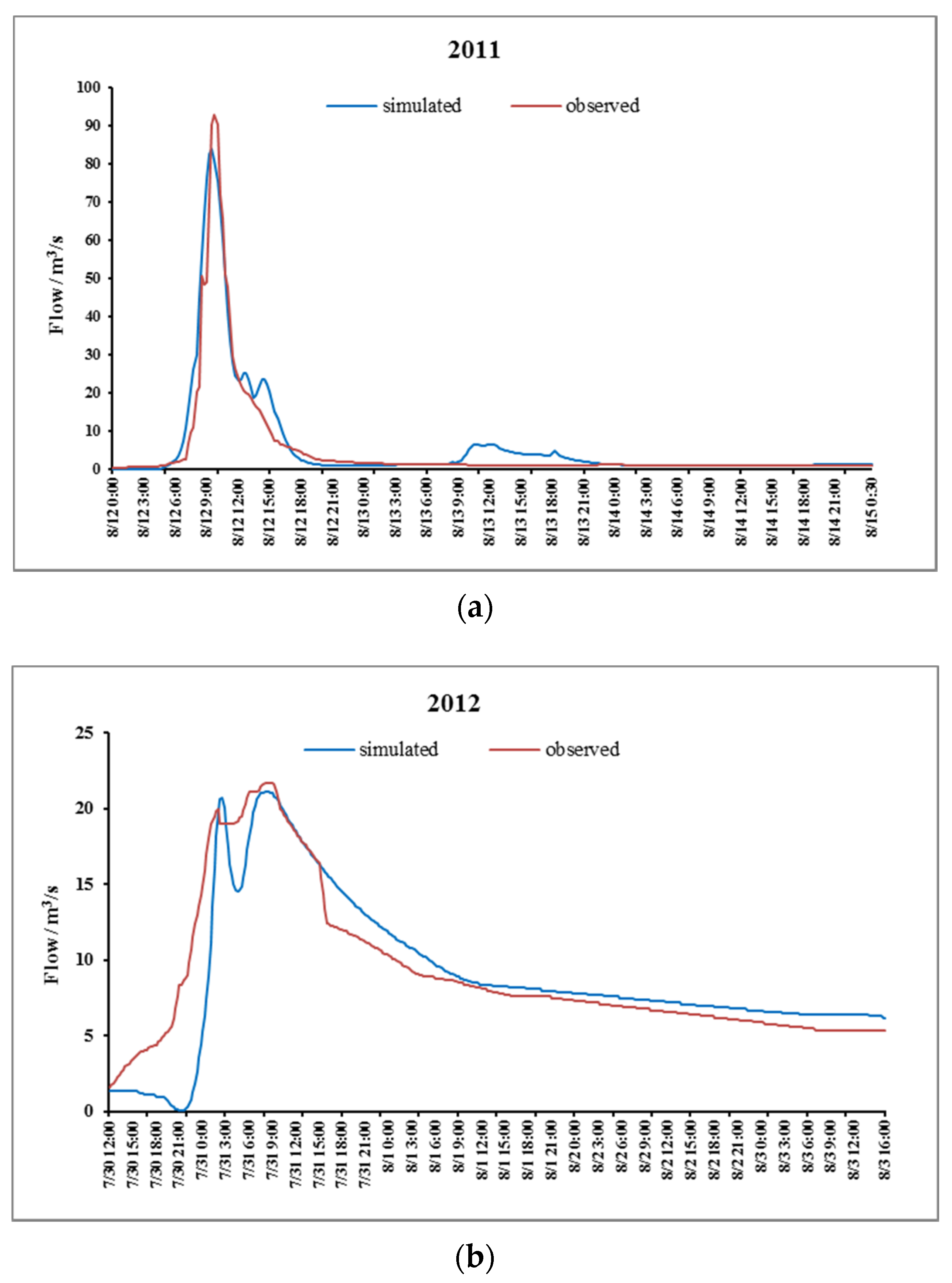
The observed and simulated hydrographs of the 2010s are shown in Figure 11.

It can be seen that the fitness between the simulated and observed hydrographs was less precise than other periods, especially in 2012. This is because, after 2010, the forestland area changed greatly, resulting in great changes of parameters and their underlying characteristics. Moreover, in the SCS model, soil initial moisture was classified into dry, moderate, and wet; such a simple and coarse classification might also lead to increased error during the flood simulation process [6].

Model simulated results and evaluation criteria [47] for 18 flood events are summarized in

Table 8. Simulated results and evaluation criteria.

Flood Events	Observed Peak Discharge/m3/s	Simulated Peak Discharge/m3/s	Peak Flood Error/%	Peak Current Difference/h	Nash Coefficient
19700809	467.50	492.30	5.30	0.00	0.76
19770705	118.00	119.70	1.44	0.75	0.79
19790723	106.60	107.50	0.84	0.25	0.77
19820815	107.10	87.30	−18.49	0.00	0.78
19850805	160.50	161.40	0.56	0.25	0.81
19860729	231.00	218.20	−5.54	0.25	0.71
19870630	78.20	72.50	−7.29	0.50	0.70
19880723	544.00	552.20	1.51	0.25	0.72
19910915	170.00	159.30	−6.29	0.25	0.76
19950801	90.00	80.40	−10.67	0.25	0.74
19960809	148.00	127.70	−13.72	1.00	0.71
19970729	55.00	50.30	−8.55	0.25	0.75
20020704	115.00	105.10	−8.61	0.25	0.79
20030826	41.60	43.90	5.53	0.00	0.70
20050627	145.40	155.00	6.60	0.00	0.78
20070607	61.10	67.30	10.15	0.50	0.76
20110812	93.00	84.00	−9.68	0.25	0.72
20120730	21.70	21.10	−2.76	0.50	0.74

.

It can be seen from Table 8 that the peak flood absolute error between the observed and simulated peak discharge ranged from 0.56% to 18.49%, and the peak current difference ranged from 0 to 1 h. Moreover, the Nash coefficient was higher than 0.7, and the maximum value was 0.81. In summary, the HEC-HMS model was suitable for flood simulation of a loess hilly region in Gedong basin.

4.3. Calculation of Losses in Sub-Basins

Losses in the study area were calculated in the sub-basin for 1972, 1987, 1991, 1996, 2006, and 2012. They represented the underlying characteristics of different ages. The percentage of forestland in each sub-basin and sub-basin area is shown in

Table 9. Sub-basin area and forestland percentage.

Sub-Basin	Area (km2)	Forestland Percentage of 1980s (%)	Forestland Percentage of 1990s (%)	Forestland Percentage of 2000s (%)	Forestland Percentage of 2010s (%)
W810	75.93	56.57	70.43	75.50	79.00
W740	62.36	29.37	32.93	37.61	50.24
W750	101.48	56.94	59.95	67.63	68.44
W630	29.75	29.65	29.01	40.31	48.18
W600	32.97	50.84	51.58	61.89	71.12
W640	133.66	46.83	50.31	64.77	66.32
W530	67.74	33.28	33.49	44.67	52.13
W520	49.30	33.16	34.60	51.57	53.41
W460	41.16	18.38	18.68	28.76	36.71
W860	72.95	60.23	64.13	68.19	73.90
W830	57.30	14.81	21.64	21.00	40.57

.

According to the “Standard for hydrological information and hydrological forecasting (GB/T 22482-2008),” in this work we proposed four model performance classes as a guidance on reference Nash coefficient range, which were denoted as Unsatisfactory (Nash coefficient < 0.5), Acceptable (0.5 ≤ Nash coefficient < 0.7), Good (0.7 ≤ Nash coefficient < 0.9), or Very good (Nash coefficient ≥ 0.9) [48]. The Nash coefficients of 19 July 1972, 30 June 1987, 15 September 1991, 9 August 1996, 14 August 2006, and 30 July 2012 used for the calculation of rainfall losses, as shown in

Table 10. The Nash coefficients of flood events.

Flood Events	Nash Coefficients	Evaluation of Nash Coefficients
19 July 1972	0.68	Acceptable
30 June 1987	0.70	Good
15 September 1991	0.76	Good
9 August 1996	0.71	Good
14 August 2006	0.78	Good
30 July 2012	0.74	Good

.

Table 10 illustrates that the probability of the model fit being considered Unsatisfactory, Acceptable, Good, and Very good was 0%, 16.67%, 83.33%, and 0%, respectively. So the calculation of rainfall losses was feasible.

The results of losses calculation are shown in

Table 11. Basin losses of 1972.

Sub-Basin	Precipitation Volume (mm)	Loss Volume (mm)	Precipitation Volume (1000 m3)	Loss Volume (1000 m3)	% Losses per Sub-Basin
W810	39.90	34.42	3029.69	2613.35	86.26
W740	83.80	68.17	5225.52	4250.73	81.35
W750	49.81	43.73	5054.72	4437.98	87.80
W630	57.30	40.46	1704.90	1203.85	70.61
W600	83.80	68.80	2762.72	2268.19	82.10
W640	44.18	40.19	5905.06	5371.31	90.96
W530	61.54	52.31	4168.60	3543.11	85.00
W520	58.26	43.38	2872.22	2138.32	74.45
W460	62.60	45.32	2576.37	1865.29	72.40
W860	17.84	15.35	1301.43	1119.84	86.05
W830	31.44	22.51	1801.51	1289.88	71.60
Total	590.47	474.63	36,402.72	30,101.84

,

Table 12. Basin losses of 1987.

Sub-Basin	Precipitation Volume (mm)	Loss Volume (mm)	Precipitation Volume (1000 m3)	Loss Volume (1000 m3)	% Losses per Sub-Basin
W810	38.50	33.83	2923.38	2569.07	87.88
W740	68.40	55.73	4265.22	3474.87	81.47
W750	41.43	36.91	4204.32	3746.05	89.10
W630	43.30	30.96	1288.35	921.17	71.50
W600	68.40	56.41	2255.01	1859.71	82.47
W640	35.46	32.26	4739.55	4312.04	90.98
W530	49.78	42.32	3372.00	2866.54	85.01
W520	47.82	36.29	2357.53	1788.89	75.88
W460	51.40	37.26	2115.42	1533.47	72.49
W860	16.36	14.33	1193.46	1045.47	87.60
W830	26.94	19.34	1543.66	1108.35	71.80
Total	487.79	395.64	30,257.89	25,225.62

,

Table 13. Basin losses of 1991.

Sub-Basin	Precipitation Volume (mm)	Loss Volume (mm)	Precipitation Volume (1000 m3)	Loss Volume (1000 m3)	% Losses per Sub-Basin
W810	27.50	25.18	2088.13	1911.97	91.56
W740	32.00	26.84	1995.42	1673.66	83.88
W750	65.12	58.26	6608.38	5912.35	89.47
W630	52.50	37.93	1562.09	1128.61	72.25
W600	32.00	27.09	1054.98	893.25	84.67
W640	111.62	102.14	14,919.02	13,651.75	91.51
W530	62.02	54.10	4201.11	3664.56	87.23
W520	76.80	60.49	3786.24	2982.35	78.77
W460	64.40	46.69	2650.45	1921.57	72.50
W860	37.08	32.73	2704.99	2387.80	88.27
W830	62.04	45.35	3554.89	2598.63	73.10
Total	623.08	516.81	45,125.69	38,726.49

,

Table 14. Basin losses of 1996.

Sub-Basin	Precipitation Volume (mm)	Loss Volume (mm)	Precipitation Volume (1000 m3)	Loss Volume (1000 m3)	% Losses per Sub-Basin
W810	1455.00	50.66	4176.26	3846.72	92.11
W740	68.00	57.34	4240.28	3575.55	84.32
W750	62.30	56.23	6322.20	5705.83	90.25
W630	65.00	46.99	1934.01	1398.14	72.29
W600	68.00	57.85	2241.83	1907.20	85.07
W640	65.00	59.71	8687.84	7980.78	91.86
W530	67.40	58.87	4565.54	3987.60	87.34
W520	67.40	53.62	3322.82	2643.47	79.55
W460	68.00	49.42	2798.61	2033.93	72.68
W860	59.05	53.16	4307.70	3878.34	90.03
W830	61.20	44.90	3506.76	2572.54	73.36
Total	706.35	588.74	46,103.84	39,530.08

,

Table 15. Basin losses of 2006.

Sub-Basin	Precipitation Volume (mm)	Loss Volume (mm)	Precipitation Volume (1000 m3)	Loss Volume (1000 m3)	% Losses per Sub-Basin
W810	56.40	53.55	4282.57	4066.16	94.95
W740	44.00	37.69	2743.71	2350.24	85.66
W750	45.53	43.10	4620.38	4374.12	94.67
W630	42.75	33.38	1271.98	993.29	78.09
W600	44.00	39.03	1450.59	1286.74	88.70
W640	64.56	63.28	8629.03	8458.58	98.02
W530	23.52	21.33	1593.20	1445.03	90.70
W520	19.66	16.71	969.24	823.56	84.97
W460	40.40	30.08	1662.70	1237.88	74.45
W860	64.59	59.87	4711.84	4367.52	92.69
W830	54.36	41.68	3114.83	2388.14	76.67
Total	499.77	439.70	35,050.06	31,791.26

and

Table 16. Basin losses of 2012.

Sub-Basin	Precipitation Volume (mm)	Loss Volume (mm)	Precipitation Volume (1000 m3)	Loss Volume (1000 m3)	% Losses per Sub-Basin
W810	59.00	57.39	4479.99	4357.74	97.27
W740	75.40	65.17	4701.72	4063.81	86.43
W750	57.94	55.16	5879.75	5597.52	95.20
W630	56.20	48.19	1672.17	1433.79	85.74
W600	75.40	71.23	2485.79	2348.18	94.46
W640	53.48	52.78	7148.08	7054.53	98.69
W530	60.04	55.79	4066.99	3779.10	92.92
W520	59.36	52.22	2926.45	2574.45	87.97
W460	61.00	45.48	2510.52	1871.94	74.56
W860	71.21	68.98	5194.77	5031.94	96.87
W830	51.44	40.48	2947.51	2319.73	78.70
Total	680.47	612.87	44,013.74	40,432.71

.

Table 11 demonstrates that the total precipitation volume generated in the whole basin was 590.47 mm and the loss volume was 474.63 mm, with an average percentage of 80.38% per sub-basin. The losses of W630, W520, W460, and W830 were below the average value.

Table 12 showed that the total precipitation volume generated in the whole basin was 487.79 mm and the loss volume was 395.64 mm, with an average percentage of 81.11% per sub-basin. The losses of W630, W520, W460, and W830 were below average.

Table 13 shows that the total precipitation volume generated in the whole basin was 623.08 mm and the loss volume was 516.81 mm, with an average percentage of 82.94% per sub-basin. The losses of W630, W520, W460, and W830 were below average value.

Table 14 shows that the total precipitation volume generated in the whole basin was 706.35 mm and the loss volume was 588.74 mm, with an average percentage of 83.35% per sub-basin. The losses of W630, W520, W460, and W830 were below average value.

Table 15 illustrates that the total precipitation volume generated in the whole basin was 499.77 mm and the loss volume was 439.7 mm, with an average percentage of 87.98% per sub-basin. The losses of W740, W630, W520, W460, and W830 were below average value.

Table 16 shows that the total precipitation volume generated in the whole basin was 680.47 mm and the loss volume was 612.87 mm, with an average percentage of 90.07% per sub-basin. The losses of W740, W630, W520, W460, and W830 were below average value.

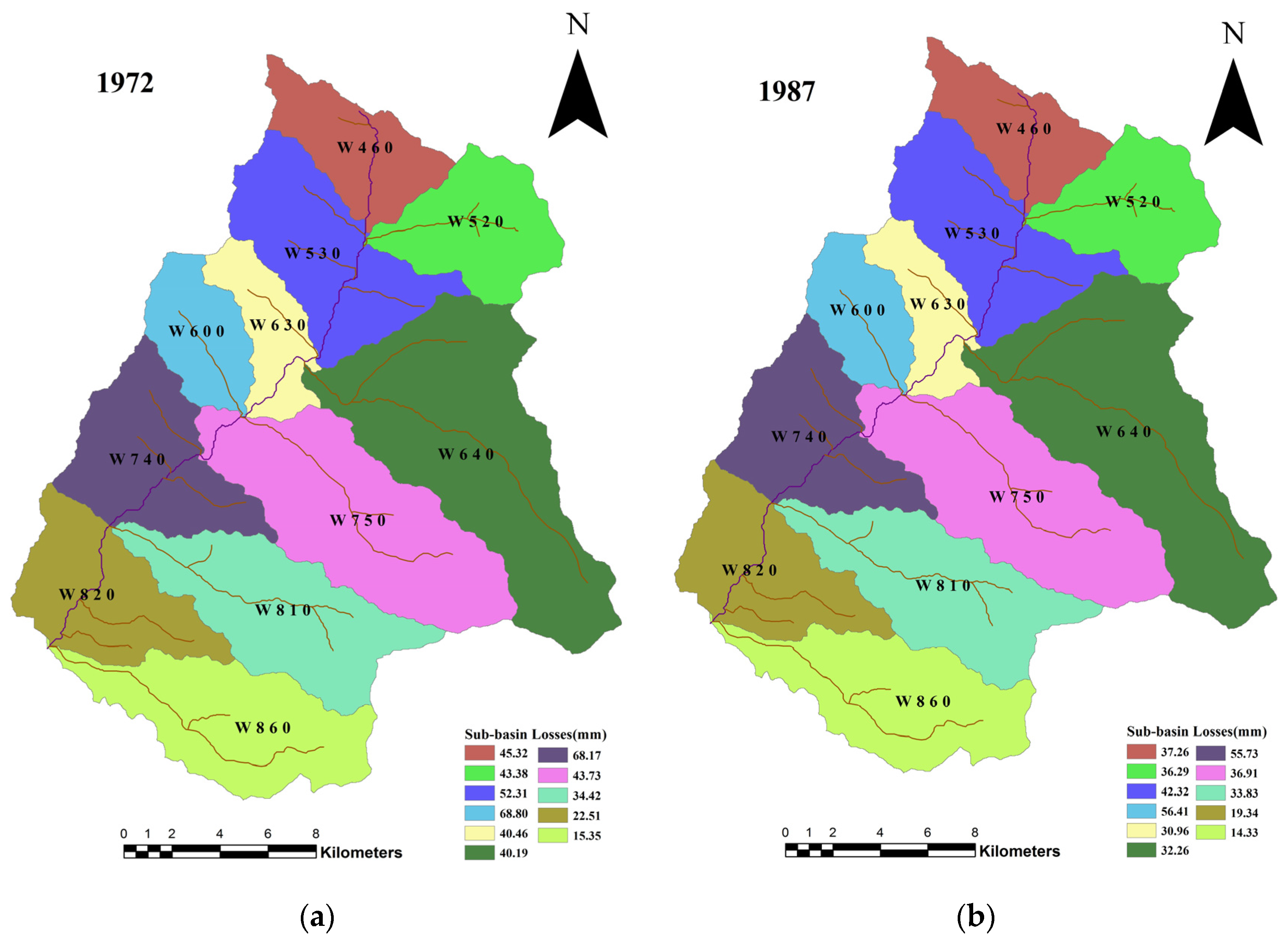
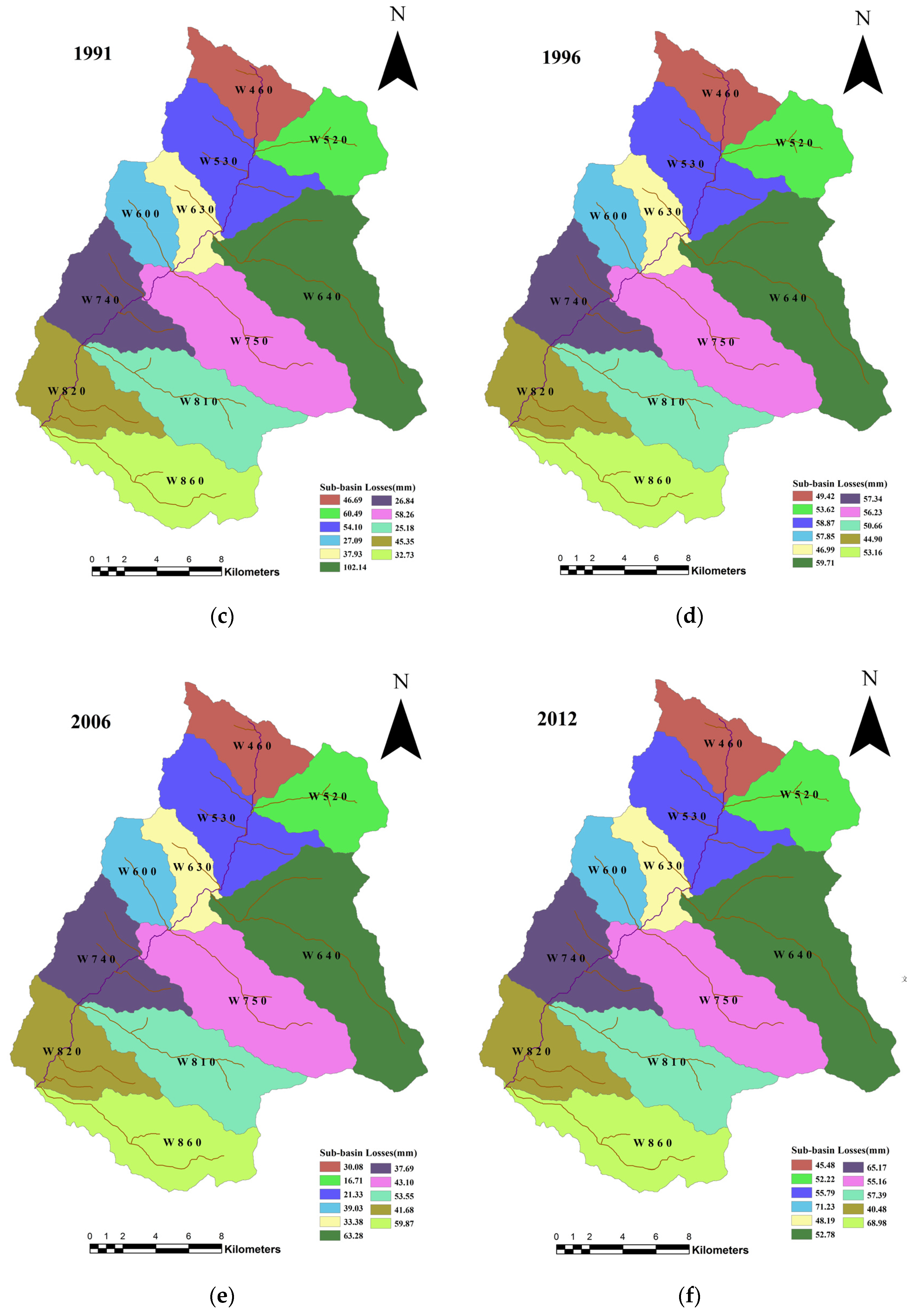
The spatial distribution of the sub-basin rainfall losses is shown in Figure 12.

On the whole, with the increase of forestland percentage, the rainfall losses in the watershed increased from 1972 to 2012. In 1972, the variation range of the rainfall losses of sub-basins was 70.61% to 90.96% and the average percentage of the rainfall losses of sub-basins was 80.38%; in 1987, the variation range was 71.50% to 90.98% and the average percentage of the rainfall losses of sub-basins was 81.11%; in 1991, the variation range was 72.25% to 91.56% and the average percentage of the rainfall losses of sub-basins was 82.94%; in 1996, the variation range was 72.29% to 92.11% and the average percentage of the rainfall losses of sub-basins was 83.35%; in 2006, the variation range was 74.45% to 98.02% and the average percentage of the rainfall losses of sub-basins was 87.98%; in 2012, the variation range was 74.56% to 98.69% and the average percentage of the rainfall losses of sub-basins was 90.07%.

4.4. The Relationship between Rainfall Losses and Forestland Percentage and Slope

According to the experiment in Wangjiagou (a semi-arid hilly loess region of Shanxi Province of China), with an increase of slope angles, the runoff per unit area slightly increased on a short slope (7 m long), but decreased after reaching a maximum at 15° and then decreased with slope angle on a long slope (20 m long), which might be related to the complicated effect of several factors (e.g., rainfall conditions, rill development) on soil infiltrability [16]. In general, with the increase in slope, the rainfall losses gradually decreased. Moreover, for different rainfall periods, about 15° below the slope, slope had a greater impact on infiltration, while a slope greater than 15° had less influence on infiltration [49]. The results revealed that the rainfall losses’ decline was largest at 15°, and the effect of slope on rainfall losses was complex. Thus, rainfall losses were influenced by forestland percentage and slope in Gedong basin. Multiple regression analysis was used to analyze the effects of forestland percentage and slope on rainfall losses in different sub-basins. The results suggested that the effect of forestland on rainfall losses was greater than that of slope, and rainfall losses increased as the forestland percentage increased and slope decreased. The regression equation was as follows:

When the slope was [0, 15°],

y = −0.215x₁ + 0.337x₂ + 81.628 R² = 0.810 Sig. = 0.001.

(14)

When the slope was [15, 55°],

y = −0.021x₁ + 0.520x₂ + 60.585 R² = 0.802 Sig. = 0.000.

(15)

where y represents rainfall losses, x₁ represents the surface slope, and x₂ represents forestland.

As shown in regression Equations (14) and (15), the result of multiple regression analysis was similar to the experimental result in loess hilly regions [49].

4.5. The Impact of Forestland Percentage on Rainfall Losses

In the Wangjiagou basin (a typical loess hilly region), Li Gang et al. [49] obtained the infiltration characteristics of different land types through a rainfall infiltration experiment. The steady infiltration rate of forestland was 0.96–0.99 mm/min, and the steady infiltration rate of cultivated land was 0.39–0.83 mm/min (the higher the slope of cultivated land, the lower the infiltration rate). This indicated that the infiltration rate of forestland was higher than that of cultivated land. So forestland was the main factor influencing rainfall losses in loess hilly regions.

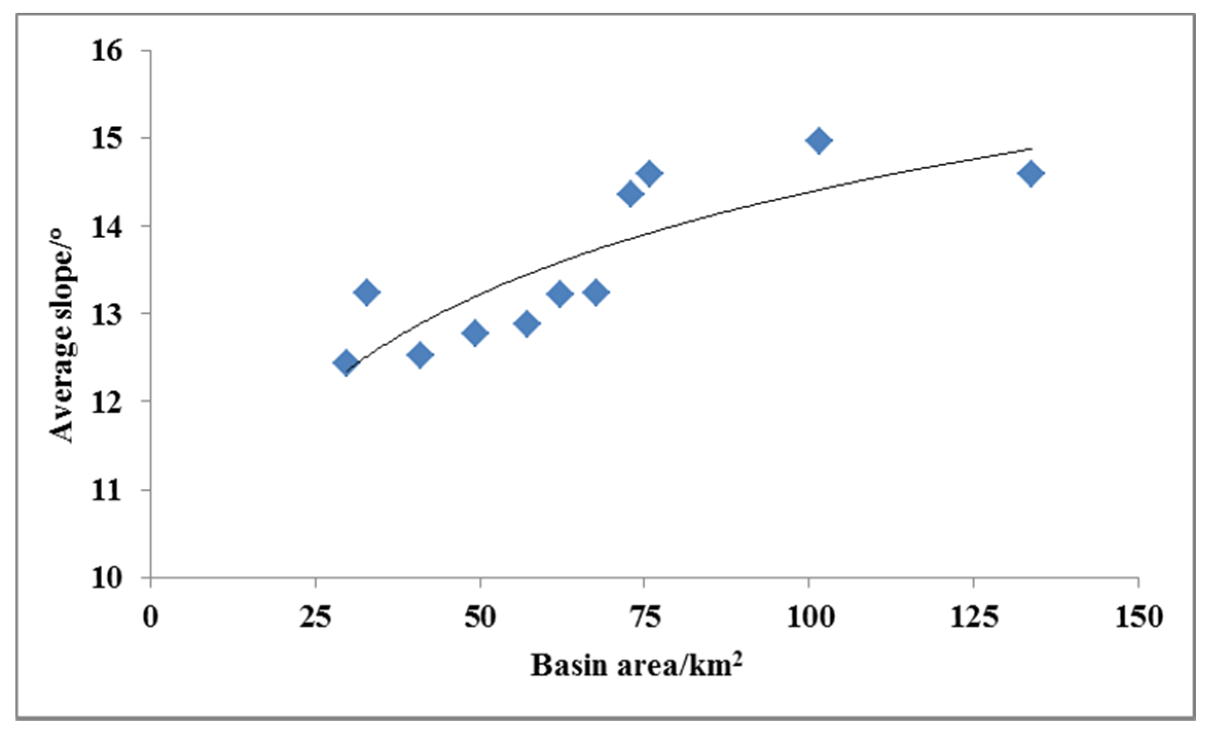
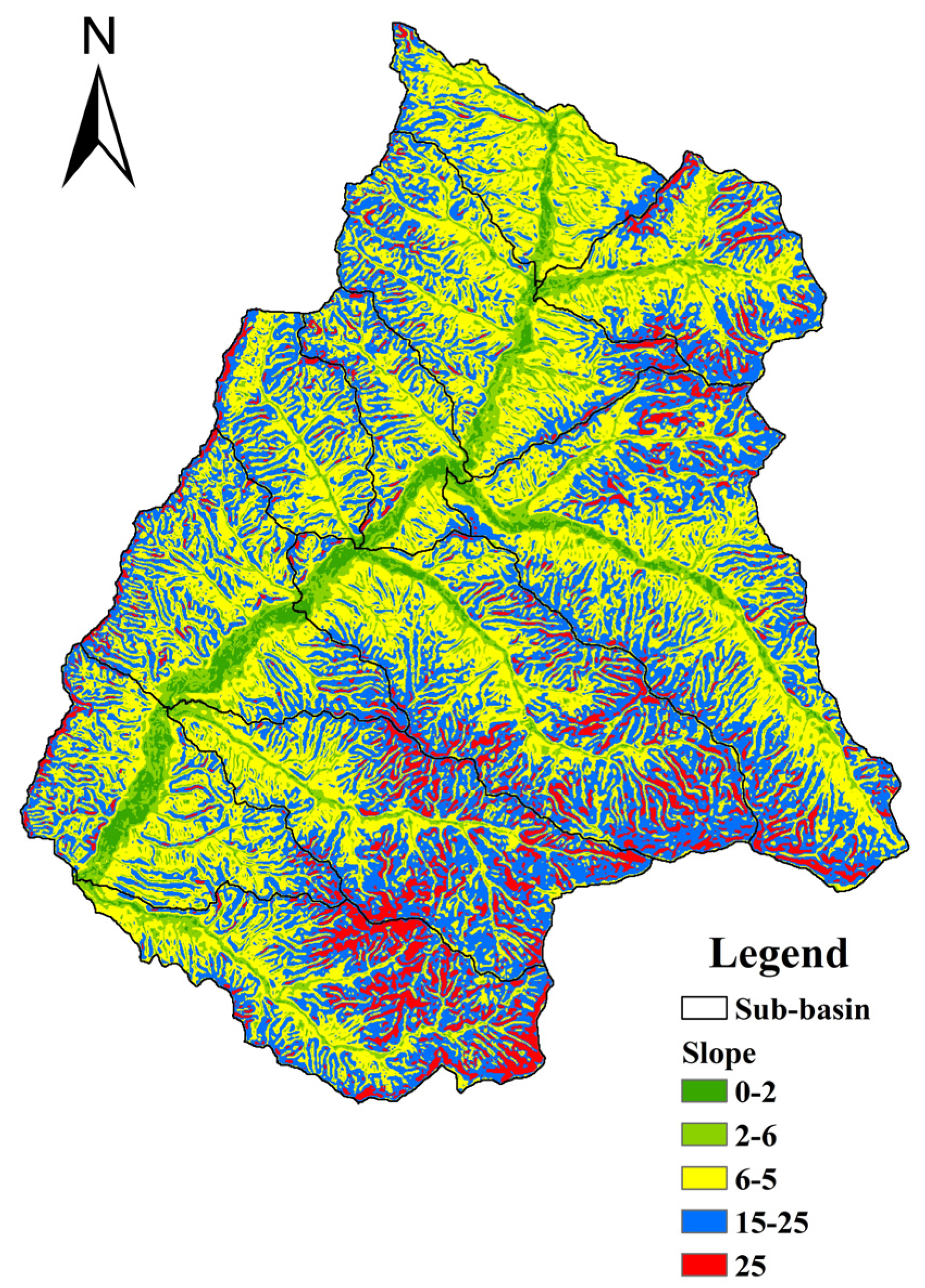
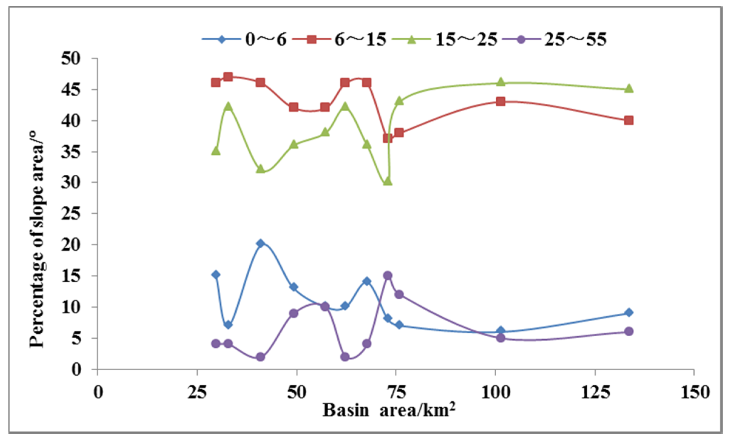
According to the slope analysis, the areas of W740, W630, W520, W460, and W830 were all less than 75 km², so the slope of these sub-basins was mainly 6–15°. In these sub-basins, rainfall losses should be higher than in other sub-basins. However, the losses of W740, W630, W520, W460, and W830 were below the average value in Table 11, Table 12, Table 13, Table 14, Table 15 and Table 16, which was caused by the percentage of forestland in these sub-basins being relatively lower than in others.

The correlation between rainfall losses and percentage of forestland in sub-basins was analyzed under the same rainfall level and different underlying conditions. According to the level of rainfall (30–40 mm; 40–50 mm; 50–60 mm), the flood events were categorized into 19 July 1972 (54.6 mm) and 14 September 1991 (56.4 mm), 30 June 1987 (42.5 mm) and 14 August 2006 (43.6 mm), 9 August 1996 (60.13 mm) and 30 July 2012 (61.61 mm). 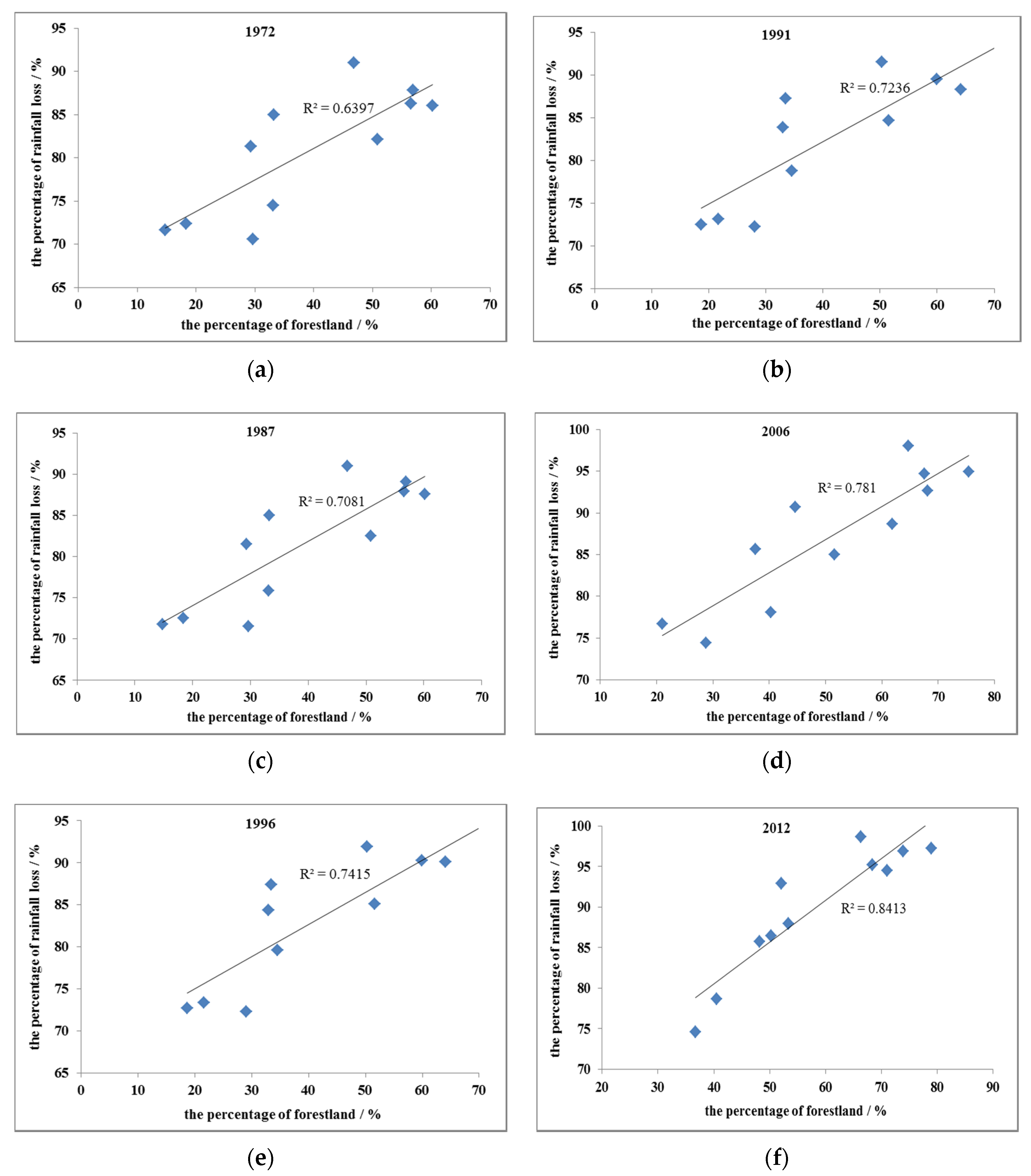In Table 11, Table 12, Table 13, Table 14, Table 15 and Table 16, rainfall losses in 14 September 1991 were 42.18 mm more than 19 July 1972, 14 August 2006 were 44.74 mm more than 30 June 1987, and 30 July 2012 were 24.13 mm more than 9 August 1996, respectively. The results were consistent with the view that the rainfall losses had a positive correlation with forestland percentage. In contrast, the flood volume had a negative correlation with forestland percentage. The information of losses per sub-basin was similar to the information on flood contributing areas. The results of this information were helpful to determine the water availability of different areas. The correlation between rainfall losses and percentage of forestland in sub-basins is shown in Figure 13.

From the 1970s to the 2010s, with the increase of forestland, the correlation coefficient between the percentage of rainfall losses and the percentage of forestland gradually increased. The correlation coefficient of 1972 was lower (0.64). In 2012, the correlation coefficient reached 0.84, which indicates that the rainfall losses of the basin had a positive correlation with the percentage of forestland.

5. Conclusions

This paper presents a case study of the modeling of the rainfall losses and flood processes in a typical loess hilly region in northern China. The SCS–CN model is used to compute the per sub-basin rainfall losses of Gedong basin in HEC-HMS. The model and flood simulation results are validated and compared using observation data from different stages. Losses in the study area are calculated per sub-basin for different stages. The following conclusions can be drawn from the study:

(1)

From the 1970s to the 2010s, when the rainfall was 40–50 mm, the losses of sub-basins were in the range of 71.50%–98.02%; when the rainfall was 50–60 mm, the losses of sub-basins were in the range of 70.61%–91.56%; and when the rainfall was 60–70 mm, the losses of sub-basins were in the range of 72.29%–98.96%.

(2)

In the loess hilly region, rainfall losses are influenced by forestland percentage and slope. Multiple regression analysis suggests that the rainfall losses increase as the forestland area increases and the slope decreases, and the effect of forestland percentage on rainfall losses is greater than that of slope. From 1972 to 2012, with the increase of forestland percentage, the average percentage of rainfall losses in the Gedong basin increased from 80.38% to 90.07%.

(3)

Under the same rainfall level, the rainfall losses are positively correlated with forestland percentage. With the increase of forestland, the correlation coefficient between the percentage of rainfall losses and the percentage of forestland gradually increases. From the 1970s to the 2010s, the correlation coefficient ranged between 0.64 and 0.84.

(4)

Sensitivity analysis indicates that curve number (CN), initial abstraction (I_a), lag time (t_lag), and travel time (K) are the sensitive parameters determining rainfall losses in the basin. The HEC-HMS is appropriate for modeling the flood processes in this typical loess hilly region in northern China. However, the simulation accuracy of the model may be affected by the limitations of the Thiessen polygon method in calculating rainfall. In the future, other spatial interpolation methods such as the Kriging method can be used to calculate the rainfall for improving the simulation accuracy of the model.

References

1. Gamage, S.H.P.W.; Hewa, G.A.; Beecham, S. Modelling hydrological losses for varying rainfall and moisture conditions in South Australian catchments. J. Hydrol. 2015, 4, 1–21. [Google Scholar] [CrossRef]
2. Camici, S.; Tarpanelli, A.; Brocca, L.; Melone, F.; Moramarco, T. Design soil moisture estimation by comparing continuous and storm-based rainfall-runoff modeling. Water Resour. Res. 2011, 47, 1–18. [Google Scholar] [CrossRef]
3. Khalil, U.R.; Khaled, S.B.; Mansour, A.; Amjad, M. Sub-catchments flow losses computation using Muskingum-Cunge routing method and HEC-HMS GIS based techniques, case study of Wadi Al-Lith, Saudi Arabia. Model. Earth Syst. Environ. 2017, 4, 1–9. [Google Scholar]
4. Fan, J.L.; Kasper, T.O.; Adrien, G.; David, A.L. Measuring and modeling rainfall interception losses by a native Banksia woodland and an exotic pine plantation in subtropical coastal Australia. J. Hydrol. 2014, 515, 156–165. [Google Scholar] [CrossRef]
5. Muzylo, A.; Llorens, P.; Valente, F.; Keizer, J.J.; Domingo, F.; Gash, J.H.C. A review of rainfall interception modelling. J. Hydrol. 2009, 370, 191–206. [Google Scholar] [CrossRef]
6. Razmkhah, H. Comparing performance of different loss methods in rainfall-runoff modeling. Water Resour. 2016, 43, 207–224. [Google Scholar] [CrossRef]
7. Nurit, A.; Steven, R.E.; Judy, A.T.; William, P.K.; Paul, D.C.; Joseph, G.A.; Lynn, G.M.; Karen, S.C.; Terry, A.H.; Jose, L.C. Evaporative loss from irrigated interrows in a highly advective semi-arid agricultural area. Adv. Water Resour. 2012, 50, 20–30. [Google Scholar]
8. Saadatkhah, N.; Tehrani, M.H.; Mansor, S.; Khuzaimah, Z.; Kassim, A.; Saadatkhah, R. Impact assessment of land cover changes on the runoff changes on the extreme flood events in the Kelantan River basin. Arab. J. Geosci. 2016, 9, 687–703. [Google Scholar] [CrossRef]
9. Gash, J.H.C.; Lloyd, C.R.; Lachaud, G. Estimating sparse forest rainfall interception with an analytical model. J. Hydrol. 1995, 170, 79–86. [Google Scholar] [CrossRef]
10. Fernandes, R.P.; Silva, R.W.D.; Salemi, L.F.; de Andrade, T.M.B.; de Moraes, J.M.; van Dijk, A.I.J.M.; Martinelli, L.A. The influence of sugarcane crop development on rainfall interception losses. J. Hydrol. 2017, 551, 532–539. [Google Scholar] [CrossRef]
11. Liu, S. Evaluation of the Liu model for predicting rainfall interception in forests world-wide. Hydrol. Process 2001, 15, 2341–2360. [Google Scholar] [CrossRef]
12. Darryl, E.C.M.; Andrew, D.P.; Jessie, L.C. Modelling rainfall interception loss in forest restoration trials in Panama. Ecohydrology 2010, 3, 272–283. [Google Scholar]
13. Su, L.; Zhao, C.M.; Xu, W.T.; Xie, Z.Q. Modelling interception loss using the revised Gash model: A case study in a mixed ever green and deciduous broadleaved forest in China. Ecohydrology 2016, 10, 1749–1758. [Google Scholar]
14. Feng, Q.; Zhao, W.W.; Wang, J.; Zhang, X.; Zhao, M.Y.; Zhong, L.; Liu, Y.X.; Fang, X.N. Effects of different land-use types on soil erosion under natural rainfall in the Loess Plateau, China. Pedosphere 2016, 26, 243–256. [Google Scholar] [CrossRef]
15. Zhang, F.B.; Bai, Y.J.; Xie, L.Y.; Yang, M.Y.; Li, Z.B.; Wu, X.R. Runoff and soil loss characteristics on loess slopes covered with aeolian sand layers of different thicknesses under simulated rainfall. J. Hydrol. 2017, 549, 244–251. [Google Scholar] [CrossRef]
16. Zhu, T.X.; Zhu, A.X. Assessment of soil erosion and conservation on agricultural sloping lands using plot data in the semi-arid hilly loess region of China. J. Hydrol. 2014, 2, 69–83. [Google Scholar] [CrossRef]
17. Yan, Q.H.; Lei, T.W.; Yuan, C.P.; Lei, Q.X.; Yang, X.S.; Zhang, M.L.; Su, G.X.; An, L.P. Effects of watershed management practices on the relationships among rainfall, runoff, and sediment delivery in the hilly-gully region of the Loess Plateau in China. Geomorphology 2015, 228, 735–745. [Google Scholar] [CrossRef]
18. Li, Z.W.; Liu, C.; Dong, Y.T.; Chang, X.F.; Nie, X.D.; Liu, L.; Xiao, H.B.; Lu, Y.M.; Zeng, G.M. Response of soil organic carbon and nitrogen stocks to soil erosion and land use types in the loess hilly-gully region of China. Soil Tillage Res. 2017, 166, 1–9. [Google Scholar] [CrossRef]
19. Knebl, M.R.; Yang, Z.L.; Hutchison, K.; Maidment, D.R. Regional scale flood modeling using NEXRAD rainfall, GIS, and HEC-HMS/RAS: A case study for the San Antonio River Basin, Summer 2002 storm event. J. Environ. Manag. 2005, 75, 325–336. [Google Scholar] [CrossRef] [PubMed]
20. Golian, S.; Saghafian, B.; Maknoon, R. Derivation of probabilistic thresholds of spatially distributed rainfall for flood forecasting. Water Resour. Manag. 2010, 24, 3547–3559. [Google Scholar] [CrossRef]
21. Golian, S.; Saghafian, B.; Elmi, M.; Maknoon, R. Probabilistic rainfall thresholds for flood forecasting: Evaluating different methodologies for modelling rainfall spatial correlation (or dependence). Hydrol. Process 2011, 25, 2046–2055. [Google Scholar] [CrossRef]
22. Haile, A.T.; Tefera, F.T.; Rientjes, T. Flood forecasting in Niger-Benue basin using satellite and quantitative precipitation forecast data. Int. J. Appl. Earth Obs. Geoinform. 2016, 52, 475–484. [Google Scholar] [CrossRef]
23. Haberlandt, U.; Eschenbach, A.D.E.V.; Buchwald, I. A space-time hybrid hourly rainfall model for derived flood frequency analysis. Hydrol. Earth Syst. Sci. 2008, 12, 1353–1367. [Google Scholar] [CrossRef]
24. Zope, P.E.; Eldho, T.I.; Jothiprakash, V. Hydrological impacts of land use-land cover change and detention basins on urban flood hazard: A case study of Poisar River basin, Mumbai, India. Nat. Hazards 2017, 87, 1267–1283. [Google Scholar] [CrossRef]
25. Azam, M.; Kim, H.S.; Maeng, S.J. Development of flood alert application in Mushim stream watershed Korea. Int. J. Disaster Risk Reduct. 2017, 21, 11–26. [Google Scholar] [CrossRef]
26. Hajian, F.; Dykes, A.P.; Zahabiyoun, B.; Ibsen, M. Prediction of climate change effects on the runoff regime of a forested catchment in northern Iran. Hydrol. Sci. J. 2016, 5, 1–22. [Google Scholar] [CrossRef]
27. Lucila, C.; Karim, T.; Gonzalo, O.; Manuel, G. Climate and land use changes on streamflow and subsurface recharge in the Fluvià Basin, Spain. Water 2016, 8, 228–243. [Google Scholar]
28. Noori, N.; Kalin, L.; Sen, S.; Srivastava, P.; Lebleu, C. Identifying areas sensitive to land use/land cover change for downstream flooding in a coastal Alabama watershed. Reg. Environ. Chang. 2016, 16, 1833–1845. [Google Scholar] [CrossRef]
29. Zope, P.E.; Eldho, T.I.; Jothiprakash, V. Impacts of land use—Land cover change and urbanization onflooding: A case study of Oshiwara River Basin in Mumbai, India. Catena 2016, 145, 142–154. [Google Scholar] [CrossRef]
30. Li, H.M. Analysis on the Topographical Characteristics and Vegetation Effects on Runoff Features in the Watershed on Loess Plateau. Master’s Thesis, Beijing Forestry University, Beijing, China, June 2012. (In Chinese). [Google Scholar]
31. Zhang, B.Q.; Wu, P.T.; Zhao, X.N.; Wang, Y.B.; Gao, X.D. Changes in vegetation condition in areas with different gradients (1980–2010) on the Loess Plateau, China. Environ. Earth Sci. 2013, 68, 2427–2438. [Google Scholar] [CrossRef]
32. Wang, C.; Zhen, L.; Du, B.Z. Assessment of the impact of China’s Sloping Land Conservation Program on regional development in a typical hilly region of the loess plateau-A case study in Guyuan. Environ. Dev. 2017, 21, 66–76. [Google Scholar]
33. Kamali, B.; Mousavi, S.J.; Abbaspour, K.C. Automatic calibration of HEC-HMS using single-objective and multi-objective PSO algorithms. Hydrol. Process 2013, 27, 4028–4042. [Google Scholar] [CrossRef]
34. Shi, P.; Rui, X.F. Comparison and improvement of spatial rainfall interpolation methods. J. Hohai Univ. Nat. Sci. 2005, 4, 361–365. (In Chinese) [Google Scholar]
35. Nussaibah, B.R.; Olgu, A.; Necla, T.; Ihsan, C. Space-time kriging of precipitation variability in Turkey for the period 1976–2010. Theor. Appl. Climatol. 2017, 129, 293–304. [Google Scholar]
36. Fares, L.; Rachid, M. Comparison of WBNM and HEC-HMS for runoff hydrograph prediction in a small urban catchment. Water Resour. Manag. 2015, 29, 2485–2501. [Google Scholar]
37. Eyad, A.; Broder, M. Modelling rainfall runoff relations using HEC-HMS and IHACRES for a single rain event in an arid region of Jordan. Water Resour. Manag. 2013, 27, 2391–2409. [Google Scholar]
38. Jin, H.; Liang, R.; Wang, Y.; Tumula, P. Flood-runoff in semi-arid and sub-humid regions, a case study: A simulation of Jianghe watershed in Northern China. Water 2015, 7, 5155–5172. [Google Scholar] [CrossRef]
39. Zema, D.A.; Labate, A.; Martino, D.; Zimbone, S.M. Comparing different infiltration methods of the HEC-HMS model: The case study of the Mésima torrent (southern Italy). Land Degrad. Dev. 2017, 28, 294–308. [Google Scholar] [CrossRef]
40. Yang, Y.M.; Du, J.; Cheng, L.L.; Xu, W. Applicability of TRMM satellite precipitation in driving hydrological model for identifying flood events: A case study in the Xiangjiang River Basin, China. Nat. Hazards 2017, 87, 1489–1505. [Google Scholar] [CrossRef]
41. Andres, G.; Angel, S.; Jose, A.R.; Cesar, A.; Jose, A.J.; Araceli, P. Surface water resources assessment in scarcely gauged basins in the north of Spain. J. Hydrol. 2008, 356, 312–326. [Google Scholar]
42. Homa, R.; Bahram, S.; Ali-Mohammad, A.A.; Fereydoun, R. Rainfall-runoff modeling considering soil moisture accounting algorithm, case study: Karoon III River Basin. Water Resour. 2016, 43, 699–710. [Google Scholar]
43. Kong, F.Z.; Wang, X.Z. Method estimating Muskingum model parameters based on physical characteristics of a river reach. J. China Univ. Min. Technol. 2008, 37, 494–497. (In Chinese) [Google Scholar]
44. Cunge, J.A. On the subject of a flood propagation computation method (Muskingum method). J. Hydraul. Res. 1969, 7, 205–230. [Google Scholar] [CrossRef]
45. Wałęga, A.; Rutkowska, A.; Policht-Latawiec, A. Sensitivity of Beta and Weibull synthetic unit hydrographs to input parameter changes. Pol. J. Environ. Stud. 2014, 23, 221–229. [Google Scholar]
46. Wałęga, A.; Rutkowska, A.; Grzebinoga, M. Direct runoff assessment using modified SME method in catchments in the Upper Vistula River Basin. Acta Geophys. 2017, 65, 363–375. [Google Scholar] [CrossRef]
47. Tak, K.C.; Amin, T.; Sina, A.; Melanie, P.L.O. Choice of rainfall inputs for event-based rainfall-runoff modeling in a catchment with multiple rainfall stations using data-driven techniques. J. Hydrol. 2017, 545, 100–108. [Google Scholar]
48. Ritter, A.; Muñoz-Carpena, R. Performance evaluation of hydrological models: Statistical significance for reducing subjectivity in goodness-of-fit assessments. J. Hydrol. 2013, 480, 33–45. [Google Scholar] [CrossRef]
49. Li, G.; Huang, B.W.; Lu, Z.X. Experimental study on rainfall infiltration-one of the fundamentals of hill slope amelioration in Loess Plateau. Geogr. Res. 1994, 13, 115. (In Chinese) [Google Scholar]
Figure 1. The location and area of Gedong basin.
Water 09 00870 g001
Figure 2. The land use types in Gedong basin.
Water 09 00870 g002
Figure 3. The slope map of Gedong basin.
Water 09 00870 g003
Figure 4. Average slope varying with basin area.
Water 09 00870 g004
Figure 5. Percentage of area under different slopes varying with basin area.
Water 09 00870 g005
Figure 6. Runoff and rainfall gauging station as well as Thiessen polygon in Gedong basin.
Water 09 00870 g006
Figure 7. Generalized model of Gedong basin.
Water 09 00870 g007
Figure 8. Observed and simulated hydrographs of the 1970s and 1980s.
Water 09 00870 g008aWater 09 00870 g008bWater 09 00870 g008c
Figure 9. Observed and simulated hydrographs of the 1990s.
Water 09 00870 g009aWater 09 00870 g009b
Figure 10. Observed and simulated hydrographs of the 2000s.
Water 09 00870 g010aWater 09 00870 g010b
Figure 11. Observed and simulated hydrographs of the 2010s.
Water 09 00870 g011
Figure 12. Sub-basin rainfall losses of the study area.
Water 09 00870 g012aWater 09 00870 g012b
Figure 13. The correlation between the percentage of rainfall loss and the percentage of forestland.
Water 09 00870 g013