BRISENT: An Entropy-Based Model for Bridge-Pier Scour Estimation under Complex Hydraulic Scenarios


1
Department of European and Mediterranean Cultures, Università degli Studi della Basilicata, Potenza 85100, Italy
2
Department of Civil Engineering, Universidad de Concepción, Concepción 4030000, Chile
*
Author to whom correspondence should be addressed.
Water 2017, 9(11), 889; https://doi.org/10.3390/w9110889
Submission received: 21 September 2017
/
Revised: 6 November 2017
/
Accepted: 8 November 2017
/
Published: 14 November 2017
Abstract
:The goal of this paper is to introduce the first clear-water scour model based on both the informational entropy concept and the principle of maximum entropy, showing that a variational approach is ideal for describing erosional processes under complex situations. The proposed bridge–pier scour entropic (BRISENT) model is capable of reproducing the main dynamics of scour depth evolution under steady hydraulic conditions, step-wise hydrographs, and flood waves. For the calibration process, 266 clear-water scour experiments from 20 precedent studies were considered, where the dimensionless parameters varied widely. Simple formulations are proposed to estimate BRISENT’s fitting coefficients, in which the ratio between pier-diameter and sediment-size was the most critical physical characteristic controlling scour model parametrization. A validation process considering highly unsteady and multi-peaked hydrographs was carried out, showing that the proposed BRISENT model reproduces scour evolution with high accuracy.
1. Introduction
Bridges are important for society because they allow social, cultural, and economic connectivity; as such, they are key pieces in the development process and progress. At the same time, bridges continually suffer the action of natural hazards which exposes the road network to risk. The main cause of bridge collapse is related to hydraulic conditions [1,2,3,4,5,6], where flood events can compromise the safety of the whole structure, including its failure. Therefore, the pier-scour phenomenon has become a subject of research for civil and environmental engineers who have proposed many formulas in this field (see e.g., [7,8,9,10]).
Estimating the maximum scour depth around bridge piers and its temporal evolution is a critical step in the design of foundations. Previous researchers have proposed formulas to reproduce the time-dependent scour depth and its maximum value. Among them, Zanke [10] proposed a semi-empirical formulation based on the principle of mass conservation of the bedload. Richardson and Davis [8] used literature data generated by several authors to develop the well-known HEC-18 scour equation, later extended for wide piers. Manes and Brocchini [11] proposed a novel approach combining theoretical arguments with considerations taken from empirical evidence in order to provide new avenues for the development of general predictive models founded more on physical than empirical grounds. Dey [12] elaborated a theoretical model, considering that the key agent in the scour process is the horseshoe vortex. Melville and Chiew [13] and Oliveto and Hager [14] developed empirical scour formulas, where a logarithmic relationship between time and scour-depth was assumed. Subsequently, the Sheppard and Miller [15] and Melville [7] equations were combined and slightly modified in order to form a new scour equation: the Sheppard and Melville (S/M) equation [9]. Although the aforementioned scour models are valid under steady hydraulic conditions, they could be used with stepwise hydrographs adopting the convolution technique (see e.g., [16,17,18,19]). Such technique relies on the superposition concept that allows the consideration of a hydrograph as a sequence of steady discharge steps, in which steady scour models are valid.
Other efforts have been made to explain the bridge scour process under 100% unsteady hydraulic conditions. In this context, Lai et al. [16] examine the rising limb of a triangular hydrograph, introducing an unsteady flow parameter combining peak flow intensity and time-to-peak factors. The effect of a single-peaked flood wave on pier scour was investigated by Hager and Unger [20], who defined the hydrograph by its time to peak and peak discharge. Recently, Pizarro et al. [21] proposed the dimensionless effective flow work parameter for treating bridge scour phenomena under several different hydraulic conditions, showing that multiple peak hydrographs can be analyzed and well represented through . Link et al. [22] proposed the dimensionless effective flow work (DFW) model for evaluating the time-dependent scour-depth under flood waves based on such dimensionless effective flow work.
Furthermore, efforts to monitor real bridge piers have been reported by Sturm et al. [23], Clubley et al. [24], Prendergast and Gavin [25], Hong et al. [26], Su and Lu [27] and others. In particular, Sturm et al. [23] carried out field measurements, laboratory modeling, and 3D numerical modeling of bridge scour. Their field data consisted of a continuous measurement of velocity and scour depth during real flood events, highlighting the scour-hole refilling aspect of the process and the difficulties in scaling the physically modeled scour depth from laboratory to field.
In addition, by applying bridge-scour formulas that take into account constant sediment properties, hydraulic conditions, and pier geometry, the results obtained vary considerably [9]. In this regard, using both field datasets and synthetic data, Gaudio et al. [28] showed that with certain input parameters, different predictions are expected from various bridge scour equations. In another study, Gaudio et al. [29] concluded that the sensitivity of the bridge scour equations to the influencing parameters is not a certain value for all the equations. Hence, various predictions may result using different equations. Therefore, the application of current scour models is restricted to idealized conditions and involves important uncertainties in real cases with complex hydraulic scenarios and natural regimes. Overestimation of scour depth may result in unnecessary costs while, on the other hand, an underestimation imprudently increases the risk of failure of the bridge, loss of life, and connectivity problems. Erosional processes are complex to treat mathematically due to the inherent interaction at different spatial scales. For instance, bridge scour is a local phenomenon that interacts with channel instability, channel bed gradation, channel migration, and contraction scour, which act simultaneously. Consequently, the final response of the bridge depends on the sum of these loads, where the uncertainties of each river process are propagated and accumulated. The issue of quantifying bridge scour uncertainties has already been studied by Barbe et al. [30], Johnson [31,32], Johnson and Ayyub [33,34], Johnson and Hell [35], Johnson and Dock [36], Yanmaz and Cicekdag [37], Yanmaz and Üstün [38], Johnson et al. [39] and others.
Despite previous, enormous efforts, there is still much to do in the field of scour research. For example, recent advances on scour collapse-inducing flow return periods show that their values are considerably scattered, with a range of between one to more than 1000 years [40]. Therefore, linking bridge collapse to a single return period discharge does not provide reliable information on the scour process. Additionally, the potential consequences of climate change on precipitation patterns, catchment characteristics, and river flow characteristics lead to increased uncertainties on bridge scour performances, which are currently unknown.
In this context, informational entropy has long been recognized as a measure of these uncertainties (see e.g., [41,42,43,44,45]) and it is the ideal concept to analyze them in the presence of erosional processes. The goal of this paper is to introduce the first scour model based on both the informational entropy concept and the principle of maximum entropy (POME), showing that a variational approach is ideal for describing erosional processes under complex hydraulic situations.
The paper is organized as follows: first, the informational entropy concept and POME are introduced; the BRISENT model is then formulated and presented in detail; literature data for the model test are described; the calibration/estimation of model parameters is presented and discussed; and the BRISENT model is validated with multi-peaked hydrographs containing sequences of flood events. Conclusions are drawn at the end.
2. The Informational Entropy Concept
The informational entropy concept and its theory have been applied before in statistical mechanics, information theory, hydrology, and water resources (e.g., [46,47,48,49,50,51,52,53]), providing good results and an easy way to introduce probabilities into hydraulics. Informational entropy, Shannon entropy or simple entropy is defined in terms of probability. Taking into account the continuous random variable X, entropy is defined as:
in which is the entropy, is the probability density function of , and denotes expectation. Note that for random variable notation, the Dutch convention is adopted [54] according to which a random variable is underlined.
Informational entropy may be considered a measure of the uncertainties as well as a quantity of information contained in the data [43]. Theoretically, a uniform probability distribution maximizes the entropy defined in Equation (1) [47]; however, due to the constraints that define the physics of different phenomena, the probability density function is not always uniform. According to Chiu [47], the entropy concept can be thought of as a measure of how close the real probability density function is to the uniform function. Therefore, a maximization of entropy will make the probability density function as uniformly as possible, considering the constraints. In this context, and from a physical perspective, the tendency toward maximal entropy is the driving force of natural change, where POME is the logic counterpart of the second law of thermodynamics [43,46].
The maximization of entropy to determine may be resolved using the method of variational calculus. Maximizing Equation (1) and satisfying the “n” constraints defined in Equation (2) is equivalent to maximizing the Lagrange function presented in Equation (3):
in which are the Lagrange multipliers and is the number of constraints. Thus, the mathematical function of can be obtained by solving Equation (4) and therefore, a simple function of can be deduced,
3. The BRISENT Model
The dimensionless, effective flow work by the flow on the streambed around a pier, , was deduced from dimensional analysis and physical considerations by Pizarro et al. [21]:
where is the considered time, is a reference time , is a reference length ( is the pier-diameter and the sediment-size), u is the section averaged flow velocity, is a reference velocity (, where is the relative density between sediment “s” and water “w”, and g is the gravitational acceleration). is the critical flow velocity for incipient motion of sediment particles. Based on experimental evidence (e.g., [10,55,56,57]), it is considered that scour occurs when , thus:
is an energetic parameter applied to local scour phenomena. Consequently, POME applied to results in a variational/thermodynamic approach for treating the local scour process.
Pizarro et al. [21] evidenced that under constant sediment properties, geometrical scale, and clear-water conditions the mathematical relation between the relative scour depth and W* is unique. is defined as a normalized parameter, where z is the dimensional scour depth and the reference length established previously. In agreement with Link et al. [22], increases monotonously over , taking values from zero at non-eroded conditions to a maximum value at the equilibrium state. Based on the Laplace principle of insufficient reason and therefore, assuming that all values of between zero and a maximum considered value, are equally likely to be attached (not necessarily true), then the probability of the relative scour depth to be equal to or less than , , can be specified by . Thus,
and the probability density function of is the derivative of Equation (7):
Unfortunately, Equation (8) cannot be used to determine because the derivate of over is unknown. However, POME can be exploited for this purpose. Equation (9) reveals the informational entropy applied to the scour phenomenon:
Resolving the issue to find the probability density function of implies using Equation (9) with a few constraints that completely define the boundary conditions and physics. The first constraint must satisfy the axiom of probability:
and the second constraint, related to the mass conservation law for bridge-pier scour phenomenon at equilibrium condition, can be written as:
in which is the (W*-averaged) mean relative scour depth, i.e., the average value of Z* during the scour process.
The scour entropy given by Equation (9) needs to be maximized subjected to the constraints in Equations (10) and (11). For this purpose, the method of Lagrange multipliers is adopted. The probability density function is:
where and are Lagrange multipliers. After substitution of Equation (12) into the constraint equations, and considering the boundary condition at , the final equations after some algebra are:
in which is the maximum relative scour depth associated to the maximum dimensionless, effective flow work , is a Lagrange multiplier that needs to be estimated, and is defined as the entropic-scour parameter. Note that due to the physical relationship between and , the BRISENT model contains two fitting parameters: and . These parameters depend on scour influencing parameters and can be estimated as described in the following sections.
4. Methods
4.1. Data Characterization for λ Estimation
Experimental data were compiled from available studies in Chabert and Engeldinger [58], Zanke [10], Franzetti et al. [59], Oliveto and Hager [14,19], Sheppard et al. [60], Grimaldi [61], Alabi [62], Simarro et al. [63], Meyering [64], Lança et al. [65], Link et al. [22] and Pizarro et al. [21]. Altogether, results corresponding to 137 experiments were analyzed. Experimental conditions of scour experiments are presented in Table 1 in which is the experimental time, is the dimensionless particle diameter, is the kinematic viscosity, is the ratio between pier-diameter and sediment-size, is the ratio between flow-depth and pier-diameter, and is the flow intensity.
Note that for run names a standard notation was selected in order to provide a simple and characteristic code that contains the year of publication, author names, number of experiment, and its hydraulic conditions. For example, “2017PIZARRO05U” is the unsteady experiment number 5 carried out by Pizarro et al. [21] and “2004SHEPPARD04S” is the steady experiment number 4 performed by Sheppard et al. [60].
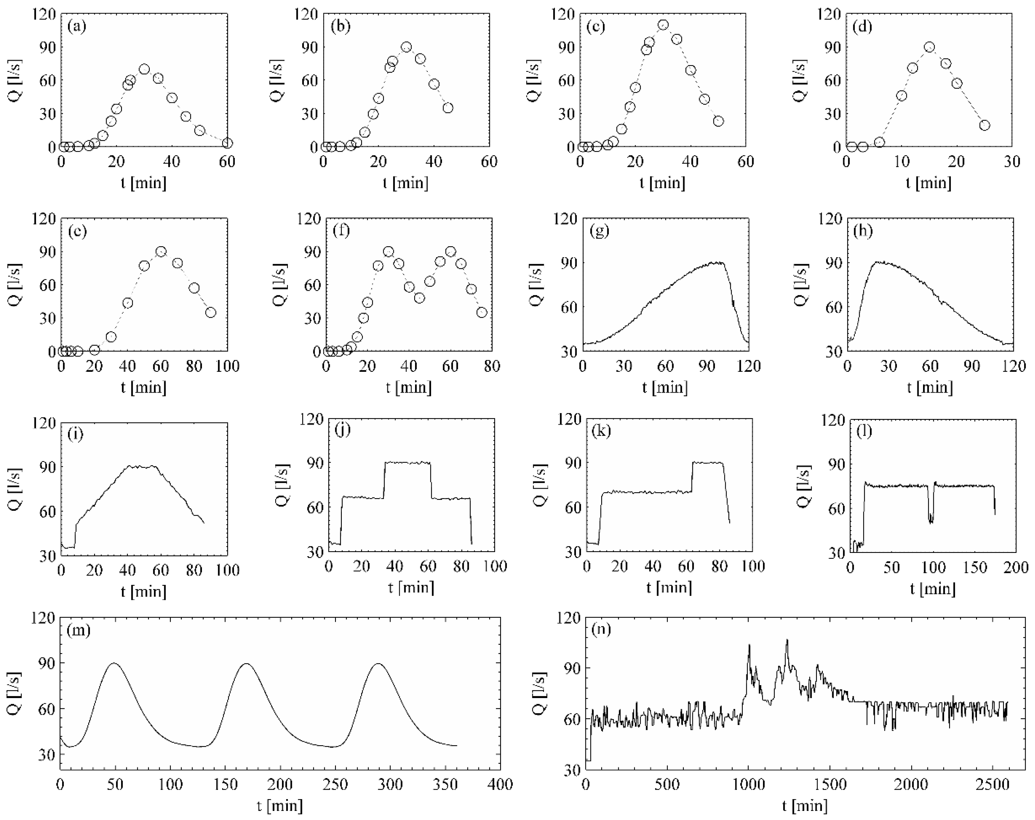
The scour data in Table 1 can be classified as steady or unsteady, depending on the hydraulic conditions in which the experiments were performed. For time-dependent runs, the flow-discharge, flow-velocity, and flow-depth vary in time, whereas the values presented in Table 1 refer to peak flow conditions. Figure 1 shows the hydrographs corresponding to the 14 unsteady runs considered herein. Stepwise hydrographs are presented in Figure 1j–l.
The dataset is composed of natural and artificial sediments as well, with relative densities ranging from 0.04 to 1.65. The ratio between pier-diameter and sediment-size ranges from 11.11 to 4159.09, and the ratio between flow-depth and pier-diameter takes values from 0.12 to 13.20. ranges from 5.06 to 121.42 and thus covered flows with hydraulically smooth, transitional smooth-rough, and rough walls. The considered experimental data refer to clear-water conditions (), allowing the identification of local scour without effects of overlapping processes, such as bedforms migration and scour hole refilling. Only four experiments are catalogued as exceptions to such decisions, in which their flow intensity values are slightly greater than one (2002OLIVETO18S, 2002OLIVETO33S, 1956CHABERT07S, and 1956CHABERT08S). Such exceptions were considered in order to have at least three experiments with the same and different , with the aim of analyzing the sediment and geometrical dependency on (Section 5.2.1).
4.2. , , and Estimation
Sheppard et al. [9] evaluated 23 predictive equilibrium bridge scour depth formulations proposed for simple-shaped structures and founded in cohesionless sediments. The analyzed predictive methods were improved over time in terms of accuracy and the Sheppard/Melville (S/M) formulation was found to be the most accurate for the tested and considered dataset. Consequently, the S/M formulation was taken into account and slightly modified to estimate , , and . Equations (18) to (21) present the original formulation,
in which represents the water depth effect on bridge pier scour, the velocity influence, and denotes scale effects between pier-diameter and sediment-size. Accordingly, and contain the hydraulic impacts on local scour, while denotes scale ratio effects.
Note that the BRISENT model is able to reproduce the scour dynamic until the maximum selected value of . Thus, it is convenient to choose its maximum value, i.e., relating with at equilibrium scour conditions. The laboratory data employed by Sheppard et al. [9] was used in correspondence with their formulation for estimating , , and . Such a dataset consists of 441 laboratory experiments and 791 field data. The original dataset was filtered by three conditions to ensure the calculation of : (1) having complete information about the experiments; (2) clear-water scour; and (3) in order to ensure the scour equilibrium state.
4.3. Calibration and Validation Procedures
All fitting coefficients were determined by MATLAB(MathWorks, Natick, MA, USA) nonlinear curve–fit function, considering and as the last measured point. Therefore, and are not fitting coefficients when the BRISENT model is calibrated with time-dependent scour depth experiments; i.e., experiments that contain the whole scour depth evolution over time. The experiments are presented in Table 1.
Based on the unique relationship between and (under clear-water conditions, constant sediment properties, and geometrical scales) [21], unsteady experiments were calibrated in two ways:
- (a)
- Calibration employing unsteady data: Each unsteady run was calibrated with the aim of finding the best performance of the model. This kind of calibration will be called “unsteady calibration” in the rest of the paper.
- (b)
- Calibration employing steady data: Two steady runs were used to calibrate the model with the aim of testing it in the most critical condition. The values of the dimensionless parameters regarding sediment properties and geometrical scale () are identical for calibration runs as well as for unsteady experiments, respectively. “2002OLIVETO32S” was used to calibrate Oliveto and Hager’s [19] unsteady runs and “2017PIZARRO01S” for the unsteady experiments of Pizarro et al. [21] and Link et al. [22]. This kind of calibration will be called “steady calibration” in the rest of the paper.
Table 2 summarizes calibration results for both calibration types.
The BRISENT model is completely determined when , , and are known. and are estimated employing the S/M formulation and the dataset of Sheppard et al. [9] in order to guarantee equilibrium conditions. This is a critical step for the proper use of the model due to Equation (11).
For validation procedures, the most complex experiments were used among those available to the authors: two highly unsteady and multi-peaked runs pertained to Link et al. [22] (2017LINK01U and 2017LINK02U).
5. Results
5.1. BRISENT as a Multipurpose Model
5.1.1. BRISENT Performance under Steady Hydraulic Conditions
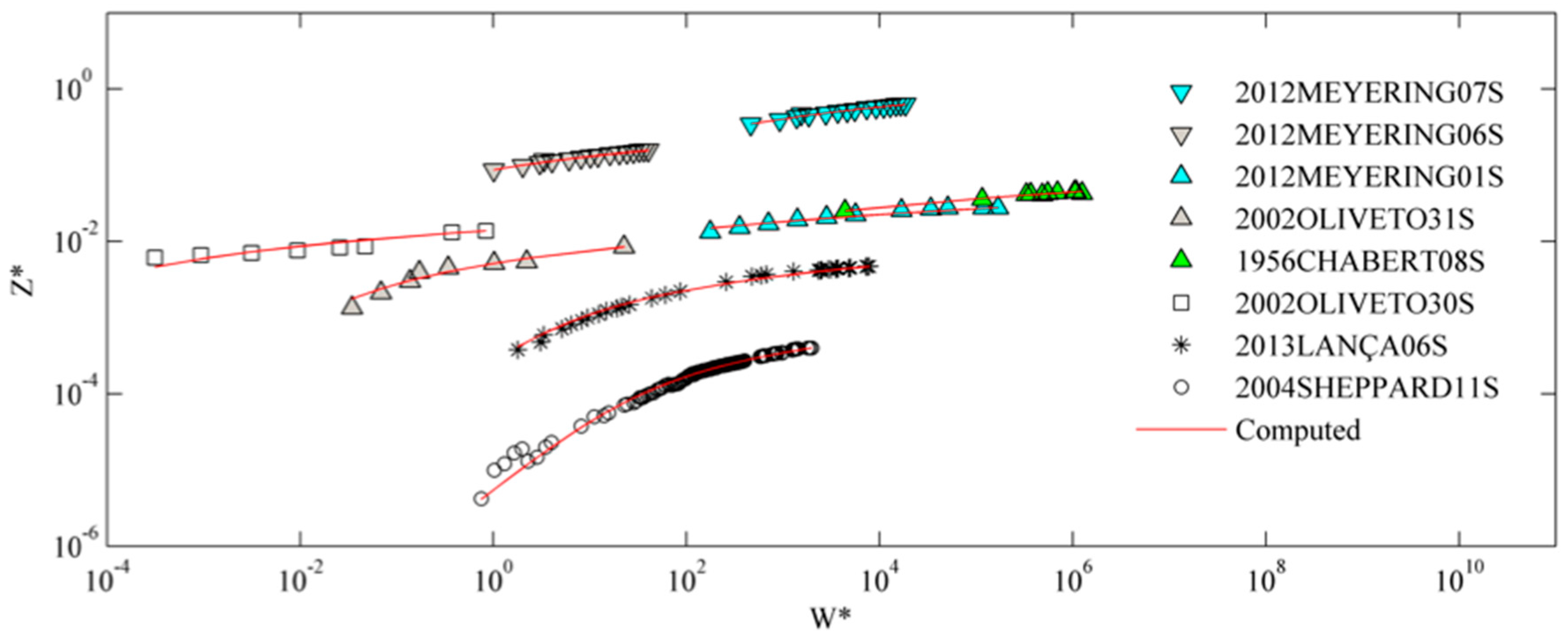
Ninety percent of the experimental data presented in Section 4 were performed under steady hydraulic conditions. Figure 2 illustrates the time-dependent scour depth for different experiments that consider the extreme values of the dimensionless parameters. In all cases, the BRISENT model is able to reproduce the scour evolution with root mean square error (RMSE) values between 0.04 and 1.60 cm. RMSE is defined as ; where is the measured scour depth , is the computed scour depth , and is the number of measured points. Therefore, the proposed BRISENT model can reproduce the scour evolution with high accuracy under steady hydraulic conditions.
Note that the scour evolution presents similar behavior in two groups of experiments (triangle markers). The first group consists of the experiments “2012MEYERING06S” and “2012MEYERING07S”, while the second group consists of the experiments “2012MEYERING01S”, “2002OLIVETO31S”, and “1956CHABERT08S”. Such a similar scour evolution is due to the reduced variability of the dimensionless that takes values around 10 and 120 for the first and second groups, respectively.
5.1.2. BRISENT Performance under Flood Waves
Figure 3 presents the time-dependent evolution of the measured scour depth in contrast to the BRISENT model calibrated according to the procedure presented in Section 4.3. Table 3 summarizes the model benchmarking in terms of RMSE for each experiment. The results show that, independently of the kind of calibration, BRISENT correctly reproduces the time-dependent scour depth with RMSE values less than 1.57 and 0.52 cm for steady and unsteady calibrations, respectively.
Steady calibration tends to overestimate the maximum scour depths after flood waves, while unstedy calibration presents better performances in all analyzed experiments. Furthermore, the average RMSE values are less than 1 cm, independetly of the kind of calibration. Therefore, the proposed BRISENT model can reproduce the scour evolution with high accuracy under stepwise hydrographs and 100% unsteady hydraulic conditions.
5.2. In Search of a Practical Formulation
5.2.1. Effects of and on
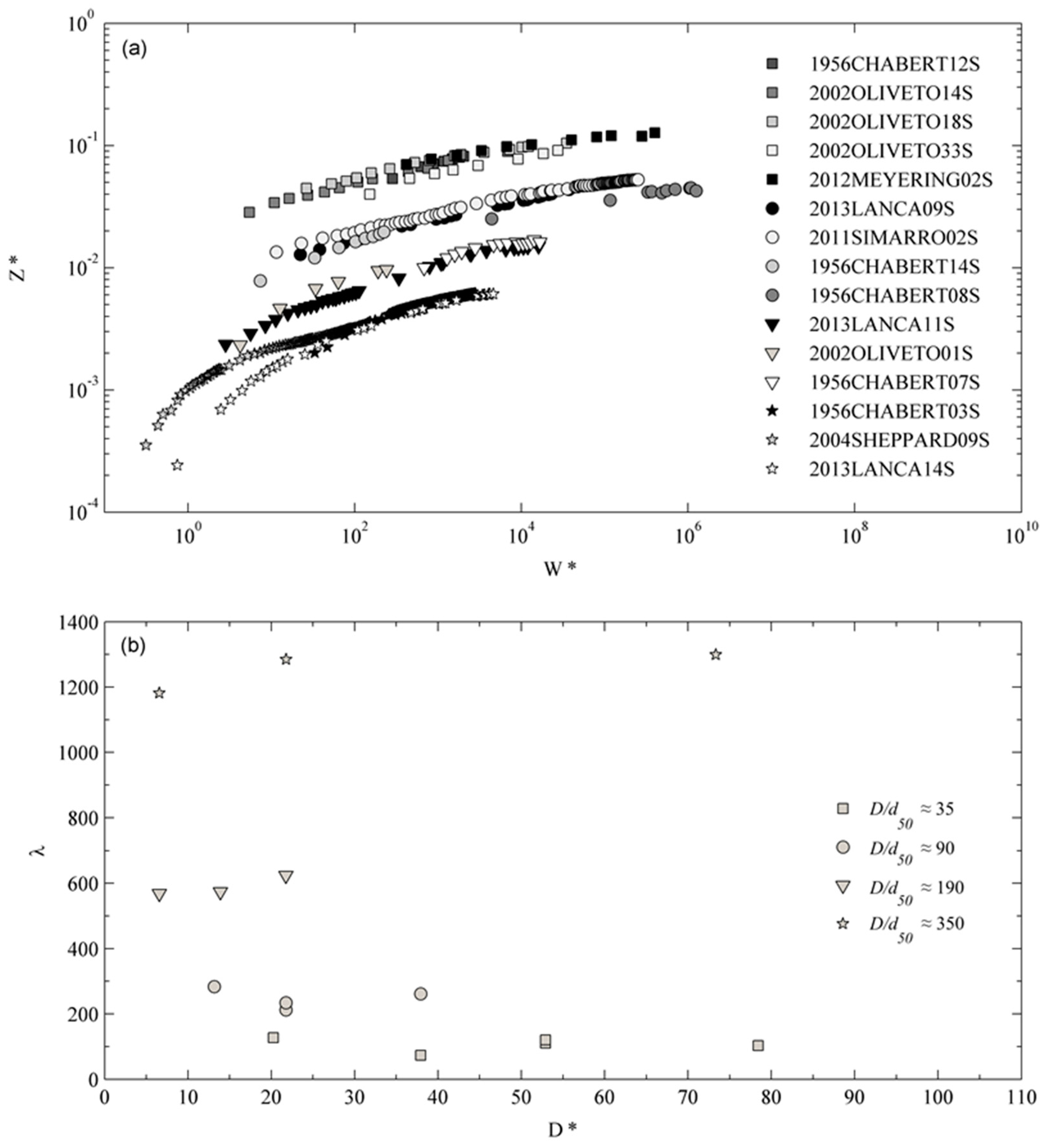
A selected group of 15 experimental runs was considered to analyze the sediment and geometrical dependency on . This number was established in order to have at least three experiments with the same and different . The data were categorized in four classes depending on the geometrical scale between pier-diameter and sediment-size (35, 90, 190, and 350). The range for the dimensionless particle diameter takes values from 6.58 to 78.42. Figure 4a shows the evolution of over according to the four classes. All data collapse into a single and geometrically-dependent curve, independently of the hydraulic conditions. Z* decreases with for equal .
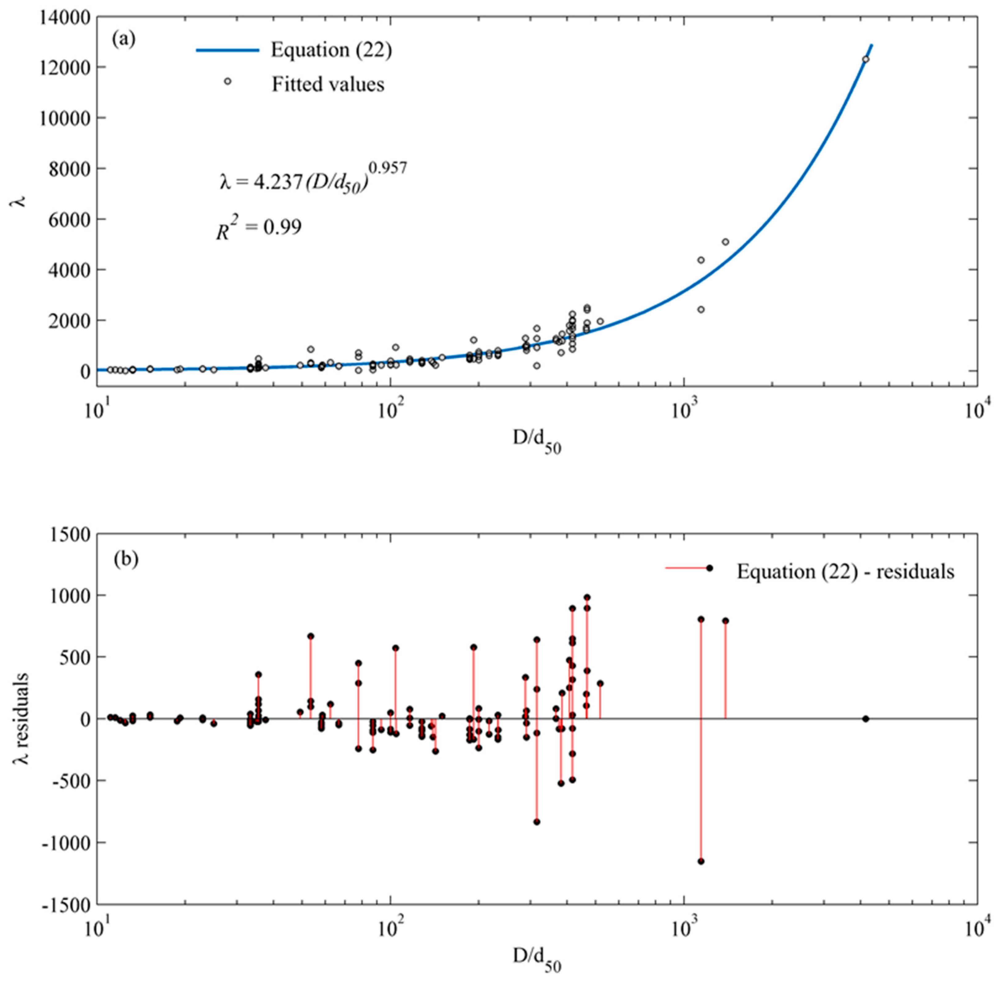
Figure 4b shows calibrated on . No correlation between these two variables is detected and it can be observed that is strongly controlled by . A power function is adopted in order to describe this dependency:
where and are fitting coefficients that were determined by the procedure presented in Section 4.3, obtaining and with a determination coefficient and a RMSE equal to 49. Equation (22) is plotted in Figure 5a in comparison to the fitted values and Figure 5b presents the residuals between calibrated and estimated .
The fitting coefficient is always affected by the ratio between pier-diameter and sediment size, even for high values. Thus, a stabilizer or equilibrium threshold for it was not found.
5.2.2. , , and Estimation
As mentioned in Section 4.2, the S/M formulation was taken into consideration and Equation (18) can be multiplied by in order to have on the left side of the equation,
The hydraulic effects in the original S/M formulation are represented by and . On the other hand, has the capacity to integrate these hydraulic effects on the local scour process. Therefore, and can take a convenient value with the aim of writing it in a function of . Considering makes it possible to be on the safe side from a design perspective and, consequently, this value was selected:
From the experimental data of Sheppard et al. [9], only 129 of the total experiments were considered after applying the filters described in Section 4.3. Table 4 summarizes the source for laboratory data, the number of experiments from the source, and the range of selected dimensionless parameters according to the filtered dataset.
versus values are plotted in Figure 6, in which the solid line represents Equation (25):
where and are fitting coefficients that were calibrated by the procedure described in Section 4.3, obtaining and with a determination coefficient and a RMSE = 1.19.
Therefore, can be evaluated by Equation (26) and the entropic scour parameter S can be estimated with Equation (27) (Equation (13) in combination with Equation (24)):
5.3. BRISENT Validation: Highly Unsteady and Multi-Peaked Hydrographs
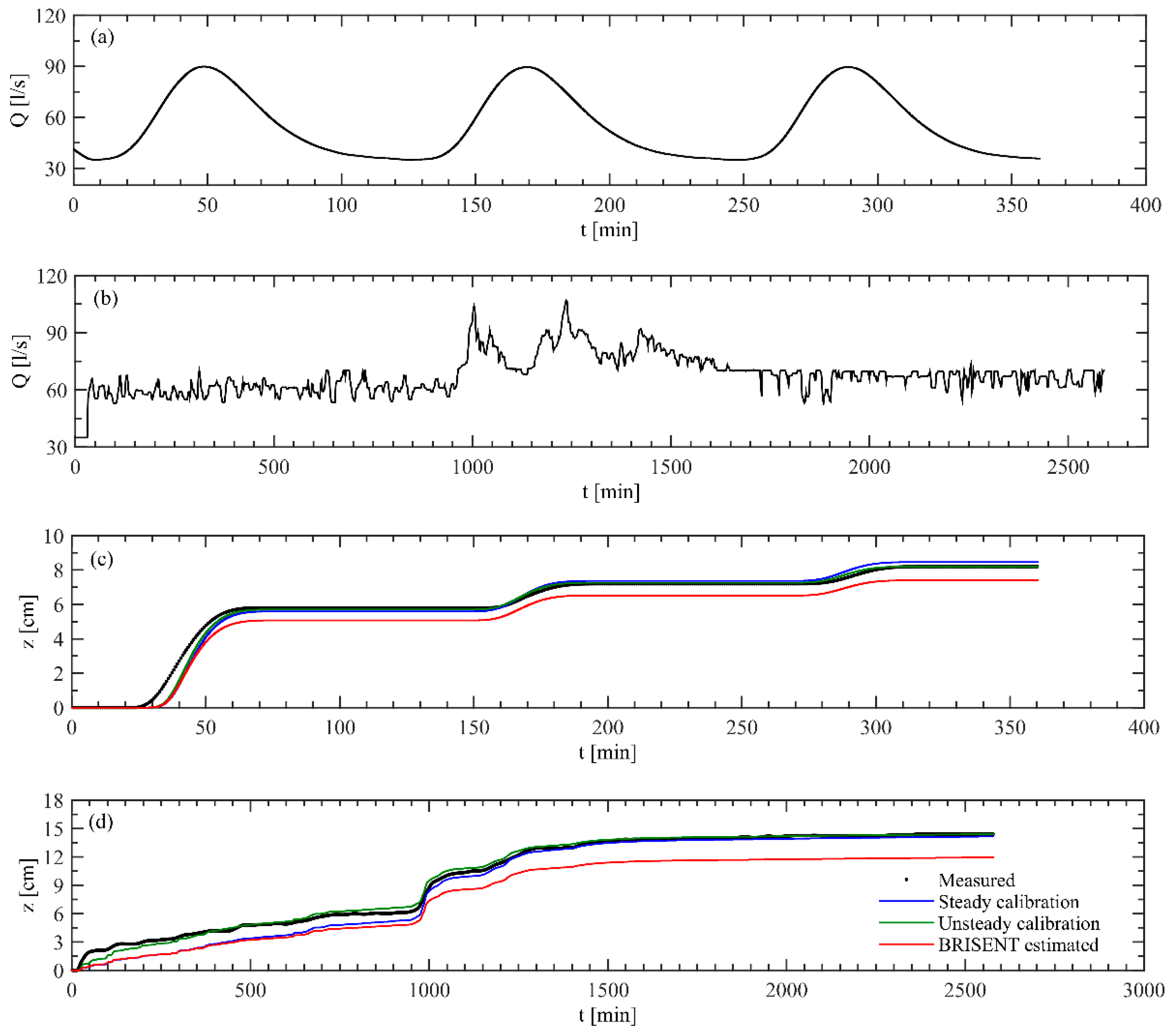
The BRISENT model was validated using highly unsteady and multi-peaked hydrographs pertaining to Link et al. [22]. Validation runs are plotted on Figure 7a–d, presenting the time-dependent evolution of the measured scour depth in contrast to the BRISENT model calibrated and estimated according to the proposed equations (Equations (22), (26) and (27)).
Table 5 summarizes the model benchmarking in terms of RMSE for experiments “2017LINK01U” and “2017LINK02U”, and the results show that the proposed equations correctly reproduce the main dynamic of the time-dependent scour depth. Note that the unsteady calibration provides the most accurate results with RMSE values less than 0.32 cm, while the observed higher RMSE values for the estimated BRISENT model rely on the computed values of . Steady calibration shows good performance as well, with RMSE values less than 0.81 cm.
6. Discussion
6.1. Informational Entropy and the Principle of Maximum Entropy for Pier Scour Modelling
From a practical perspective, traditional bridge scour formulas are used in order to estimate a potential scour depth that could occur during bridge life. However, neither a vectorial nor a empirical approach can estimate the scour process by considering long duration events, discharge regime, and the interactions of different erosional processes. Therefore, scour depth estimations are uncertain.
The informational entropy concept has long been recognized as a measure of uncertainties, and is the ideal concept for analyzing the bridge scour phenomenon. Moreover, BRISENT is based on the effective flow work parameter and thus, the combination of and the principle of maximum entropy (POME) is a variational/thermodynamic approach for treating the scour process. The fact that the core of the model is based on the informational entropy concept (uncertainty) presents a clear advantage in comparison to other formulations by taking into consideration bridge design, bridge life, and hydrologic regime.
6.2. BRISENT: A Multipurpose Model
BRISENT was inferred without imposing the hydraulic conditions, under which the model can run. In particular, the results confirm that the BRISENT model can be used under different and complex hydraulic conditions (steady flows, step-wise hydrographs, and flood waves with multi-peaked hydrographs) to describe bridge scour phenomena, and independently of the type of calibration. In consequence, BRISENT can be considered a multipurpose model which allows calibration under simple hydraulic conditions and application to more complex and realistic hydraulic situations. Since, in the past, most scour experiments were carried out under steady hydraulic conditions, these are clear advantages over other published formulations.
6.3. Wide Range of the Considered Dimensionless Parameters
Two hundred and sixty-six clear-water scour experiments were considered for the calibration process, with widely ranging dimensionless parameters. For example, ranges from 5.06 to 121.42 and, thus, covered flows with hydraulically smooth, transitional smooth–rough, and rough walls, according to Oliveto and Hager [66]. The ratio between pier-diameter and sediment-size ranges from 11.11 to 4159.09 and, thus, the obtained results can be used in both laboratory and natural scales. The same can be said for the ratio between flow-depth and pier-diameter, which takes values from 0.12 to 13.20.
6.4. Applicability of the Model: Advantages and Limitations
Simple equations are proposed to estimate the time-dependent scour depth independently of hydraulic conditions, geometrical scale, and hydraulic flow roughness. Equation (26) and Equation (27) are empiric equations for and which are based on the dataset published by Sheppard et al. [9]. Such dataset contains a wide value range of dimensionless parameters, making it possible to treat the bridge scour phenomenon under different flow regimes and different geometrical scales. Furthermore, the results show that the proposed equations correctly reproduce the main dynamic of the time-dependent scour depth under clear-water conditions, where no overlapping of other erosional processes occur.
6.5. Key Dimensionless Parameters: and
The ratio between pier-diameter and sediment-size (geometrical scale) is the most critical physical characteristic controlling the scour model parametrization. From a physical modeling perspective, keeping constant a high value of at laboratory scales is very hard due to the sediment cohesion (sediment size has to be reduced 10 times or more in laboratory flumes). As a consequence, theoretical efforts to develop new and more accurate models are a major challenge in this field, where the BRISENT model represents the first model of its kind. Additionally, our results highlight that the key dimensionless parameters are and . Such parameters contain the energy for undermining and the geometrical scale between pier diameter and sediment size, respectively. More energy to reach the same relative scour depth at a real scale was observed, thus positioning laboratory-deduced formulas on the side of safety from a design perspective.
7. Conclusions
Bridge-pier scour evolution has been analyzed in the present work, using the first mathematical formulation for simulating scour phenomena based on energy concepts and entropy theory. The proposed BRISENT model has been established on the effective flow work parameter ) and on the principle of maximum entropy (POME). The results confirm the idea that the local-scour phenomenon indirectly depends on the time-dependent mean velocity, and thus the model can be calibrated using steady scour data and applied to more complex hydraulic scenarios. Literature data under clear-water conditions were employed, in which the key dimensionless parameters took values over a wide range, allowing analysis of the local scour phenomenon from a holistic point of view. Simple formulations were proposed to estimate the fitting coefficient (Equation (22)) and the entropic-scour parameter (Equation (27)). Moreover, we observed that the ratio is the most critical physical characteristic controlling the scour model parametrization.
Our results support the idea that POME and could be used to explain erosional processes and, in particular, to describe clear-water local-scour phenomena with high accuracy and simple formulations. This is an entry point for treating more complex river interaction processes at different spatial scales (e.g., channel instability, channel bed gradation, channel migration, contraction scour, local scour, etc.). The authors are keen to apply these concepts with the aim of answering the following questions: (i) how long does it take to reach the equilibrium state under clear-water, bed-load, suspension conditions and/or a possible combination of scour modes at real piers? (ii) is it achievable during the lifetime of bridges? (iii) how does the scour-hole refilling process affect the whole scour dynamic? (iv) what is the time-evolution of and ?
Acknowledgments
The authors would like to thank Professor Giuseppe Oliveto (University of Basilicata) for providing his experimental data, and the support of the European Commission under the ELARCH program (Project Reference number: 552129-EM-1-2014-1-IT-ERA MUNDUS-EMA21). OL thanks the Chilean Research Council CONICYT for the research project FONDECYT 1150997 “Bridge pier scour under flood waves”. This publication reflects the authors’ view only and the Commission is not liable for any use that may be made of the information contained therein. The constructive comments of four anonymous reviewers are gratefully appreciated and the review comments helped to substantially improve the paper. This work was carried out within the scientific agreement between the Civil Protection of Basilicata, the CINID and the University of Basilicata for the startup of the Functional Center of Basilicata.
Author Contributions
All authors made a substantial contribution to this paper. A.P. conceived the model, wrote the first draft, and submitted the manuscript. M.F. added entropic ideas to the study. C.S. contributed to the data analysis and improvement of the document. O.L. and S.M. designed and mentored the research and contributed to the results interpretation.
Conflicts of Interest
The authors declare no conflict of interest.
References
- Briaud, J.L.; Brandimarte, L.; Wang, J.; D’Odorico, P. Probability of scour depth exceedance owing to hydrologic uncertainty. Georisk Assess. Manag. Risk Eng. Syst. Geohazards 2007, 1, 77–88. [Google Scholar] [CrossRef]
- Cook, W. Bridge Failure Rates, Consequences, and Predictive Trends; Utah State University: Logan, UT, USA, 2014; ISBN 1321576021. [Google Scholar]
- Imam, B.M.; Marios, K. Causes and consequences of metallic bridge failures. Struct. Eng. Int. 2012, 22, 93–98. [Google Scholar] [CrossRef]
- Kattell, J.; Eriksson, M. Bridge Scour Evaluation: Screening, Analysis, & Countermeasures; San Dimas Technology and Development Center: San Dimas, CA, USA, 1998. [Google Scholar]
- Smith, D.W. Bridge failures. Proc. Inst. Civ. Eng. 1976, 60, 367–382. [Google Scholar] [CrossRef]
- Wardhana, K.; Hadipriono, F.C. Analysis of recent bridge failures in the United States. J. Perform. Constr. Facil. 2003, 17, 144–150. [Google Scholar] [CrossRef]
- Melville, B.W. Pier and abutment scour: Integrated approach. J. Hydraul. Eng. 1997, 123, 125–136. [Google Scholar] [CrossRef]
- Richardson, E.V.; Davis, S.R. Evaluating Scour at Bridges: Hydraulic Engineering Circular No. 18; Federal Highway Administration: Washington, DC, USA, 1995. [Google Scholar]
- Sheppard, D.M.; Melville, B.; Demir, H. Evaluation of Existing Equations for Local Scour at Bridge Piers. J. Hydraul. Eng. 2014, 140, 14–23. [Google Scholar] [CrossRef]
- Zanke, U. Kolke am Pfeiler in richtungskonstanter Strömung und unter Welleneinfluß; Universität Hannover: Hannover, Germany, 1982; Volume 54, pp. 381–416. [Google Scholar]
- Manes, C.; Brocchini, M. Local scour around structures and the phenomenology of turbulence. J. Fluid Mech. 2015, 779, 309–324. [Google Scholar] [CrossRef]
- Dey, S. Time-variation of scour in the vicinity of circular piers. Proc. Inst. Civ. Eng. Marit. Energy 1999, 136, 67–75. [Google Scholar] [CrossRef]
- Melville, B.W.; Chiew, Y.-M. Time scale for local scour at bridge piers. J. Hydraul. Eng. 1999, 125, 59–65. [Google Scholar] [CrossRef]
- Oliveto, G.; Hager, W.H. Temporal evolution of clear-water pier and abutment scour. J. Hydraul. Eng. 2002, 128, 811–820. [Google Scholar] [CrossRef]
- Sheppard, D.M.; Miller, W., Jr. Live-bed local pier scour experiments. J. Hydraul. Eng. 2006, 132, 635–642. [Google Scholar] [CrossRef]
- Lai, J.-S.; Chang, W.-Y.; Yen, C.-L. Maximum local scour depth at bridge piers under unsteady flow. J. Hydraul. Eng. 2009, 135, 609–614. [Google Scholar] [CrossRef]
- Kothyari, U.C.; Garde, R.C.J.; Ranga Raju, K.G. Temporal variation of scour around circular bridge piers. J. Hydraul. Eng. 1992, 118, 1091–1106. [Google Scholar] [CrossRef]
- López, G.; Teixeira, L.; Ortega-Sánchez, M.; Simarro, G. Estimating final scour depth under clear-water flood waves. J. Hydraul. Eng. 2014, 140, 328–332. [Google Scholar] [CrossRef]
- Oliveto, G.; Hager, W.H. Further results to time-dependent local scour at bridge elements. J. Hydraul. Eng. 2005, 131, 97–105. [Google Scholar] [CrossRef]
- Hager, W.H.; Unger, J. Bridge pier scour under flood waves. J. Hydraul. Eng. 2010, 136, 842–847. [Google Scholar] [CrossRef]
- Pizarro, A.; Ettmer, B.; Manfreda, S.; Rojas, A.; Link, O. Dimensionless effective flow work for estimation of pier scour caused by flood waves. J. Hydraul. Eng. 2017, 143. [Google Scholar] [CrossRef]
- Link, O.; Castillo, C.; Pizarro, A.; Rojas, A.; Ettmer, B.; Escauriaza, C.; Manfreda, S. A model of bridge pier scour during flood waves. J. Hydraul. Res. 2017, 55. [Google Scholar] [CrossRef]
- Sturm, T.; Sotiropoulos, F.; Landers, M.; Gotvald, T.; Lee, S.; Ge, L.; Navarro, R.; Escauriaza, C. Laboratory and 3D numerical modeling with field monitoring of regional bridge scour in Georgia. In Georgia Department of Transportation Final Project; Georgia Dept. of Transportation: Atlanta, GA, USA, 2004. [Google Scholar]
- Clubley, S.K.; Manes, C.; Richards, D.J. High resolution sonars set to revolutionise bridge scour inspections. Proc. Inst. Civ. Eng. Civ. Eng. 2015, 168, 35–42. [Google Scholar] [CrossRef]
- Prendergast, L.J.; Gavin, K. A review of bridge scour monitoring techniques. J. Rock Mech. Geotech. Eng. 2014, 6, 138–149. [Google Scholar] [CrossRef]
- Hong, J.-H.; Guo, W.-D.; Chiew, Y.-M.; Chen, C.-H. A new practical method to simulate flood-induced bridge pier scour—A case study of Mingchu bridge piers on the Cho-Shui River. Water 2016, 8, 238. [Google Scholar] [CrossRef]
- Su, C.-C.; Lu, J.-Y. Comparison of Sediment Load and Riverbed Scour during Floods for Gravel-Bed and Sand-Bed Reaches of Intermittent Rivers: Case Study. J. Hydraul. Eng. 2016, 142, 5016001. [Google Scholar] [CrossRef]
- Gaudio, R.; Grimaldi, C.; Tafarojnoruz, A.; Calomino, F. Comparison of formulae for the prediction of scour depth at piers. In Proceedings of the 1st IAHR European Division Congress, Edinburgh, UK, 4–6 May 2010. [Google Scholar]
- Gaudio, R.; Tafarojnoruz, A.; De Bartolo, S. Sensitivity analysis of bridge pier scour depth predictive formulae. J. Hydroinform. 2013, 15, 939–951. [Google Scholar] [CrossRef]
- Barbe, D.E.; Cruise, J.F.; Singh, V.P. Probabilistic approach to local bridge pier scour. Transp. Res. Rec. 1350 1992, 28–33. Available online: https://trid.trb.org/view.aspx?id=370731 (accessed on 5 November 2017).
- Johnson, P.A. Reliability-based pier scour engineering. J. Hydraul. Eng. 1992, 118, 1344–1358. [Google Scholar] [CrossRef]
- Johnson, P.A. Fault tree analysis of bridge failure due to scour and channel instability. J. Infrastruct. Syst. 1999, 5, 35–41. [Google Scholar] [CrossRef]
- Johnson, P.A.; Ayyub, B.M. Assessing time-variant bridge reliability due to pier scour. J. Hydraul. Eng. 1992, 118, 887–903. [Google Scholar] [CrossRef]
- Johnson, P.A.; Ayyub, B.M. Modeling uncertainty in prediction of pier scour. J. Hydraul. Eng. 1996, 122, 66–72. [Google Scholar] [CrossRef]
- Johnson, P.A.; Hell, T.M. Bridge Scour-A Probabilistic Approach. Infrastruct. Sussex 1996, 1, 24–30. [Google Scholar]
- Johnson, P.A.; Dock, D.A. Probabilistic bridge scour estimates. J. Hydraul. Eng. 1998, 124, 750–754. [Google Scholar] [CrossRef]
- Yanmaz, A.M.; Cicekdag, O. Composite reliability model for local scour around cylindrical bridge piers. Can. J. Civ. Eng. 2001, 28, 520–535. [Google Scholar] [CrossRef]
- Yanmaz, A.M.; Üstün, I. Generalized reliability model for local scour around bridge piers of various shapes. Turk. J. Eng. Environ. Sci. 2001, 25, 687–698. [Google Scholar]
- Johnson, P.A.; Clopper, P.E.; Zevenbergen, L.W.; Lagasse, P.F. Quantifying uncertainty and reliability in bridge scour estimations. J. Hydraul. Eng. 2015, 141, 4015013. [Google Scholar] [CrossRef]
- Flint, M.M.; Fringer, O.; Billington, S.L.; Freyberg, D.; Diffenbaugh, N.S. Historical Analysis of Hydraulic Bridge Collapses in the Continental United States. J. Infrastruct. Syst. 2017, 23, 4017005. [Google Scholar] [CrossRef]
- Robinson, D.W. Entropy and uncertainty. Entropy 2008, 10, 493–506. [Google Scholar] [CrossRef]
- Wang, Q.A. Probability distribution and entropy as a measure of uncertainty. J. Phys. A Math. Theor. 2008, 41, 65004. [Google Scholar] [CrossRef]
- Koutsoyiannis, D. Entropy: From thermodynamics to hydrology. Entropy 2014, 16, 1287–1314. [Google Scholar] [CrossRef]
- Dong, X.; Lu, H.; Xia, Y.; Xiong, Z. Decision-Making Model under Risk Assessment Based on Entropy. Entropy 2016, 18, 404. [Google Scholar] [CrossRef]
- Kvålseth, T.O. On the measurement of randomness (uncertainty): A more informative entropy. Entropy 2016, 18, 159. [Google Scholar] [CrossRef]
- Jaynes, E.T. Information theory and statistical mechanics. II. Phys. Rev. 1957, 108, 171. [Google Scholar] [CrossRef]
- Chiu, C.-L. Entropy and probability concepts in hydraulics. J. Hydraul. Eng. 1987, 113, 583–599. [Google Scholar] [CrossRef]
- Fiorentino, M.; Claps, P.; Singh, V.P. An entropy-based morphological analysis of river basin networks. Water Resour. Res. 1993, 29, 1215–1224. [Google Scholar] [CrossRef]
- Singh, V.P. Entropy theory for movement of moisture in soils. Water Resour. Res. 2010, 46, W0516. [Google Scholar] [CrossRef]
- Singh, V.P. Entropy theory for derivation of infiltration equations. Water Resour. Res. 2010, 46, W03527. [Google Scholar] [CrossRef]
- Singh, V.P. Entropy Theory in Hydraulic Engineering: An Introduction; American Society of Civil Engineers: Reston, VA, USA, 2014. [Google Scholar] [CrossRef]
- Singh, V.P. Entropy Theory in Hydrologic Science and Engineering; McGraw Hill Professional: New York, NY, USA, 2014; ISBN 0071835474. [Google Scholar]
- Moramarco, T.; Corato, G.; Melone, F.; Singh, V.P. An entropy-based method for determining the flow depth distribution in natural channels. J. Hydrol. 2013, 497, 176–188. [Google Scholar] [CrossRef]
- Hemelrijk, J. Underlining random variables. Stat. Neerl. 1966, 20, 1–7. [Google Scholar] [CrossRef]
- Breusers, H.N.C.; Nicollet, G.; Shen, H.W. Local scour around cylindrical piers. J. Hydraul. Res. 1977, 15, 211–252. [Google Scholar] [CrossRef]
- May, R.W.P.; Willoughby, I.R. Local Scour around Large Obstructions; Technical Report; Hydraulics Research: Wallingford, Oxfordshire, UK, 1990. [Google Scholar]
- Miller, W., Jr.; Sheppard, D.M. Time rate of local scour at a circular pile. In Proceedings of the First International Conference on Scour of Foundations, College Station, TX, USA, 17–20 November 2002. [Google Scholar]
- Chabert, J.; Engeldinger, P. Etude des Affouillements Autour des Piles des Ponts; Laboratoire National d’Hydraulique: Chatou, France, 1956; p. 118. (In French) [Google Scholar]
- Franzetti, S.; Larcan, E.; Mignosa, P. Erosione alla base di pile circolari di ponte: Verifica sperimentale dell’ipotesi di esistenza di una situazione finale di equilibrio. Idrotecnica 1989, 16, 135–141. [Google Scholar]
- Sheppard, D.M.; Odeh, M.; Glasser, T. Large scale clear-water local pier scour experiments. J. Hydraul. Eng. 2004, 130, 957–963. [Google Scholar] [CrossRef]
- Grimaldi, C. Non-Conventional Countermeasures Against Local Scouring at Bridge Piers. Ph.D. Thesis, The Hydraulic Engineering for Environment and Territory University, Cosenza, Italy, 2005. [Google Scholar]
- Alabi, P.D. Time Development of Local Scour at a Bridge Pier Fitted with a Collar. Master’s Thesis, University of Saskatchewan, Saskatoon, SK, Canada, 2006. [Google Scholar]
- Simarro, G.; Fael, C.M.S.; Cardoso, A.H. Estimating equilibrium scour depth at cylindrical piers in experimental studies. J. Hydraul. Eng. 2011, 137, 1089–1093. [Google Scholar] [CrossRef]
- Meyering, H. Effect of Sediment Density in Bridge Pier Scour Experiments. Ph.D. Thesis, Technical University of Braunschweig, Braunschweig, Germany, 2012. [Google Scholar]
- Lança, R.M.; Fael, C.S.; Maia, R.J.; Pêgo, J.P.; Cardoso, A.H. Clear-water scour at comparatively large cylindrical piers. J. Hydraul. Eng. 2013, 139, 1117–1125. [Google Scholar] [CrossRef]
- Giuseppe, O.; Hager, H.W. Closure to “Further Results to Time-Dependent Local Scour at Bridge Elements” by Giuseppe Oliveto and Willi H. Hager. J. Hydraul. Eng. 2006, 132, 997–998. [Google Scholar] [CrossRef]
Figure 1.
Unsteady runs employed in this study. Images (a–f) are experiments 2005OLIVETO01U, 2005OLIVETO02U, 2005OLIVETO03U, 2005OLIVETO04U, 2005OLIVETO05U and 2005OLIVETO06U, respectively; images (g–l) are experiments 2017PIZARRO01U, 2017PIZARRO02U, 2017PIZARRO03U, 2017PIZARRO04U, 2017PIZARRO05U and 2017PIZARRO06U, respectively; and images (m,n) are experiments 2017LINK01U and 2017LINK02U, respectively.

Figure 2.
Measured (markers) and computed scour depth evolution using BRISENT model (red line) for experiments with extreme values of , , , , and .
Figure 2.
Measured (markers) and computed scour depth evolution using BRISENT model (red line) for experiments with extreme values of , , , , and .

Figure 3.
Benchmarking of the BRISENT model with calibrated with steady and unsteady runs. Images (a–f) are experiments 2005OLIVETO01U, 2005OLIVETO02U, 2005OLIVETO03U, 2005OLIVETO04U, 2005OLIVETO05U and 2005OLIVETO06U, respectively; images (g–l) are experiments 2017PIZARRO01U, 2017PIZARRO02U, 2017PIZARRO03U, 2017PIZARRO04U, 2017PIZARRO05U and 2017PIZARRO06U, respectively.
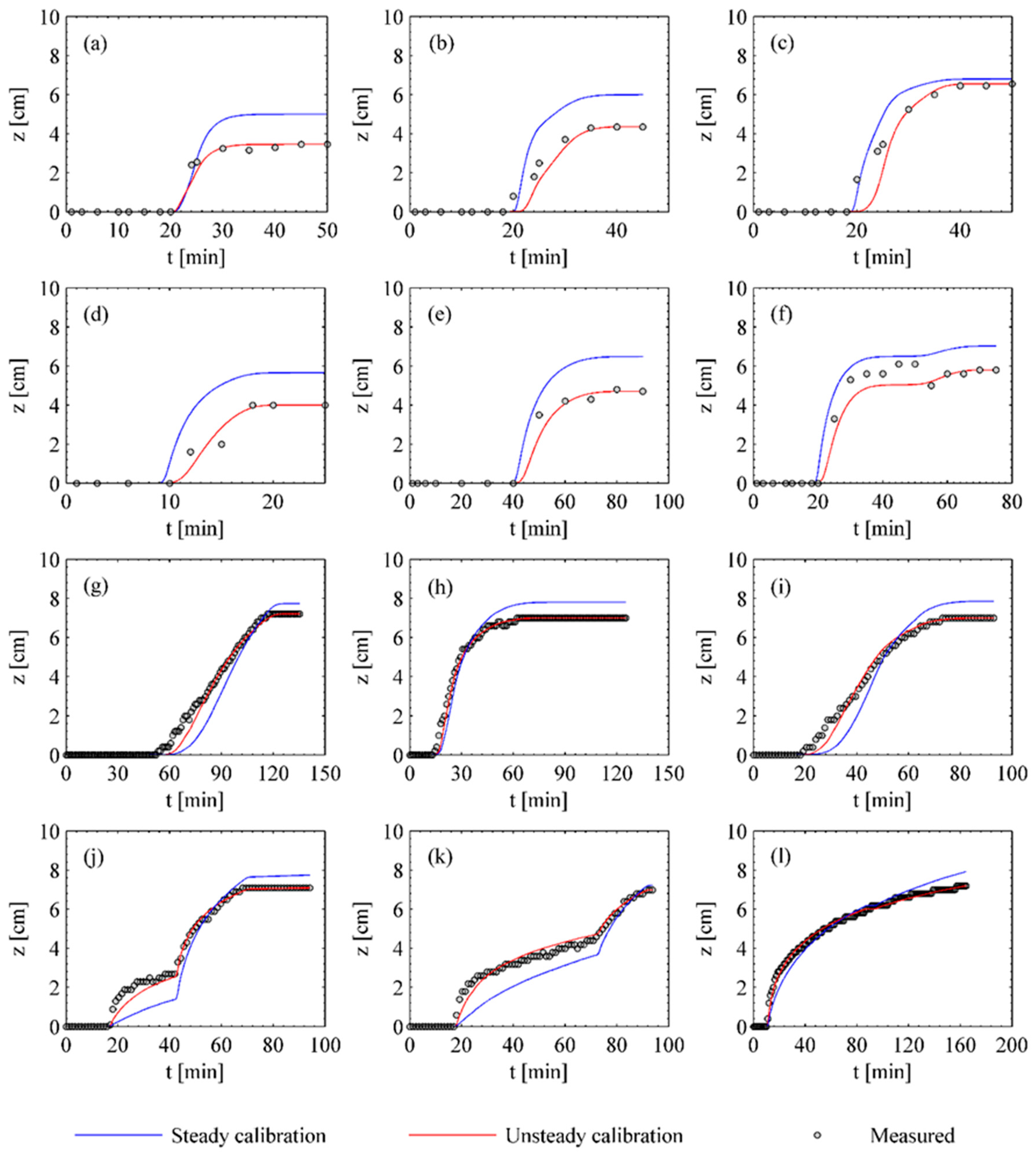
Figure 4.
(a) Relative scour evolution over W* for the four categorized classes; (b) λ calibrated values in function of the dimensionless particle diameter D*.
Figure 4.
(a) Relative scour evolution over W* for the four categorized classes; (b) λ calibrated values in function of the dimensionless particle diameter D*.

Figure 5.
(a) values in function of ; (b) Residual values for in comparison with estimated values using Equation (18).
Figure 5.
(a) values in function of ; (b) Residual values for in comparison with estimated values using Equation (18).

Figure 6.
versus values for the filtered dataset in comparison with the fitting function Equation (25). Data source: Sheppard et al. [9].
Figure 6.
versus values for the filtered dataset in comparison with the fitting function Equation (25). Data source: Sheppard et al. [9].
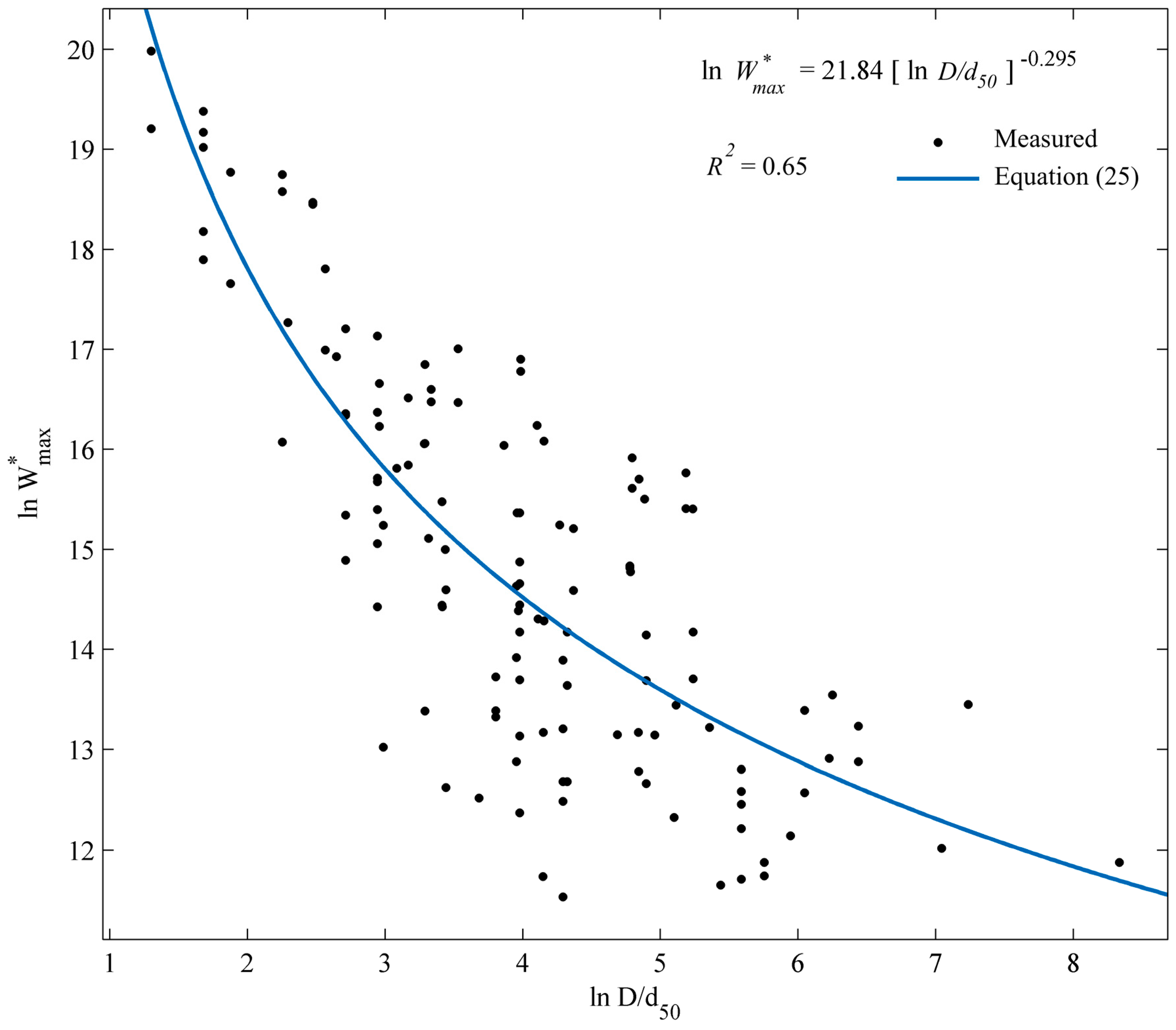
Figure 7.
Validation of the BRISENT model with highly unsteady experiments. Images (a,b) are experiments 2017LINK01U and 2017LINK02U, respectively. Images (c,d) present measured scour depths over time, BRISENT model calibrated using a steady run, BRISENT model calibrated using unsteady runs, and BRISENT model considering Equation (13) to Equation (14) and Equation (19) to Equation (22) for experiments 2017LINK01U and 2017LINK02U, respectively.

Table 1.
Characterization of the experimental data employed for λ estimation.
| Authors | Run | (Days) | ||||||
|---|---|---|---|---|---|---|---|---|
| Chabert and Engeldinger [58] | 1956CHABERT01S | 0.26 | 4.29 | 6.58 | 1.65 | 192.26 | 4.00 | 0.75 |
| 1956CHABERT02S | 0.26 | 4.29 | 6.58 | 1.65 | 288.46 | 2.67 | 0.75 | |
| 1956CHABERT03S | 0.26 | 4.29 | 6.58 | 1.65 | 384.62 | 2.00 | 0.75 | |
| 1956CHABERT04S | 0.26 | 3.92 | 6.58 | 1.65 | 192.26 | 7.00 | 0.92 | |
| 1956CHABERT05S | 0.26 | 3.92 | 6.58 | 1.65 | 288.46 | 4.67 | 0.92 | |
| 1956CHABERT06S | 0.26 | 3.92 | 6.58 | 1.65 | 384.62 | 3.50 | 0.92 | |
| 1956CHABERT07S | 0.26 | 0.55 | 6.58 | 1.65 | 192.26 | 2.00 | 1.20 | |
| 1956CHABERT08S | 0.52 | 6.75 | 13.15 | 1.65 | 96.13 | 2.00 | 1.52 | |
| 1956CHABERT09S | 1.50 | 5.29 | 37.94 | 1.65 | 33.32 | 2.00 | 0.97 | |
| 1956CHABERT10S | 1.50 | 5.29 | 37.94 | 1.65 | 66.67 | 1.00 | 0.97 | |
| 1956CHABERT11S | 1.50 | 5.29 | 37.94 | 1.65 | 100.00 | 0.67 | 0.97 | |
| 1956CHABERT12S | 1.50 | 1.68 | 37.94 | 1.65 | 33.32 | 4.00 | 0.69 | |
| 1956CHABERT13S | 1.50 | 1.68 | 37.94 | 1.65 | 66.67 | 2.00 | 0.69 | |
| 1956CHABERT14S | 1.50 | 1.68 | 37.94 | 1.65 | 100.00 | 1.33 | 0.69 | |
| 1956CHABERT15S | 1.50 | 7.29 | 37.94 | 1.65 | 33.32 | 7.00 | 0.74 | |
| 1956CHABERT16S | 1.50 | 7.29 | 37.94 | 1.65 | 66.67 | 3.50 | 0.74 | |
| 1956CHABERT17S | 1.50 | 7.29 | 37.94 | 1.65 | 100.00 | 2.33 | 0.74 | |
| Zanke [10] | 1982ZANKE01S | 0.24 | 0.002 | 5.84 | 1.65 | 375.00 | 4.67 | 0.75 |
| Franzetti et al. [59] | 1989FRANZETTI01S | 2.50 | 58.13 | 30.22 | 0.18 | 19.20 | 3.00 | 0.79 |
| Oliveto and Hager [14,19] | 2002OLIVETO01S | 0.55 | 0.04 | 13.91 | 1.65 | 200.00 | 1.40 | 0.96 |
| 2002OLIVETO02S | 0.55 | 0.93 | 13.91 | 1.65 | 200.00 | 1.35 | 0.70 | |
| 2002OLIVETO03S | 0.55 | 0.44 | 13.91 | 1.65 | 200.00 | 2.75 | 0.66 | |
| 2002OLIVETO04S | 0.55 | 21.06 | 13.91 | 1.65 | 200.00 | 1.82 | 0.62 | |
| 2002OLIVETO05S | 0.55 | 0.20 | 13.91 | 1.65 | 116.36 | 2.32 | 0.62 | |
| 2002OLIVETO06S | 0.55 | 0.03 | 13.91 | 1.65 | 116.36 | 3.13 | 0.70 | |
| 2002OLIVETO07S | 0.55 | 0.89 | 13.91 | 1.65 | 116.36 | 4.69 | 0.66 | |
| 2002OLIVETO08S | 0.55 | 2.94 | 13.91 | 1.65 | 467.27 | 0.39 | 0.64 | |
| 2002OLIVETO09S | 0.55 | 0.22 | 13.91 | 1.65 | 467.27 | 0.38 | 0.79 | |
| 2002OLIVETO10S | 0.55 | 1.89 | 13.91 | 1.65 | 467.27 | 1.17 | 0.59 | |
| 2002OLIVETO11S | 3.30 | 3.95 | 52.90 | 0.42 | 15.17 | 4.99 | 0.83 | |
| 2002OLIVETO12S | 3.30 | 1.85 | 52.90 | 0.42 | 15.17 | 2.95 | 0.73 | |
| 2002OLIVETO13S | 3.30 | 0.96 | 52.90 | 0.42 | 15.17 | 1.00 | 0.84 | |
| 2002OLIVETO14S | 3.30 | 0.88 | 52.90 | 0.42 | 33.33 | 1.36 | 0.90 | |
| 2002OLIVETO15S | 3.30 | 46.88 | 52.90 | 0.42 | 33.33 | 0.96 | 0.87 | |
| 2002OLIVETO16S | 3.30 | 0.71 | 52.90 | 0.42 | 33.33 | 0.45 | 1.00 | |
| 2002OLIVETO17S | 3.30 | 2.71 | 52.90 | 0.42 | 33.33 | 0.90 | 0.77 | |
| 2002OLIVETO18S | 3.30 | 0.92 | 52.90 | 0.42 | 33.33 | 0.94 | 1.13 | |
| 2002OLIVETO19S | 3.30 | 0.88 | 52.90 | 0.42 | 77.88 | 0.58 | 0.70 | |
| 2002OLIVETO20S | 3.30 | 0.96 | 52.90 | 0.42 | 77.88 | 0.19 | 0.84 | |
| 2002OLIVETO21S | 3.30 | 2.92 | 52.90 | 0.42 | 77.88 | 0.16 | 0.66 | |
| 2002OLIVETO22S | 4.80 | 0.95 | 121.42 | 1.65 | 13.23 | 2.41 | 0.94 | |
| 2002OLIVETO23S | 4.80 | 0.92 | 121.42 | 1.65 | 13.23 | 3.19 | 0.73 | |
| 2002OLIVETO24S | 4.80 | 0.95 | 121.42 | 1.65 | 13.23 | 2.42 | 0.84 | |
| 2002OLIVETO25S | 4.80 | 0.76 | 121.42 | 1.65 | 13.23 | 1.58 | 0.68 | |
| 2002OLIVETO26S | 4.80 | 0.92 | 121.42 | 1.65 | 22.92 | 0.85 | 0.98 | |
| 2002OLIVETO27S | 4.80 | 0.59 | 121.42 | 1.65 | 22.92 | 0.87 | 0.74 | |
| 2002OLIVETO28S | 4.80 | 1.13 | 121.42 | 1.65 | 53.54 | 0.18 | 0.97 | |
| 2002OLIVETO29S | 4.80 | 0.10 | 121.42 | 1.65 | 53.54 | 0.20 | 0.75 | |
| 2002OLIVETO30S | 4.80 | 1.87 | 121.42 | 1.65 | 53.54 | 0.21 | 0.54 | |
| 2002OLIVETO31S | 4.80 | 0.46 | 121.42 | 1.65 | 104.17 | 0.12 | 0.68 | |
| 2002OLIVETO32S | 3.10 | 1.75 | 78.42 | 1.65 | 35.48 | 0.92 | 0.76 | |
| 2002OLIVETO33S | 3.10 | 0.13 | 78.42 | 1.65 | 35.48 | 0.78 | 1.14 | |
| 2005OLIVETO01U | 3.10 | 0.04 | 78.42 | 1.65 | 35.48 | 1.40 | 0.70 | |
| 2005OLIVETO02U | 3.10 | 0.03 | 78.42 | 1.65 | 35.48 | 1.57 | 0.76 | |
| 2005OLIVETO03U | 3.10 | 0.03 | 78.42 | 1.65 | 35.48 | 1.69 | 0.87 | |
| 2005OLIVETO04U | 3.10 | 0.02 | 78.42 | 1.65 | 35.48 | 1.53 | 0.81 | |
| 2005OLIVETO05U | 3.10 | 0.06 | 78.42 | 1.65 | 35.48 | 1.52 | 0.81 | |
| 2005OLIVETO06U | 3.10 | 0.05 | 78.42 | 1.65 | 35.48 | 1.45 | 0.84 | |
| Sheppard et al. [60] | 2004SHEPPARD01S | 0.22 | 3.71 | 5.57 | 1.65 | 518.18 | 10.44 | 0.91 |
| 2004SHEPPARD02S | 0.22 | 6.79 | 5.57 | 1.65 | 1386.36 | 3.90 | 0.97 | |
| 2004SHEPPARD03S | 0.80 | 15.00 | 20.24 | 1.65 | 1143.75 | 1.39 | 0.85 | |
| 2004SHEPPARD04S | 0.80 | 5.96 | 20.24 | 1.65 | 1143.75 | 0.95 | 0.87 | |
| 2004SHEPPARD05S | 0.80 | 3.67 | 20.24 | 1.65 | 381.25 | 4.16 | 0.83 | |
| 2004SHEPPARD06S | 0.80 | 1.71 | 20.24 | 1.65 | 142.50 | 11.14 | 0.87 | |
| 2004SHEPPARD07S | 2.90 | 7.83 | 73.36 | 1.65 | 315.52 | 1.33 | 0.90 | |
| 2004SHEPPARD08S | 2.90 | 13.75 | 73.36 | 1.65 | 315.52 | 0.61 | 0.84 | |
| 2004SHEPPARD09S | 2.90 | 18.67 | 73.36 | 1.65 | 315.52 | 0.32 | 0.83 | |
| 2004SHEPPARD10S | 2.90 | 25.67 | 73.36 | 1.65 | 315.52 | 0.19 | 0.76 | |
| 2004SHEPPARD11S | 0.22 | 24.17 | 5.57 | 1.65 | 4159.09 | 1.98 | 0.94 | |
| Grimaldi [61] | 2005GRIMALDI01S | 1.28 | 4.00 | 32.38 | 1.65 | 58.59 | 2.00 | 1.00 |
| 2005GRIMALDI02S | 0.86 | 6.16 | 21.75 | 1.65 | 104.65 | 2.78 | 1.00 | |
| 2005GRIMALDI03S | 0.86 | 6.09 | 21.75 | 1.65 | 139.53 | 2.08 | 1.00 | |
| Alabi [62] | 2006ALABI01S | 0.53 | 3.29 | 13.41 | 1.65 | 216.98 | 2.00 | 0.89 |
| 2006ALABI02S | 0.53 | 2.04 | 13.41 | 1.65 | 137.74 | 2.05 | 0.89 | |
| 2006ALABI03S | 0.53 | 22.13 | 13.41 | 1.65 | 216.98 | 2.00 | 0.70 | |
| Simarro et al. [63] | 2011SIMARRO01S | 0.86 | 34.90 | 21.75 | 1.65 | 87.21 | 2.13 | 0.88 |
| 2011SIMARRO02S | 0.86 | 45.60 | 21.75 | 1.65 | 93.02 | 2.00 | 0.94 | |
| 2011SIMARRO03S | 1.28 | 29.73 | 32.38 | 1.65 | 62.50 | 2.00 | 0.93 | |
| 2011SIMARRO04S | 1.28 | 24.85 | 32.38 | 1.65 | 58.59 | 2.00 | 0.93 | |
| 2011SIMARRO05S | 1.28 | 28.99 | 32.38 | 1.65 | 49.22 | 2.06 | 0.93 | |
| Meyering [64] | 2012MEYERING01S | 0.20 | 10.00 | 5.06 | 1.65 | 150.00 | 3.33 | 1.00 |
| 2012MEYERING02S | 0.80 | 10.00 | 20.24 | 1.65 | 37.50 | 3.33 | 1.00 | |
| 2012MEYERING03S | 1.60 | 10.00 | 40.47 | 1.65 | 18.75 | 3.33 | 1.00 | |
| 2012MEYERING04S | 2.50 | 10.00 | 63.24 | 1.65 | 12.00 | 3.33 | 1.00 | |
| 2012MEYERING05S | 2.60 | 10.00 | 40.66 | 0.39 | 11.54 | 3.33 | 1.00 | |
| 2012MEYERING06S | 2.70 | 10.00 | 19.77 | 0.04 | 11.11 | 3.33 | 1.00 | |
| 2012MEYERING07S | 2.00 | 0.42 | 17.64 | 0.07 | 12.50 | 13.20 | 1.00 | |
| 2012MEYERING08S | 2.00 | 0.42 | 17.64 | 0.07 | 25.00 | 6.60 | 1.00 | |
| 2012MEYERING09S | 2.00 | 0.42 | 17.64 | 0.07 | 35.00 | 4.71 | 1.00 | |
| Lança et al. [65] | 2013LANÇA01S | 0.86 | 7.08 | 21.75 | 1.65 | 127.91 | 0.50 | 0.97 |
| 2013LANÇA02S | 0.86 | 7.00 | 21.75 | 1.65 | 186.05 | 0.50 | 0.97 | |
| 2013LANÇA03S | 0.86 | 7.08 | 21.75 | 1.65 | 232.56 | 0.50 | 0.97 | |
| 2013LANÇA04S | 0.86 | 7.00 | 21.75 | 1.65 | 290.70 | 0.50 | 0.97 | |
| 2013LANÇA05S | 0.86 | 9.29 | 21.75 | 1.65 | 366.28 | 0.50 | 0.93 | |
| 2013LANÇA06S | 0.86 | 12.75 | 21.75 | 1.65 | 406.98 | 0.50 | 1.00 | |
| 2013LANÇA07S | 0.86 | 12.00 | 21.75 | 1.65 | 465.12 | 0.50 | 0.96 | |
| 2013LANÇA08S | 0.86 | 7.00 | 21.75 | 1.65 | 58.14 | 1.00 | 0.97 | |
| 2013LANÇA09S | 0.86 | 7.00 | 21.75 | 1.65 | 87.20 | 1.00 | 0.97 | |
| 2013LANÇA10S | 0.86 | 7.00 | 21.75 | 1.65 | 127.91 | 1.00 | 0.97 | |
| 2013LANÇA11S | 0.86 | 11.88 | 21.75 | 1.65 | 186.05 | 1.00 | 0.95 | |
| 2013LANÇA12S | 0.86 | 10.88 | 21.75 | 1.65 | 232.60 | 1.00 | 0.96 | |
| 2013LANÇA13S | 0.86 | 10.96 | 21.75 | 1.65 | 290.70 | 1.00 | 0.98 | |
| 2013LANÇA14S | 0.86 | 7.75 | 21.75 | 1.65 | 366.30 | 1.00 | 0.98 | |
| 2013LANÇA15S | 0.86 | 12.13 | 21.75 | 1.65 | 407.00 | 1.00 | 0.97 | |
| 2013LANÇA16S | 0.86 | 9.33 | 21.75 | 1.65 | 465.10 | 1.00 | 0.95 | |
| 2013LANÇA17S | 0.86 | 7.00 | 21.75 | 1.65 | 58.14 | 1.50 | 0.97 | |
| 2013LANÇA18S | 0.86 | 7.00 | 21.75 | 1.65 | 87.21 | 1.51 | 0.97 | |
| 2013LANÇA19S | 0.86 | 10.04 | 21.75 | 1.65 | 127.91 | 1.50 | 0.96 | |
| 2013LANÇA20S | 0.86 | 11.13 | 21.75 | 1.65 | 186.05 | 1.41 | 1.00 | |
| 2013LANÇA21S | 0.86 | 10.92 | 21.75 | 1.65 | 232.56 | 1.50 | 0.98 | |
| 2013LANÇA22S | 0.86 | 9.21 | 21.75 | 1.65 | 290.70 | 1.50 | 0.96 | |
| 2013LANÇA23S | 0.86 | 7.08 | 21.75 | 1.65 | 58.14 | 2.00 | 0.97 | |
| 2013LANÇA24S | 0.86 | 7.04 | 21.75 | 1.65 | 87.21 | 2.00 | 0.97 | |
| 2013LANÇA25S | 0.86 | 9.00 | 21.75 | 1.65 | 127.91 | 2.00 | 1.00 | |
| 2013LANÇA26S | 0.86 | 13.75 | 21.75 | 1.65 | 186.05 | 1.88 | 0.98 | |
| 2013LANÇA27S | 0.86 | 9.13 | 21.75 | 1.65 | 232.56 | 2.00 | 0.95 | |
| 2013LANÇA28S | 0.86 | 7.00 | 21.75 | 1.65 | 58.14 | 2.50 | 0.97 | |
| 2013LANÇA29S | 0.86 | 7.96 | 21.75 | 1.65 | 87.21 | 2.51 | 0.96 | |
| 2013LANÇA30S | 0.86 | 7.67 | 21.75 | 1.65 | 127.91 | 2.50 | 0.98 | |
| 2013LANÇA31S | 0.86 | 13.04 | 21.75 | 1.65 | 186.05 | 2.34 | 0.96 | |
| 2013LANÇA32S | 0.86 | 7.21 | 21.75 | 1.65 | 58.14 | 3.00 | 0.96 | |
| 2013LANÇA33S | 0.86 | 8.21 | 21.75 | 1.65 | 87.21 | 3.00 | 1.00 | |
| 2013LANÇA34S | 0.86 | 7.04 | 21.75 | 1.65 | 127.91 | 3.00 | 0.96 | |
| 2013LANÇA35S | 0.86 | 7.08 | 21.75 | 1.65 | 58.14 | 4.00 | 0.96 | |
| 2013LANÇA36S | 0.86 | 13.08 | 21.75 | 1.65 | 87.21 | 4.00 | 0.98 | |
| 2013LANÇA37S | 0.86 | 9.88 | 21.75 | 1.65 | 58.14 | 5.00 | 1.00 | |
| 2013LANÇA38S | 0.86 | 13.13 | 21.75 | 1.65 | 87.21 | 5.00 | 0.96 | |
| Link et al. [22] | 2017LINK01U | 0.36 | 0.25 | 9.11 | 1.65 | 416.67 | 1.53 | 0.87 |
| 2017LINK02U | 0.36 | 1.78 | 9.11 | 1.65 | 416.67 | 1.60 | 0.99 | |
| Pizarro et al. [21] | 2017PIZARRO01S | 0.36 | 3.59 | 9.11 | 1.65 | 416.67 | 1.47 | 0.91 |
| 2017PIZARRO02S | 0.36 | 5.97 | 9.11 | 1.65 | 416.67 | 1.53 | 0.75 | |
| 2017PIZARRO01U | 0.36 | 0.09 | 9.11 | 1.65 | 416.67 | 1.47 | 0.91 | |
| 2017PIZARRO02U | 0.36 | 0.09 | 9.11 | 1.65 | 416.67 | 1.47 | 0.91 | |
| 2017PIZARRO03U | 0.36 | 0.06 | 9.11 | 1.65 | 416.67 | 1.47 | 0.91 | |
| 2017PIZARRO04U | 0.36 | 0.07 | 9.11 | 1.65 | 416.67 | 1.47 | 0.91 | |
| 2017PIZARRO05U | 0.36 | 0.07 | 9.11 | 1.65 | 416.67 | 1.47 | 0.91 | |
| 2017PIZARRO06U | 0.36 | 0.11 | 9.11 | 1.65 | 416.67 | 1.43 | 0.78 |
Note: Alabi [62] used u*/u*c, instead of u/uc.
Table 2.
Steady and unsteady calibration of the BRISENT model.
| Calibration Run | Model Parameter λ | RMSE (cm) |
|---|---|---|
| 2005OLIVETO01U | 486.63 | 0.27 |
| 2005OLIVETO02U | 152.57 | 0.39 |
| 2005OLIVETO03U | 105.38 | 0.52 |
| 2005OLIVETO04U | 134.38 | 0.40 |
| 2005OLIVETO05U | 246.28 | 0.34 |
| 2005OLIVETO06U | 195.47 | 0.52 |
| 2017PIZARRO01U | 2008.72 | 0.31 |
| 2017PIZARRO02U | 1790.95 | 0.19 |
| 2017PIZARRO03U | 2254.77 | 0.29 |
| 2017PIZARRO04U | 1973.89 | 0.28 |
| 2017PIZARRO05U | 1976.10 | 0.28 |
| 2017PIZARRO06U | 1678.92 | 0.13 |
| 2002OLIVETO32S | 280.9 | 0.76 |
| 2017PIZARRO01S | 1078.86 | 0.40 |
Note: RMSE is defined as the root mean square error.
Table 3.
Summary of model benchmarking in terms of RMSE.
| Experimental Run | RMSE (cm) | |
|---|---|---|
| Steady Calibration | Unsteady Calibration | |
| 2005OLIVETO01U | 0.94 | 0.27 |
| 2005OLIVETO02U | 1.17 | 0.39 |
| 2005OLIVETO03U | 0.63 | 0.52 |
| 2005OLIVETO04U | 1.57 | 0.40 |
| 2005OLIVETO05U | 1.09 | 0.34 |
| 2005OLIVETO06U | 0.83 | 0.52 |
| 2017PIZARRO01U | 0.73 | 0.31 |
| 2017PIZARRO02U | 0.71 | 0.19 |
| 2017PIZARRO03U | 0.80 | 0.29 |
| 2017PIZARRO04U | 0.82 | 0.28 |
| 2017PIZARRO05U | 0.89 | 0.28 |
| 2017PIZARRO06U | 0.42 | 0.13 |
| Minimum | 0.42 | 0.13 |
| Maximum | 1.57 | 0.52 |
| Average | 0.88 | 0.33 |
Table 4.
Summary of the filtered experimental data. Data source: Sheppard et al. [9].
Table 4.
Summary of the filtered experimental data. Data source: Sheppard et al. [9].
| Author | Number of Runs | Range of Selected Dimensionless Parameters | ||
|---|---|---|---|---|
| Chiew (1984) | 8 | 9.91–166.37 | 6.03–80.41 | |
| Ettema (1980) | 85 | 3.67–624.84 | 6.03–196.00 | |
| Ettema and others (2006) | 4 | 60.96–229.62 | 26.39–26.39 | |
| Graf (1995) | 3 | 47.61–71.41 | 52.77–52.77 | |
| Jones (unpublished) | 8 | 30.36–505.97 | 7.54–125.64 | |
| Melville (1997) | 4 | 19.81–31.24 | 20.10–20.10 | |
| Melville and Chiew (1999) | 9 | 39.69–73.03 | 24.12–24.12 | |
| Sheppard and others (2004) | 8 | 142.49–4159.13 | 5.53–72.87 | |
Table 5.
Summary of model benchmarking in terms of RMSE.
| Calibration Run | Model Parameter λ | 2017LINK01U | 2017LINK02U | |
|---|---|---|---|---|
| RMSE (cm) | RMSE (cm) | |||
| Steady calibration | 2017PIZARRO01S | 1078.86 | 0.35 | 0.81 |
| Unsteady calibration | 2017LINK01U and 2017LINK02U, respectively | 1391.84 and 1284.06, respectively | 0.21 | 0.32 |
| BRISENT estimated | --- | 1362.06 | 0.72 | 2.01 |
© 2017 by the authors. Licensee MDPI, Basel, Switzerland. This article is an open access article distributed under the terms and conditions of the Creative Commons Attribution (CC BY) license (http://creativecommons.org/licenses/by/4.0/).
Share and Cite
MDPI and ACS Style
Pizarro, A.; Samela, C.; Fiorentino, M.; Link, O.; Manfreda, S. BRISENT: An Entropy-Based Model for Bridge-Pier Scour Estimation under Complex Hydraulic Scenarios. Water 2017, 9, 889. https://doi.org/10.3390/w9110889
AMA Style
Pizarro A, Samela C, Fiorentino M, Link O, Manfreda S. BRISENT: An Entropy-Based Model for Bridge-Pier Scour Estimation under Complex Hydraulic Scenarios. Water. 2017; 9(11):889. https://doi.org/10.3390/w9110889
Chicago/Turabian StylePizarro, Alonso, Caterina Samela, Mauro Fiorentino, Oscar Link, and Salvatore Manfreda. 2017. "BRISENT: An Entropy-Based Model for Bridge-Pier Scour Estimation under Complex Hydraulic Scenarios" Water 9, no. 11: 889. https://doi.org/10.3390/w9110889
Note that from the first issue of 2016, this journal uses article numbers instead of page numbers. See further details here.