Invariants of Turbulence Reynolds Stress and of Dissipation Tensors in Regular Breaking Waves


1
Dipartimento di Ingegneria e Architettura (DIA), Università di Parma, Parco Area delle Scienze, 181/A, 43124 Parma, Italy
2
Instituto Interuniversitario de Investigación del Sistema Tierra (IISTA), Universidad de Granada, Avda. del Mediterráneo s/n, 18006 Granada, Spain
*
Author to whom correspondence should be addressed.
Water 2017, 9(11), 893; https://doi.org/10.3390/w9110893
Submission received: 30 September 2017
/
Revised: 30 October 2017
/
Accepted: 10 November 2017
/
Published: 16 November 2017
(This article belongs to the Special Issue Turbulence in River and Maritime Hydraulics)
Abstract
:A series of measurements in a flume with a particle-tracking system in three dimensions applied to breaking waves is used to analyse the structure of turbulence with a full set of variables that usually are available only in numerical simulations. After extracting turbulence, in addition to the standard analysis aiming to quantify the fluxes, i.e., the time-average and the phase-average levels of turbulence and vorticity (details are given in two former papers), a more in-depth description of the structure of turbulence Reynolds stress tensor is given, focussing on the invariants evolution in time and in the vertical. A relation between the components of the Reynolds stress tensor and of the dissipation tensor is depicted. This relation is finalised to possible models of turbulence in breaking waves.
1. Introduction
Breaking waves are rarely adopted as a flow field for modelling turbulence due to the unsteadiness and to the complexity of the phenomena taking place, enhanced by vorticity and turbulence generation and evolution during breaking and near the bottom. While the phenomena at the bottom are relevant in shallow water, the phenomena near the free surface are always relevant, even though with different level of importance depending on the stage of breaking evolution. Vorticity injection is addressed (i) to surface curvature plus the effects of boundary conditions at the interface (Longuet-Higgins, 1992 [1]); (ii) to the sharp curvature of the interface (Lin and Rockwell, 1994 [2]); (iii) to deceleration of the free surface before breaking (Dabiri and Gharib, 1997 [3]). Vorticity is often accompanied by turbulence even in cases where the classical air entrapment of the breaker is not observed. Turbulence is the final stage of energy transfer in sea gravity waves and marks the evolution of a low entropy system (gravity waves in non breaking conditions) to a high entropy system (broken waves). This evolution is accompanied by several phenomena of practical interest, like enhanced diffusion of heat, chemicals, gases, pollutants, currents generation, action on the sand bottom to activate sediment transport, or spray diffusion in the atmosphere. We notice that the energy budget of the incoming waves is generally not dominated by dissipation at viscous level (the final stage of turbulence action at a molecular scale, with the generation of heat), but is also based on transfer toward large scale features as long-shore and cross-shore currents, free (unbounded) long waves escaping offshore, edge waves trapped in the nearshore, and macro eddies at the wave length scale. In this respect, the analysis of turbulence structure in breaking waves helps the comprehension of all these new flow field structures, but at the same time it is more complex with respect to many other turbulence fields. Very recent contributions to the description of the flow field structure in waves and breaking waves are due to Grue and Kolaas, (2017) [4], who applied particle tracking velocimetry (in two-dimensional space, 2D) in non-breaking periodic laboratory waves to estimate the Lagrangian drift velocity, and to Smith et al., (2017) [5], who studied plunging breakers on a sloping beach (in 2D) with Particle Image Velocimetry, paying attention to air bubbles geometry and dynamics. The threshold of onset of breaking is still under scrutiny, since there are numerous phenomena affecting the process. In this respect, the analysis by Barthelemy et al., (2015) [6], has been recently extended by Saket et al., (2017) [7] to include deep water wave groups with or without wind action.
The models of turbulence generation and evolution are based on observations, detailed measurements, and direct numerical simulation (DNS) (see also Deike et al., 2016 [8] and the recent paper by Deike et al., 2017 [9]). The dissipation in unsteady breaking waves has been parametrized by Drazen et al., (2008) [10], who found a dissipation per unit length of breaking crest proportional to , being the mass density of water, g the gravity acceleration, and c the phase speed. A huge effort in measuring the flow field characteristics in breaking surface waves and in analysing the turbulence characteristics (in 2D) is documented in Drazen and Melville, (2009) [11]. In particular, many models for turbulence have been developed by analysing the structure of the Reynolds stress tensor and of the dissipation tensors, which can be obtained only with DNS. These tensors carry information about the “componentality” of turbulence, i.e., the strength of turbulence with direction, and are local estimators. Other tensors are non–local estimators and depict the “dimensionality” of turbulence and account for the space structure of fluctuations (Reynolds, 1989 [12], Stilyanou et al., 2015 [13]). The study of the invariants of these tensors is of interest since their relative strength can be adopted to develop models based on a functional dependence.
The availability of three-dimensional measurements of fluid velocity with particle tracking methodology allows for the first time a direct evaluation of these tensors. The aim of the present work is (i) the identification of the level of isotropy/anisotropy in the turbulence by analysing the Reynolds stress tensor and the dissipation tensor; and (ii) the individuation of the functional dependence between the components of these tensors. A feature of anisotropic Reynolds stress flows is the presence of organized flow structures. It is true in wall boundary layers (Robinson, 1991 [14]) and in free surface boundary layers (Longo, 2010 [15]), and is expected to be true also in the region beneath the free surface in breaking waves.
2. Experimental Set-Up and Experiments
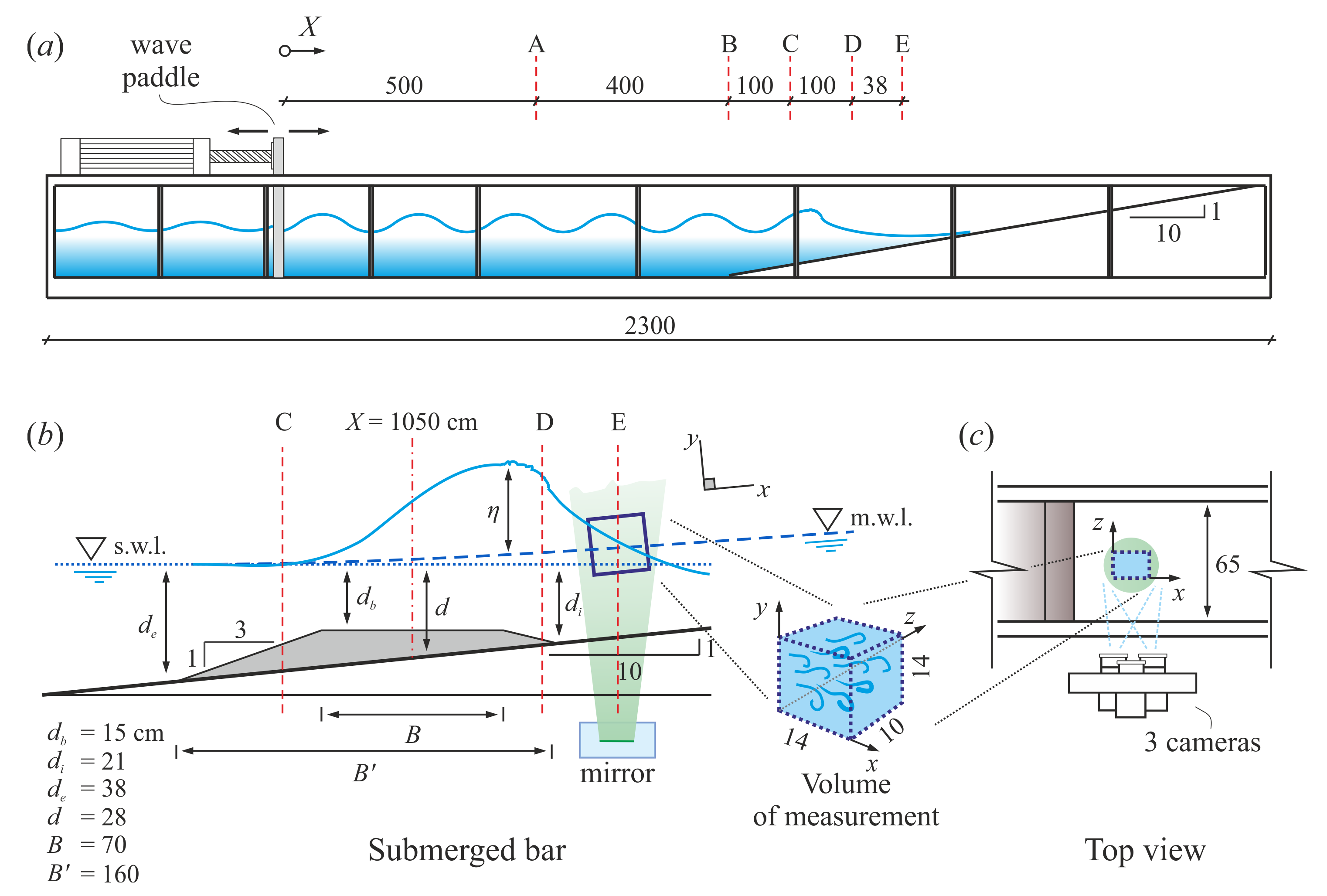
A series of experiments were planned in the wave flume of the Andalusian Institute for Earth System Research (IISTA), Universities of Granada and Cordoba, in Granada. An artificial slope of 1:10 with a berm of stones and plastic blocks was realized in order to force the breaking section, see Figure 1, with a still-water depth in front of the paddle of . Reflection was controlled with an active absorption system (AWACS).
A three-dimensional (3D) Particle Tracking Velocimetry system (V3V by TSI Inc., USA) was used for measuring the velocity in a volume of ≈14 . The volume of measurement was enlightened by a laser, and three cameras ( pixels) generated three pairs of 12-bit images, with a time delay between two images of each pair of . The frequency of V3V was , with 10 or 13 shots per each period for waves with and , respectively. Each experiment contained 10 cycles, with a total of 100 and 130 shots. The overall accuracy in velocity measurements is 0.1 cm/s for the cross-shore and the vertical direction, and 0.4 cm/s for the alongshore velocity component.
The surface elevation during tests was measured in several sections using Ultrasonic probes (UltraLab® USL 80D by General Acoustics, Kiel, Germany, sensor model USS635), with an accuracy on the instantaneous water level measurements equal to mm.
The main parameters of the experiments are listed in Table 1.
3. Data Analysis and Visualization
The raw signal was elaborated by applying operators expressing different kind of averages. The phase-average for the variable a is
where T is the period of the signal and N is the number of cycles. The time-average is defined as
and the phasic-average is defined as
where and if water is present or absent, respectively. The relative volume of water is and below the (minimum) trough level, and above the (maximum) crest level. The phasic-average is always greater than and equal to the time average if and , respectively.
The phasic-phase-average is also defined as
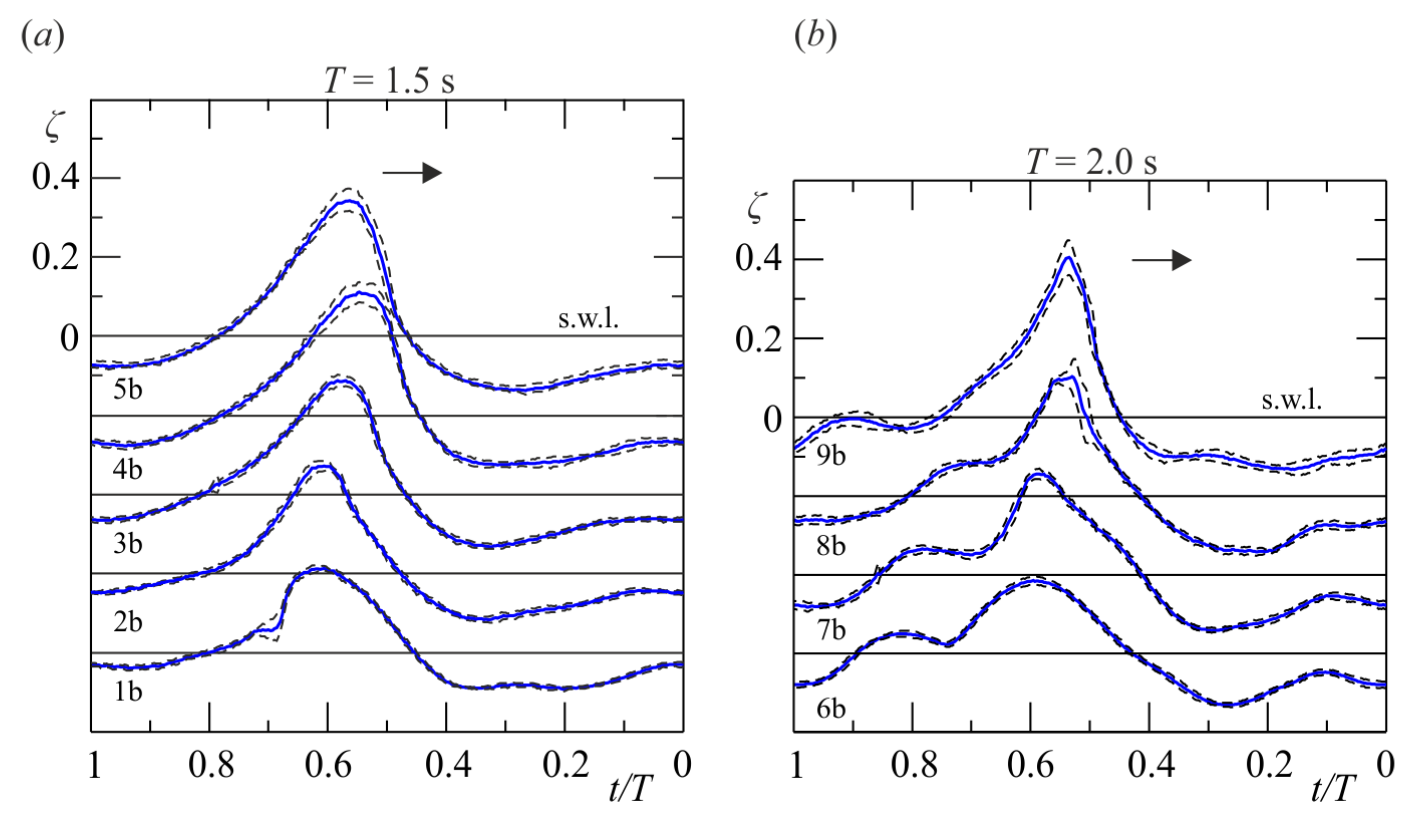
For simplicity and for more consistency, in the present analysis we refer to “vertically integrated” data, meaning data phasic-averaged in the vertical, and “cycle integrated” equivalent to a time-average or a phasic-average according to the indications. Figure 2 shows the shape of the wave at the breaking section for all the experiments.
The first problem is the separation of periodic (organized) components and fluctuating (turbulent) components. First (i) a principal orthogonal decomposition (POD) is applied to the time series of the spatial measured velocity in order to detect the most energetic contributions; (ii) then a cut-off number of components is chosen in order to eliminate disturbances and the reconstructed time series with a limited number of modes is used for the computations. The details are reported in Clavero et al., (2016) [16]. The results are presented as average in the cross-shore and alongshore directions, obtaining a single profile in the vertical per shot as average of ≈800 profiles. If the results are further phase averaged over 10 and 13 cycles, each profile in the vertical is the average of ≈8000 and ≈10,500 profiles, a very large sample which guarantees an adequate accuracy of the statistical estimators.
Figure 3 shows the instantaneous measured velocity, the phase-averaged and the fluctuating velocity for a single snapshot of Experiment 6b.
4. Turbulent Stress Invariants Analysis and Relation with the Dissipation Tensor
The anisotropy Reynolds stress tensor is defined as
where is the turbulent kinetic energy, are the spatial components and if , if is the Kronecker delta. Perfect isotropy gives a tensor with null diagonal elements.
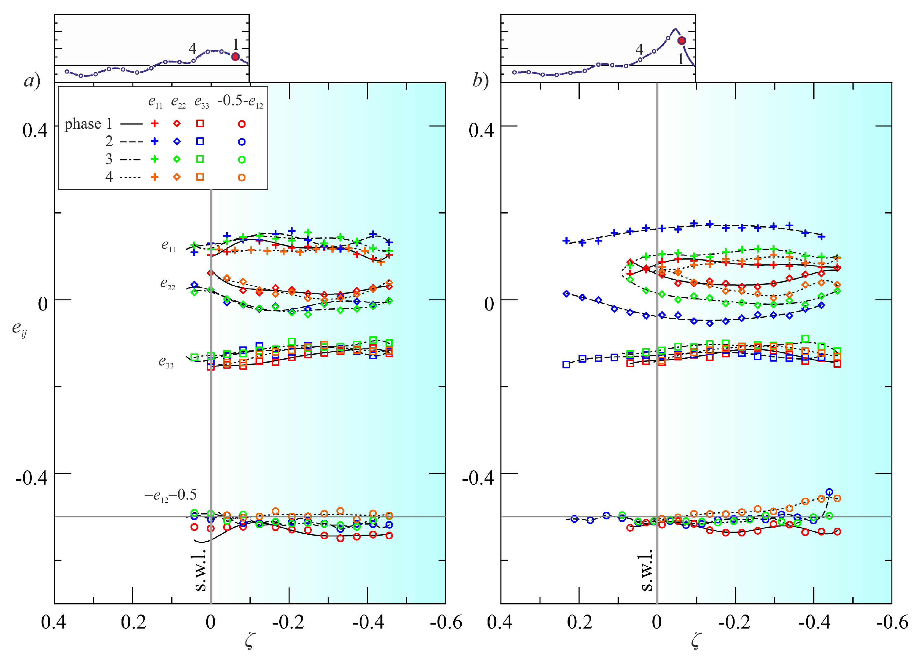
Figure 4a,b show the most representative elements for the four phases across breaking, for Experiment 6b and Experiment 9b, respectively (the less and the most energetic breaking conditions).
In Experiment 6b, turbulence is largely oriented in plane 1–2 (cross-shore-vertical), with the 3rd component (longshore) carrying a modest fraction of the total kinetic energy. The changes of the structure due to breaking are modest and mainly limited to an increment of turbulent kinetic energy (TKE) in the 3-direction. In Experiment 9b there is a clear evolution of the tensor before and after breaking. In phase 2 a significant axisymmetric structure develop with axis along the 3-direction.
A useful tool to analyse the structure of turbulence is given by the Lumley triangle, which contours all the Reynolds anisotropy stress tensor invariants (Lumley, 1978 [18]). For an incompressible flow, the three invariants of the anisotropy tensor are
and they are bounded by limits related to the state of turbulence. For instance, is the definition of isotropic turbulence; while represents one-component turbulence, and represents two-component turbulence. In most cases the modified expressions for the invariants, and , are adopted.
A different synthetic representation of the level of anisotropy of turbulence is obtained through the eigenvalues of the anisotropy Reynolds tensor. Let , and be the three eigenvalues in descending order, the tensor can be expressed as a linear combination of the three tensors of a basis (see Banerjee et al., 2007 [19]) with coefficients given by
and satisfying the normalizing condition . These coefficients are used to plot a barycentric map according to the following transformation (see Banerjee et al., 2007 [19])
where are the coordinates of three arbitrary basis points. Usually the barycentric map is an equilateral triangle.
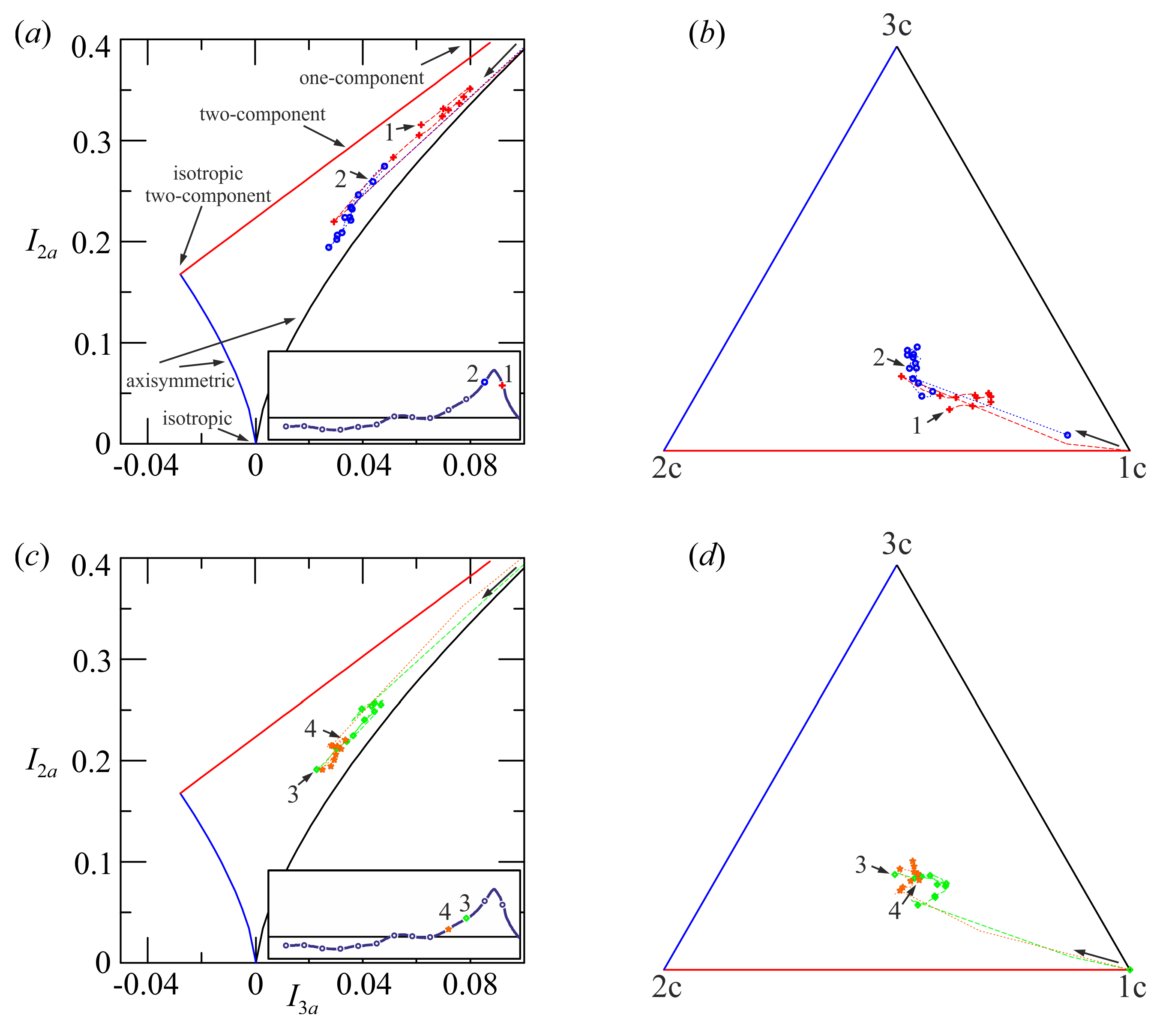
Figure 5 shows the structure of turbulence in Experiment 6b represented in a Lumley map and in a barycentric map, with data averaged in horizontal layers 0.4-cm thick, for the first four phases of the first wave cycle. Breaking appears between phase 2 and phase 3. In all of the analysed phases, turbulence has three different components and is anisotropic. At the wave crest and near the free surface, the turbulence is almost one-component turbulence, with only the cross-shore component.
Figure 6 shows the structure of turbulence in Experiment 9b, with breaking between phase 1 and phase 2. Again, turbulence is three-component and in general the distance from isotropy is smaller for the deepest levels, toward the bottom. An exception is phase 3, after breaking, in which the levels near the free surface have a degree of isotropy larger than that of the levels toward the bottom. The scenario is coherent with the turbulence in the breaker being mainly one dimensional (in the x direction) and with a fast return to isotropy. This fast return can be attributed partially to the fluctuating pressure acting to redistribute the energy amongst the three components, and partially to the transport toward the bottom of the most energetic components, which in turn are responsible of the increase in anisotropy in the deep layers. This mechanism of exchange of anisotropy between different vertical layers can be observed only for the highest waves of the set of experiments (Experiment 5b -not shown- and Experiment 9b) and is much less evident for the less energetic breakers.
An anisotropy measurement suggested by Lumley and Newman (1977) [20] is , which varies between for a two-component turbulence, and for the three-component isotropic turbulence. Figure 7 shows the invariant function F for two experiments, five phases across breaking, first cycle.
The flow organization reasonably influences the small scale turbulence structures, inducing isotropy or anisotropy in the dissipation rate (Antonia et al., 1994 [21], Mansour et al., 1988 [22]). The structure of dissipation rate is depicted by the following tensor
with its anisotropic form
where is the kinematic viscosity and is the average dissipation rate of TKE.
This tensor has been considered as a significant element in the attempts to model Reynolds stresses, since and are likely to be related at least in some categories of flow. Figure 8 show the main components of the anisotropic dissipation tensor for two experiments. Again for the most intense breaking wave the dissipation tensor is largely anisotropic, with the main term in the cross shore direction immediately after breaking. The overall relation between the two tensors is depicted in Figure 9, where the invariant function F for the anisotropy Reynolds tensor is compared with the corresponding invariant for the anisotropy dissipation tensor . For Experiment 1b–6b (low energy breaking) there is a proportionality between F and , with dissipation more isotropic () than turbulence, and with . For Experiments 5b–9b (high energy breaking) the data are much more dispersed. The dissipation tensor is still more isotropic than turbulence, but there is no evident correlation with the level of isotropy of turbulence tensor. Surprisingly, the coherence is still present only for data measured above the still water, in the breaker crest. All these analyses refer to macroturbulence, since the data resolution in space and time of the measurements does not allow an in-depth analysis of the behaviour at the microscales.
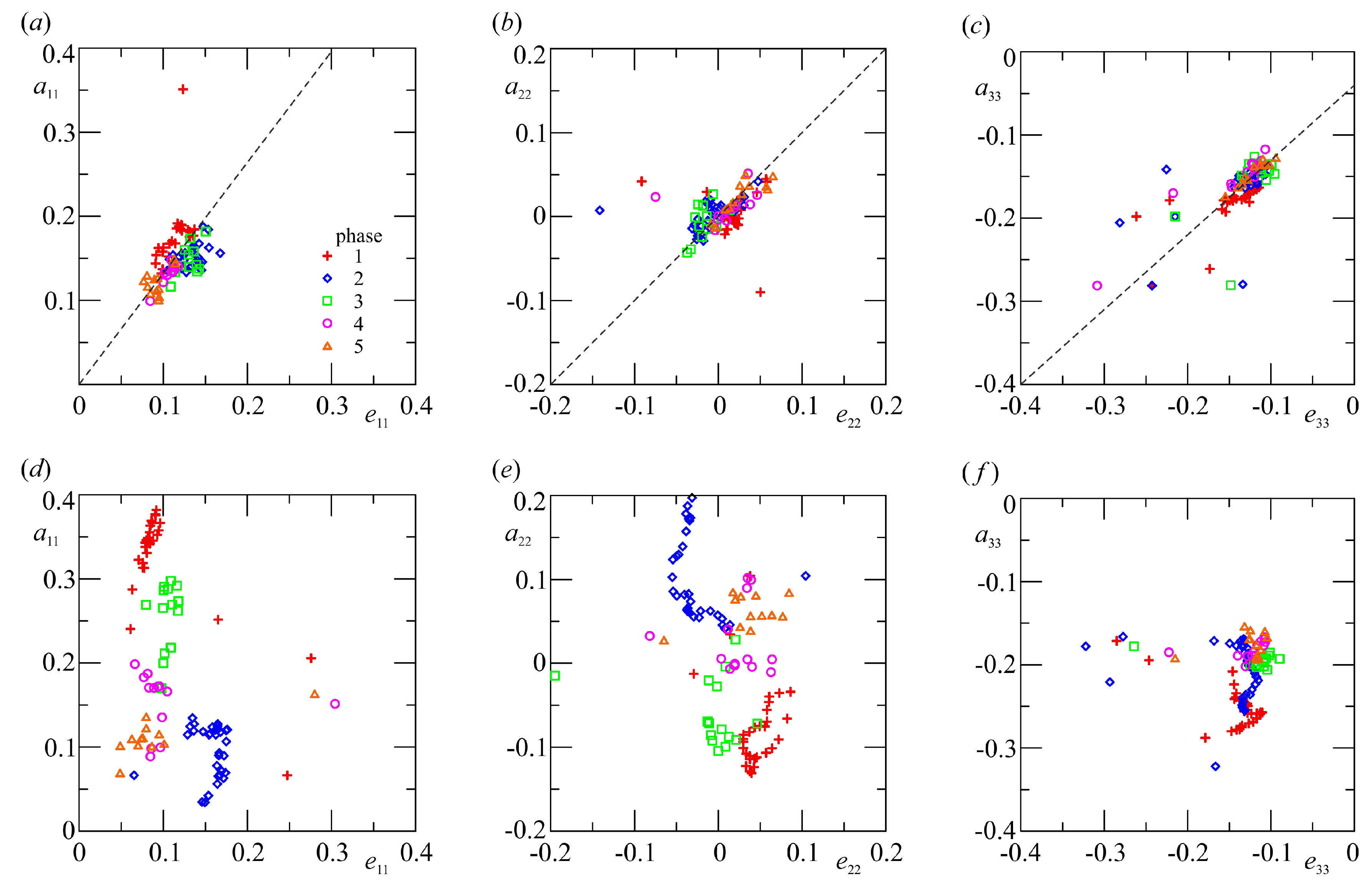
Several data in literature show that a relationship holds between the components of the anisotropy Reynolds tensor and of the anisotropy dissipation tensor. The shape of the relation is strictly dependent on the flow field and has been described as linear in wall boundary layer (see Antonia et al., 1994 [21]). Also in the present experiments a linear function is forecast for the low energy breaker in Figure 10a–c, with a coefficient of proportionality almost equal for the three main components. We expect that the coefficient is function of the ratio between the turbulence microscale and the integral macroscale (see, e.g., Tennekes and Lumley, 1972 [23], Longo, 2010 [15]), which in the present experiments is related to the intensity of the breaker. However, very energetic breakers show a poor coherence between the components of the two tensors, see Figure 10d–f.
5. Conclusions
We have analysed the anisotropy of the Reynolds stress and of the dissipation tensors with a unique dataset of measurements in breaking waves. The anisotropy is quantified by the invariants and is relatively high during all phases and more evident for the most energetic breakers. For low energy breakers, anisotropy is minor in the dissipation tensor than in the Reynolds stress tensor, with ( means perfect isotropy). For high energy breakers, the dissipation tensor still has an adequate level of isotropy, the Reynolds stress tensor is biased toward anisotropy.
The relationship between the main components of the two tensors is a simple proportionality for low energy breaker. That means that some classical models of turbulence are still applicable. For high energy breakers the relationship looks much more complex, and no simple model can be suggested.
The unique availability of these experimental data has allowed an in depth analysis following the same path adopted for DNS data. However, we expect that the dissipation tensor is affected by the limited space resolution of the data, and both tensors are affected by the limited time resolution, hence the presented results should be evaluated in the light of these limitations.
Beyond the application of well known models for turbulence estimation, there is the important novelty of huge experimental data set for calibrating these models. This data set are a step ahead toward the detailed interpretation of the fundamental mechanisms of turbulence generation, evolution and dissipation.
As a development of data analysis there is the evaluation of the “dimensionality” elements of turbulence. This is left to future work.
Author Contributions
S.L. and L.C. conceived and designed the experiments and performed the experiments with M.C.; S.L., L.C., M.C. and M.A.L. analyzed the data and wrote the paper.
Conflicts of Interest
The authors declare no conflict of interest.
References
- Longuet-Higgins, M. Capillary rollers and bores. J. Fluid Mech. 1992, 240, 659–679. [Google Scholar] [CrossRef]
- Lin, J.; Rockwell, D. Instantaneous structure of a breaking wave. Phys. Fluids 1994, 6, 2877–2879. [Google Scholar] [CrossRef]
- Dabiri, D.; Gharib, M. Experimental investigation of the vorticity generation within a spilling water wave. J. Fluid Mech. 1997, 330, 113–139. [Google Scholar] [CrossRef]
- Grue, J.; Kolaas, J. Experimental particle paths and drift velocity in steep waves at finite water depth. J. Fluid Mech. 2017, 810. [Google Scholar] [CrossRef]
- Smith, L.; Jensen, A.; Pedersen, G. Investigation of breaking and non-breaking solitary waves and measurements of swash zone dynamics on a 5∘ beach. Coast. Eng. 2017, 120, 38–46. [Google Scholar] [CrossRef]
- Barthelemy, X.; Banner, M.L.; Peirson, W.L.; Fedele, F.; Allis, M.J.; Dias, F. On the local properties of highly nonlinear unsteady gravity water waves. Part 2. Dynamics and onset of breaking. arXiv, 2015; arXiv:1508.06002v1. [Google Scholar]
- Saket, A.; Peirson, W.L.; Banner, M.L.; Barthelemy, X.; Allis, M.J. On the threshold for wave breaking of two-dimensional deep water wave groups in the absence and presence of wind. J. Fluid Mech. 2017, 811, 642–658. [Google Scholar] [CrossRef]
- Deike, L.; Melville, W.K.; Popinet, S. Air entrainment and bubble statistics in breaking waves. J. Fluid Mech. 2016, 801, 91–129. [Google Scholar] [CrossRef]
- Deike, L.; Pizzo, N.; Melville, W.K. Lagrangian transport by breaking surface waves. J. Fluid Mech. 2017, 829, 364–391. [Google Scholar] [CrossRef]
- Drazen, D.A.; Melville, W.K.; Lenain, L. Inertial scaling of dissipation in unsteady breaking waves. J. Fluid Mech. 2008, 611, 307–332. [Google Scholar] [CrossRef]
- Drazen, D.A.; Melville, W.K. Turbulence and mixing in unsteady breaking surface waves. J. Fluid Mech. 2009, 628, 85–119. [Google Scholar] [CrossRef]
- Reynolds, W.C. Effects of rotation on homogeneous turbulence. In Proceedings of the 10th Australasian Fluid Mechanics Conference, Melbourne, Australia, 11–15 December 1989; Volume 1, pp. KS2.1–KS2.6. [Google Scholar]
- Stylianou, F.; Pecnik, R.; Kassinos, S. A general framework for computing the turbulence structure tensors. Comput. Fluids 2015, 106, 54–66. [Google Scholar] [CrossRef] [Green Version]
- Robinson, S.K. Coherent motions in the turbulent boundary layer. Annu. Rev. Fluid Mech. 1991, 23, 601–639. [Google Scholar] [CrossRef]
- Longo, S. Experiments on turbulence beneath a free surface in a stationary field generated by a Crump weir: Free surface characteristics and the relevant scales. Exp. Fluids 2010, 49, 1325–1338. [Google Scholar] [CrossRef]
- Clavero, M.; Longo, S.; Chiapponi, L.; Losada, M. 3D flow measurements in regular breaking waves past a fixed submerged bar on an impermeable plane slope. J. Fluid Mech. 2016, 802, 490–527. [Google Scholar] [CrossRef]
- Chiapponi, L.; Cobos, M.; Losada, M.A.; Longo, S. Cross-shore variability and vorticity dynamics during wave breaking on a fixed bar. Coast. Eng. 2017, 127, 119–133. [Google Scholar] [CrossRef]
- Lumley, J. Computational modelling of turbulent flows. Adv. Appl. Mech. 1978, 18, 123–176. [Google Scholar]
- Banerjee, S.; Krahl, R.; Durst, F.; Zenger, C. Presentation of anisotropy properties of turbulence, invariants versus eigenvalue approaches. J. Turbul. 2007, 8, N32. [Google Scholar] [CrossRef]
- Lumley, J.L.; Newman, G.R. The return to isotropy of homogeneous turbulence. J. Fluid Mech. 1977, 82, 161–178. [Google Scholar] [CrossRef]
- Antonia, R.A.; Djenidi, L.; Spalart, P.R. Anisotropy of the dissipation tensor in a turbulent boundary layer. Phys. Fluids 1994, 6, 2475–2479. [Google Scholar] [CrossRef]
- Mansour, N.N.; Kim, J.; Moin, P. Reynolds-stress and dissipation-rate budgets in a turbulent channel flow. J. Fluid Mech. 1988, 194, 15–44. [Google Scholar] [CrossRef]
- Tennekes, H.; Lumley, J. A First Course in Turbulence; Cambridge University Press: Cambridge, UK, 1972. [Google Scholar]
Figure 1.
The experimental flume adopted for the tests: (a) side view of the flume; (b) layout of the bar and of the volume of measurement; (c) top view showing the cameras of the V3V system. The still water depth in the mid section of the bar ( cm) is cm. The dot line indicates the still water level, the dashed line is the mean water level (wave set-up or set-down). Dimensions are in centimeters.

Figure 2.
Wave profiles in the section of velocity measurements (Section D) for (a) the tests with , and (b) the tests with . The dashed lines limit the standard deviation band for the sample of 10 wave cycles during velocity acquisition.
Figure 2.
Wave profiles in the section of velocity measurements (Section D) for (a) the tests with , and (b) the tests with . The dashed lines limit the standard deviation band for the sample of 10 wave cycles during velocity acquisition.

Figure 3.
Experiment 6b, a single snapshot in a sequence of 13 shots of the first measured wave cycle. (a) Instantaneous velocity in the midplane of the flume (z = 0); (b) phase-averaged velocity; (c) velocity vectors difference (fluctuating velocity) between the instantaneous velocity and the phase-averaged velocity. Only velocity components in the x–y plane are shown. The inset depicts the surface elevation time series, with the symbols indicating the time of the shot. (modified from Clavero et al., 2016 [16], with permission).

Figure 4.
The main elements of the anisotropy tensor for four phases across breaking. (a) Experiment 6b; (b) Experiment 9b. The element is shifted downward, and only one experimental data of two is shown for an easy visualization.
Figure 4.
The main elements of the anisotropy tensor for four phases across breaking. (a) Experiment 6b; (b) Experiment 9b. The element is shifted downward, and only one experimental data of two is shown for an easy visualization.
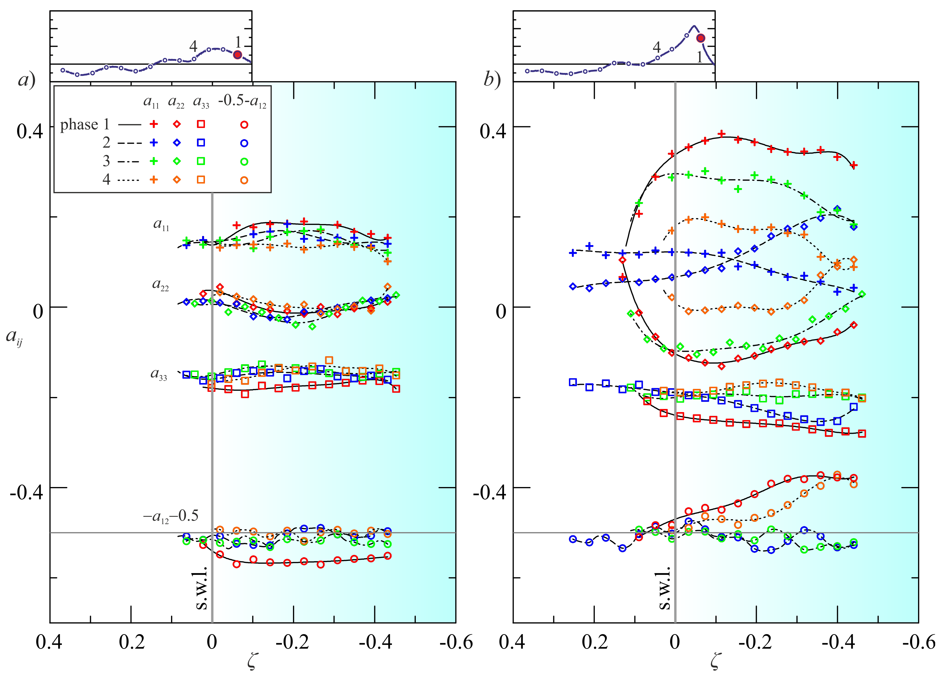
Figure 5.
Experiment 6b, first four phases (crosses, circles, squares and stars), first wave cycle. (a–c) Lumley map; (b–d) barycentric map based on scalar metrics which are functions of eigenvalues of the second order stress tensor describing turbulence. The values are averaged in horizontal layers. The insets show the phase, the arrows indicate the deepest point, with data 0.4 cm apart. Only one point of three is plotted for a clear visualization.
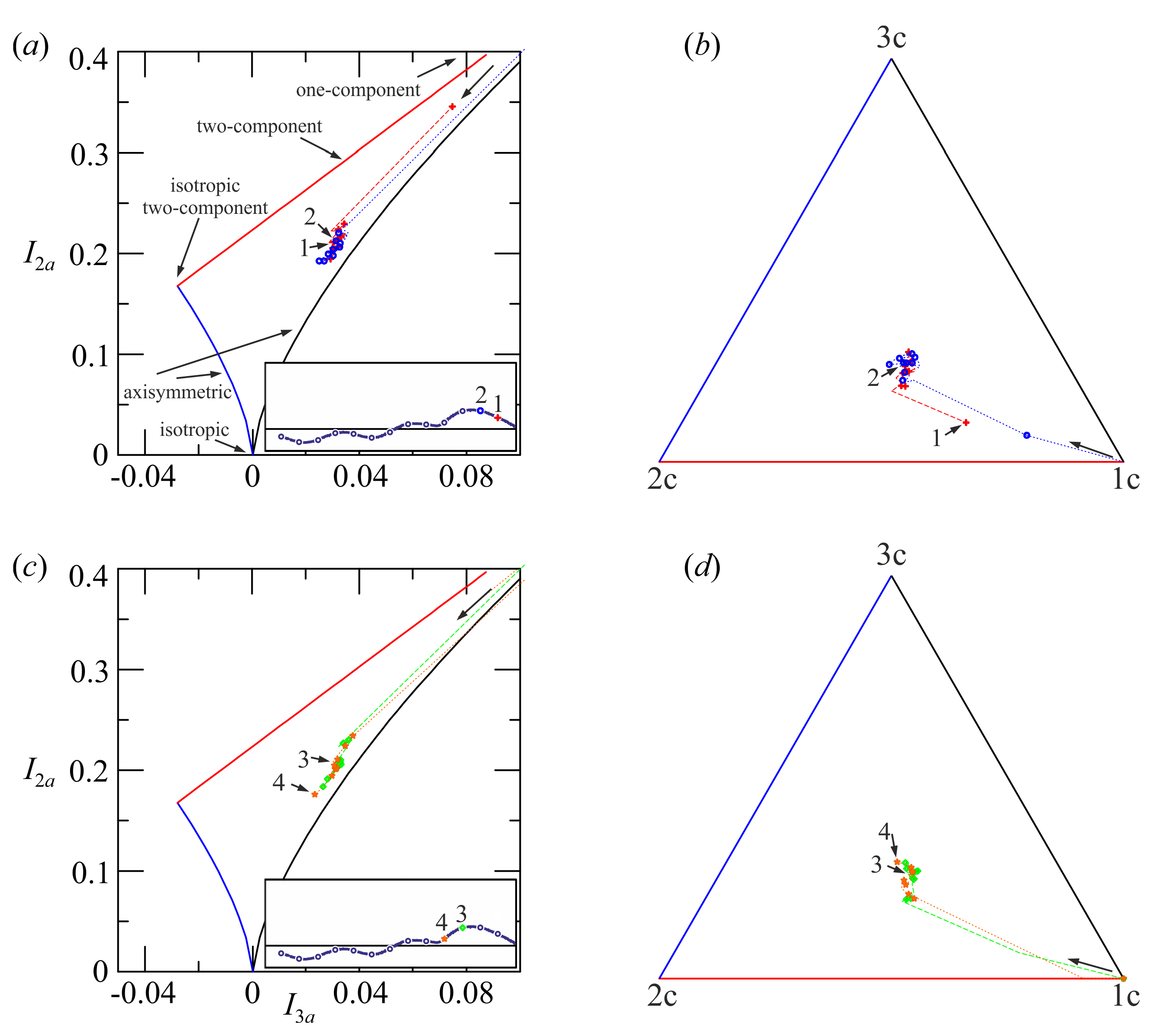
Figure 6.
Experiment 9b, see Figure 5 for caption.
Figure 6.
Experiment 9b, see Figure 5 for caption.

Figure 7.
Invariant function for the first five phases. (a) Experiment 6b; (b) Experiment 9b.
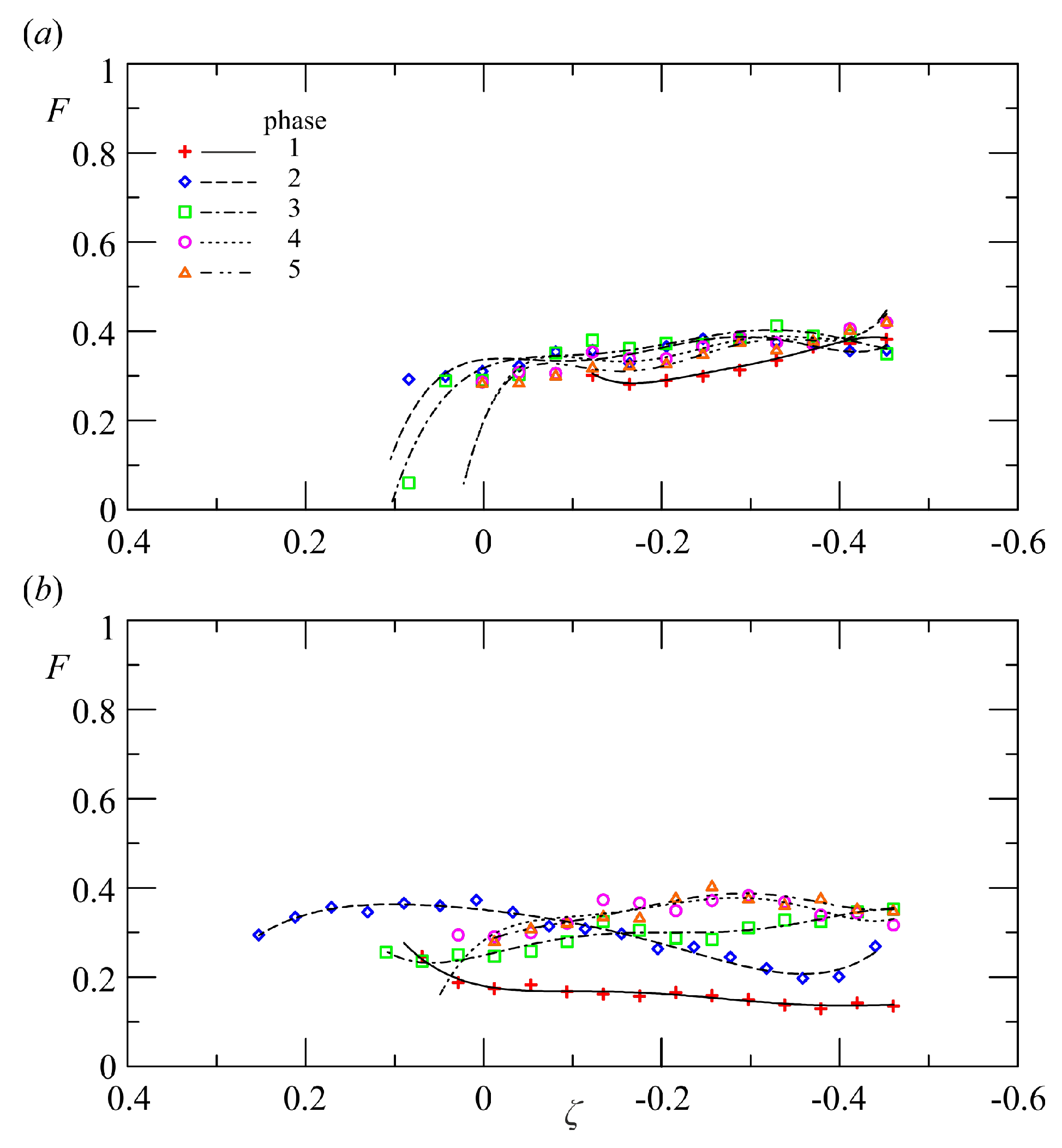
Figure 8.
The main elements of the dissipation anisotropy tensor for four phases across breaking. (a) Experiment 6b; (b) Experiment 9b. The element is shifted downward, and only one experimental data of two is shown for an easy visualization.
Figure 8.
The main elements of the dissipation anisotropy tensor for four phases across breaking. (a) Experiment 6b; (b) Experiment 9b. The element is shifted downward, and only one experimental data of two is shown for an easy visualization.

Figure 9.
Comparison of the invariant function of the turbulence and of the dissipation tensors for the first five phases. (a) Experiment 1b; (b) Experiment 2b; (c) Experiment 6b; (d) Experiment 9b. The dashed curve is the interpolating line. Gray symbols refer to measurements above the still water level.
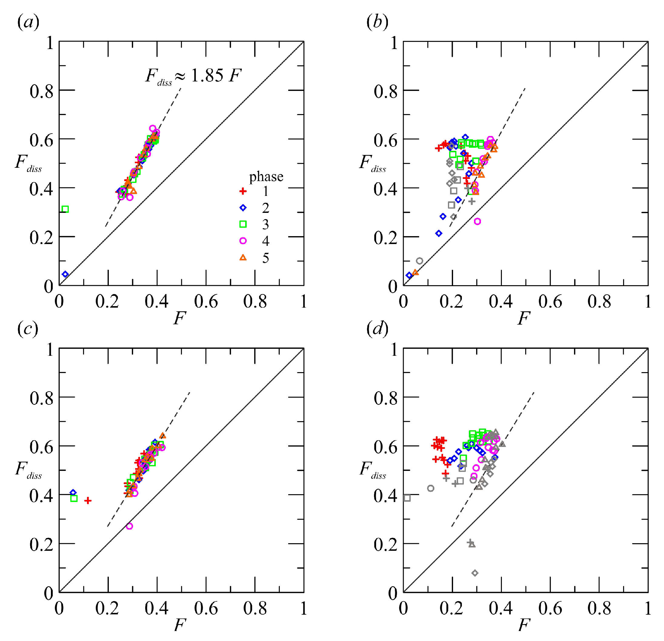
Figure 10.
Relation between and . (a–c) Experiment 6b; (d–f) Experiment 9b. The dashed curves are the interpolating lines.
Figure 10.
Relation between and . (a–c) Experiment 6b; (d–f) Experiment 9b. The dashed curves are the interpolating lines.

Table 1.
Parameters of the tests. is the target wave height (almost coincident with the generated wave height), T is the wave period and is the deep-water wave steepness. is the Iribarren number ( is the bed slope), is the mean water depth in the section of measurements, is the wave set-up, and , , and are the root-mean-square wave height, the mean of the highest third of the waves, and the maximum wave height, respectively, all referred to as the statistics of the breakers. and are the still-water depth at the internal and external toe of the bar, respectively, B and are the width of the crest and the total width of the bar. The still-water depth in front of the paddle is 43 cm and the breaking section is D at cm, with a still-water depth cm.
| Exp. | (cm) | T (s) | h (cm) | (cm) | (cm) | (cm) | (cm) | ||||||
|---|---|---|---|---|---|---|---|---|---|---|---|---|---|
| 1b | 6 | 1.5 | 0.017 | 0.765 | 19.2 | 0.0 | 5.7 | 6.2 | 6.3 | 0.060 | 0.109 | 0.199 | 0.456 |
| 2b | 7 | 1.5 | 0.020 | 0.708 | 19.4 | 0.2 | 7.4 | 8.1 | 8.7 | ||||
| 3b | 8 | 1.5 | 0.023 | 0.662 | 19.6 | 0.4 | 8.0 | 8.6 | 8.8 | ||||
| 4b | 9 | 1.5 | 0.026 | 0.624 | 19.7 | 0.5 | 8.7 | 9.2 | 9.9 | ||||
| 5b | 10 | 1.5 | 0.028 | 0.592 | 19.8 | 0.6 | 9.2 | 9.9 | 10.4 | ||||
| 6b | 6 | 2 | 0.010 | 1.020 | 19.4 | 0.2 | 6.1 | 6.3 | 6.5 | 0.034 | 0.061 | 0.112 | 0.256 |
| 7b | 7 | 2 | 0.011 | 0.944 | 19.4 | 0.2 | 7.6 | 8.3 | 8.7 | ||||
| 8b | 8 | 2 | 0.013 | 0.883 | 19.5 | 0.3 | 9.0 | 9.6 | 10.4 | ||||
| 9b | 9 | 2 | 0.014 | 0.833 | 19.6 | 0.4 | 10.3 | 11.2 | 12.8 |
© 2017 by the authors. Licensee MDPI, Basel, Switzerland. This article is an open access article distributed under the terms and conditions of the Creative Commons Attribution (CC BY) license (http://creativecommons.org/licenses/by/4.0/).
Share and Cite
MDPI and ACS Style
Longo, S.; Clavero, M.; Chiapponi, L.; Losada, M.A. Invariants of Turbulence Reynolds Stress and of Dissipation Tensors in Regular Breaking Waves. Water 2017, 9, 893. https://doi.org/10.3390/w9110893
AMA Style
Longo S, Clavero M, Chiapponi L, Losada MA. Invariants of Turbulence Reynolds Stress and of Dissipation Tensors in Regular Breaking Waves. Water. 2017; 9(11):893. https://doi.org/10.3390/w9110893
Chicago/Turabian StyleLongo, Sandro, Maria Clavero, Luca Chiapponi, and Miguel A. Losada. 2017. "Invariants of Turbulence Reynolds Stress and of Dissipation Tensors in Regular Breaking Waves" Water 9, no. 11: 893. https://doi.org/10.3390/w9110893
Note that from the first issue of 2016, this journal uses article numbers instead of page numbers. See further details here.