Effect of Water Quality Sampling Approaches on Nitrate Load Predictions of a Prominent Regression-Based Model

Abstract

High frequency in-situ measurements of nitrate can greatly reduce uncertainty in nitrate flux estimates. Water quality databases maintained by various federal and state agencies often consist of pollutant concentration data obtained from periodic grab samples collected from gauged reaches of a stream. Regression models, such as the LOAD ESTimator (LOADEST), are frequently used to model variations in concentrations associated with changes in water discharge to provide integrated solute flux measurements. However, uncertainty in the relationships between nutrient concentration and flow may lead to errors in the corresponding flux estimates. In this study, a high frequency, in-situ measurement of nitrate concentration was implemented to ascertain uncertainty in the concentration/discharge relationship caused by nitrate hysteresis. It was found that observed nitrate hysteresis, as influenced by complex storm/watershed interactions, was not readily predictable. Therefore, it can lead to substantial nitrate flux uncertainty, based on periodic grab sample monitoring approaches. Scientists and engineers should take advantage of the proposed findings in future studies to enhance the quality of the associated decision making processes.

1. Introduction

Water quality variables, such as stream nutrient and sediment concentrations, are often used to assess the condition of a waterbody and to evaluate trends in constituent loadings over time. Collecting and analyzing water quality samples can be resource intensive. Therefore, sampling frequency may vary based on the availability of potentially limited resources (such as budgets and personnel). In general, water quality measurements are conducted by sparse and periodically-collected grab samples. On the other hand, the fact that water quality data are usually discontinuous in time may cause some technical difficulties in the application of relevant work such as watershed modeling, which requires temporally-continuous monitoring. Therefore, regression-based models such as the Support Vector Regression and Regression Trees [1], and the LOAD ESTimator (LOADEST) [2,3], among others [4,5,6,7,8,9], have been developed to produce more temporally-continuous datasets. LOADEST is a commonly adopted program used to estimate constituent loads in rivers and streams [10,11,12,13,14,15]. With LOADEST, discrete water quality sample concentrations can be converted to finer time scales by using continuous streamflow data. Due to its simplicity of practical operation and diverse options (i.e., built-in models), LOADEST has been widely used to estimate daily and monthly constituent loads for various water quality parameters with various sampling frequencies (i.e., weekly, bi-weekly, monthly, or bi-monthly) [12,13,14]. LOADEST provides users the option of automatically selecting a regression model that best suits the given dataset or choosing one of several built-in regression models for the estimation of constituent loads [15].

A limitation of LOADEST, however, is that the regression model is sensitive to the assumption of a fixed/stationary concentration-flow relationship and does not account for changes or trends in the concentration-flow relationship (hysteresis). This drawback can potentially be resolved mathematically by using equations with more variables. However, this raises the chances of over fitting and compromising the regionalized data (after regression analysis). On the other hand, changes in storm hydrographs are typically associated with a lag effect in streamflow constituent concentration, resulting in hysteresis loops [16,17]. Positive hysteresis occurs in the form of a clockwise loop when constituent concentrations on the rising limb of a storm hydrograph are higher than those measured at equivalent flows on the falling limb. If the constituent concentrations are higher on the falling limb, the hysteresis will run counterclockwise [18]. Predicted discharge versus constituent concentration rating curves may have a high degree of uncertainty [19], as hysteresis effects are almost always present and difficult to predict. Hysteresis influence on the hydrograph is especially pronounced during extremely high flows [20], often resulting in the estimate for a particular day being unrepresentative of the actual loads. In general, the use of data from fixed-interval, time-based sampling is not appropriate for constituent load estimation. In addition, the effect of hysteresis and the associated uncertainty are not accounted for by the models used in LOADEST. Therefore, to adequately estimate constituent loads using LOADEST, it is suggested that the monitoring programs providing data for LOADEST should be managed to effectively capture the entire range of flow conditions [20,21].

It has been stated in the literature that measurement uncertainty may have substantial impacts on model predictions [22,23]. Therefore, it is important to improve the quality of measurement data to enhance the credibility of the following data-used applications (such as watershed modeling, decision making processes, etc.). Real-time monitoring (in-situ sampling) provides an alternative to the typical monthly or bimonthly sampling techniques (e.g., grab sampling and on-site sampling) used in long-term water quality monitoring programs. Data can be collected more frequently, in smaller time steps, with the results being accessible remotely once the sampling equipment is installed. Advances in in-situ nitrate sensors provide an opportunity to measure changes in nitrate concentration at higher frequencies (often sub-hourly) [24]; such advances have been useful in real-time monitoring of water quality and nitrogen dynamics [25,26]. Real-time nitrate sampling may improve the accuracy and precision of load estimates by reducing sample bias and uncertainty inherent in data derived from regression models that are subject to hysteresis effects.

The primary goal of this study was to investigate the applicability of the proposed approach by using a well-recognized regression model. Specifically, the following objectives were defined: (i) to examine whether a regression model calibrated with samples covering the whole range of hydrologic flows/conditions may outperform similar models, calibrated with a dataset that only covers specific hydrologic conditions; and (ii) to explore the effects of hysteresis on nitrate delivery and load prediction errors in the targeted watershed.

In this study, we took advantage of a real-time, in-situ nitrate dataset to investigate the effects of sampling time and frequency on LOADEST storm loading predictions in a Mid-Atlantic watershed that has a rich database of historic water quality samples, as well as a real-time monitoring dataset. As stated previously, the general recommendation for collecting water quality samples is to cover the entire range of flows/conditions at different stages of the hydrograph (i.e., rising limb, falling limb, peak flow, and baseflow) [27]. We hypothesized that when hysteresis is presented in the concentration-flow relationship, it may not be the best strategy to sample different stages of the hydrograph; rather, it would be better to focusing sampling efforts on the section of the hydrograph delivering the largest loads. We tested this hypothesis by constructing various regression models that share a single form (type) but are calibrated using different water quality sample sets. These sample sets come from a database of water quality samples that were taken at different stages of the hydrograph and grouped based on the corresponding time of sampling. Ultimately, the regression models were validated against real-time, observed water quality data. The uncertainty of the regression relationships was gauged and considered during the validation of each regression model. To test our hypothesis, we used nitrate data collected from Greensboro watershed, which is a mid-sized, mixed land use (forest and agriculture) watershed on the eastern shore of Chesapeake Bay.

2. Materials and Methods

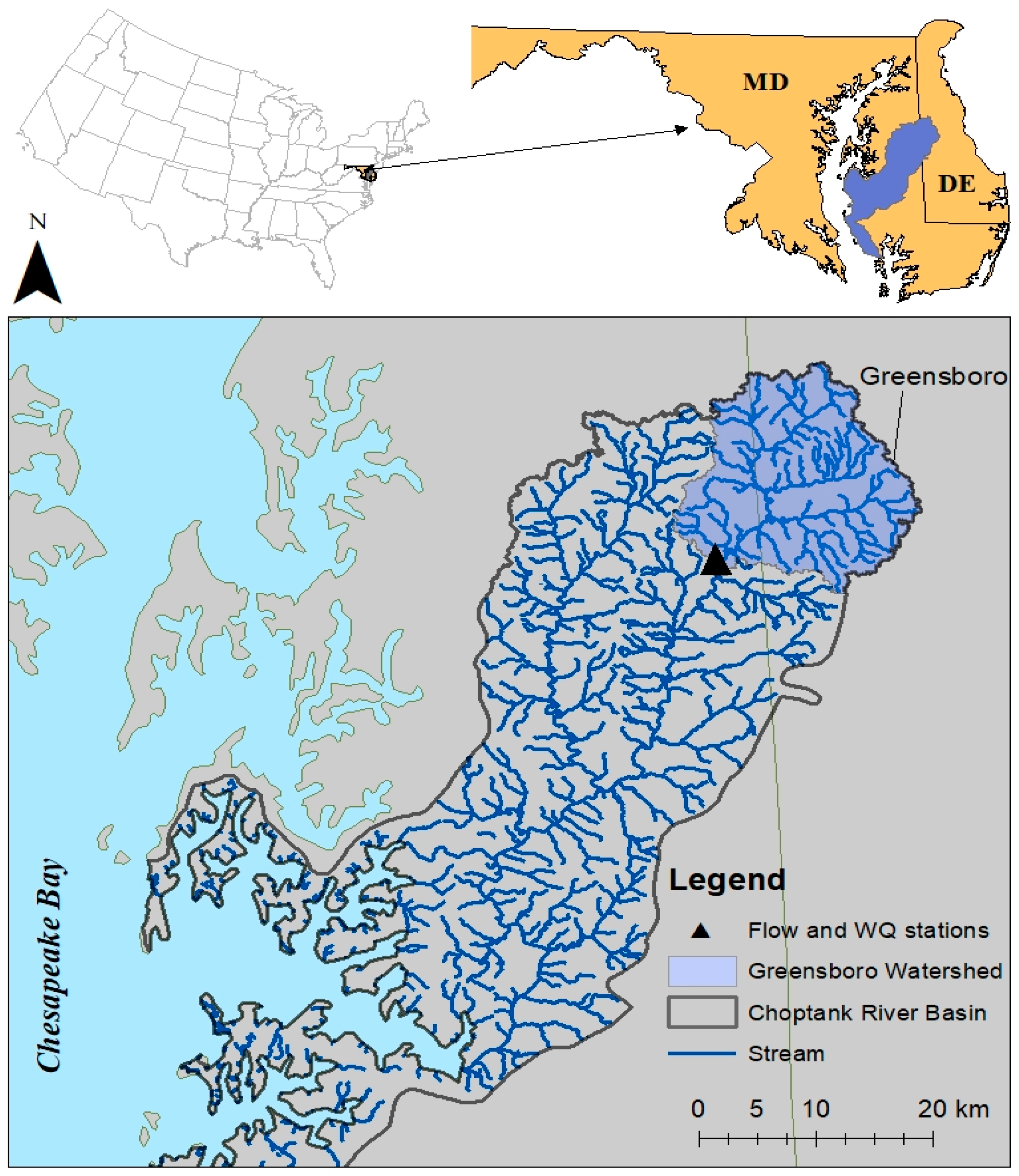
2.1. Study Area

The Greensboro watershed is part of the Choptank River basin on the Eastern Shore of Chesapeake Bay (Figure 1). The Greensboro watershed originates in Kent County, Delaware, extending southwest towards the township of Greensboro, Caroline County, Maryland. The drainage area for the Greensboro watershed is approximately 290 km² and is comprised of 48% forested land and 36% agricultural fields. Average annual precipitation and temperature for the study region is 1120 mm and 13.3 °C, respectively.

The Choptank River has been classified as “impaired waters” under the Clean Water Act (USEPA, 2010) for excessive nutrient and sediment loads. It is estimated that agriculture accounts for ~80% of the Choptank’s nutrient loadings (nitrogen and phosphorus) to the Chesapeake Bay; roughly 60% of the watershed area is covered by agriculture [28]. For this reason, the Choptank River Basin and the nearby regions have been the focus of multiple federal studies, including the U.S. Department of Agriculture (USDA)—Conservation Effects Assessment Project (CEAP) and the USDA Long-term Agro-ecosystem Research (LTAR) Network [29,30]. This has led to extensive research and monitoring projects within the basin in recent years. Baseflow constitutes approximately 64% of Choptank’s streamflow (estimated using the baseflow separation tool [31]) and acts as a principal mechanism for delivery of nitrogen to the Chesapeake Bay. Studies have found that up to 70% of nitrate flux in the region’s surface waters is transported via base flow [27,28].

2.2. Historic Discharge and Water Quality Sampling Data

At the outlet of the Greensboro watershed (Lat 38°59′49.9′′, long 75°47′08.9′′), there is a gauging station operated by the U.S. Geological Survey that has monitored a section of the Choptank River since January 1948. USGS has also collected water quality samples (including nitrate) at the same gauging station since June 1964. As of October 2007, river discharge has been recorded at a much higher temporal resolution (15-min interval) compared to the earlier period (daily). Availability of the higher resolution discharge data enabled us to visually inspect and separate water quality samples based on the time of sampling in respect to the state of the hydrograph (rising/falling limbs of flow curves). In other words, USGS nitrate samples were divided into three separate groups: baseflow samples, rising samples, and falling samples. Samples were classified as baseflow on occasions when baseflow constituted 90% of total streamflow, as suggested in [32]. Baseflow separation was performed using the Web-based Hydrograph Analysis Tool (WHAT) [31].

During October 2007 and June 2016, 454 nitrate samples were analyzed by USGS, among which 291 samples were taken during baseflow periods (64%); 100 were rising samples (22%), and 63 were falling samples (14%). Using the three groups, five separate calibration databases were constructed to include all the samples (All, n = 454), baseflow + rising samples (Base-Rising, n = 391), baseflow + falling samples (Base-Falling, n = 354), only rising samples (Rising, n = 100) and only falling samples (Falling, n = 63). These five databases were then used to fit regression models in LOADEST, which were subsequently validated against observed real-time nitrate data at the outlet of Greensboro watershed.

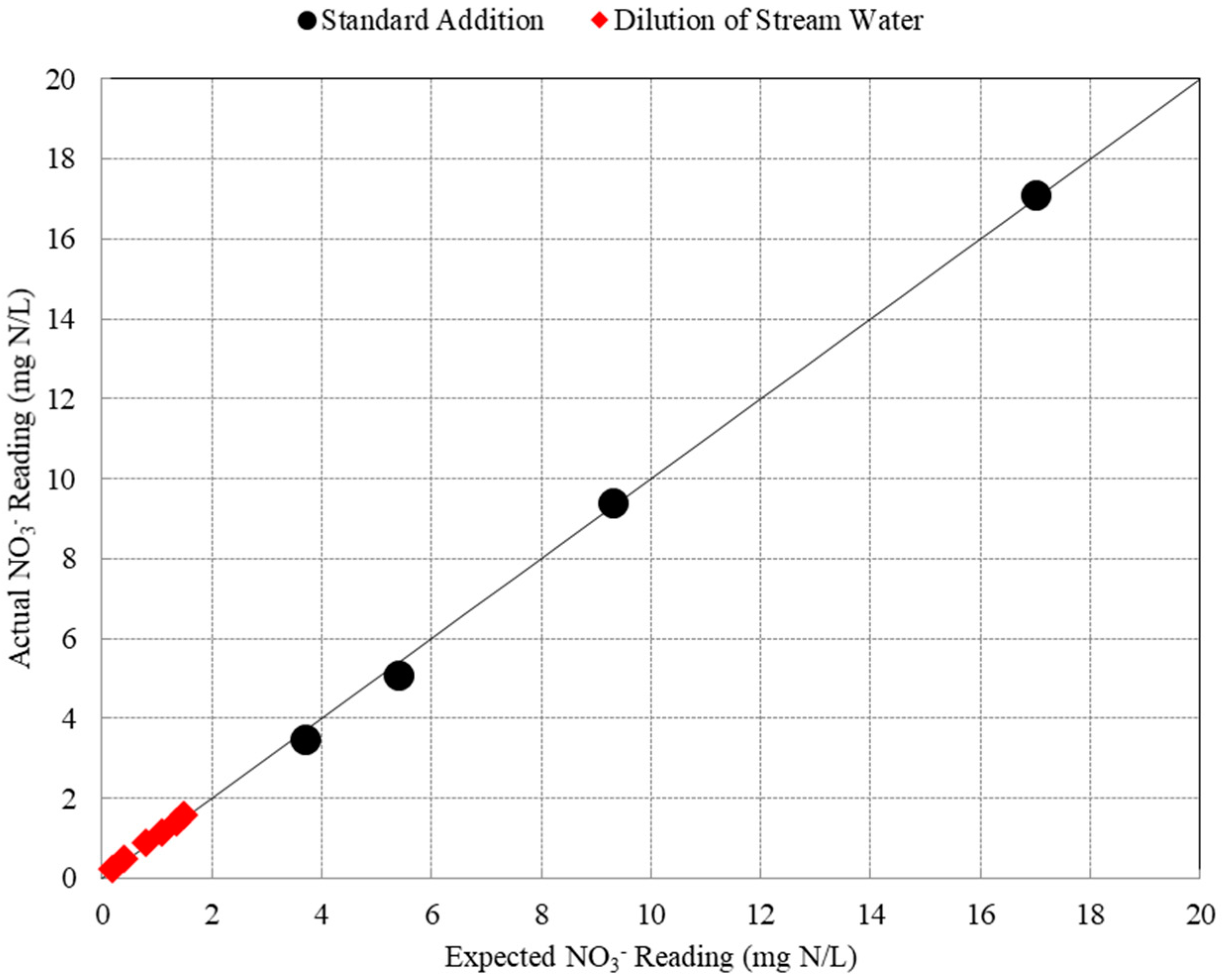
2.3. Real-Time Nitrate Data Processing

Researchers at the U.S. Department of Agriculture–Agricultural Research Service (USDA–ARS) have been performing continuous nitrate data collection at 30-min intervals at the outlet of Greensboro watershed since the summer of 2014. In-situ measurements of nitrate concentrations were performed using a full spectrum (200 to 700 nm) spectrometer probe (S-CAN spectrolyser probe, Vienna, Austria) with 15 mm path length and fitted with a flow cell. Stream water was automatically sampled on a 30-min interval by use of a peristaltic pump connected to the flow cell.

The stability of sensor for the global nitrate calibration in natural water was tested by adding known amounts of nitrate to the Greensboro water sample and verified by comparing sensor readings. In addition, some water samples were diluted with known amounts of distilled water to be tested with the sensor. As shown in Figure 2, calibration results exhibited a linear, one to one relationship between actual and sensor concentrations (slope = 1.02, not significantly different from 1). The observation period ranged from June 2014 to June 2016. The high-resolution nitrate concentration data were multiplied by USGS collected stream discharge to construct a time series of nitrate loading at the outlet of Greensboro watershed (Figure 3).

2.4. USGS LOAD ESTimator

LOADEST is a regression-based program, commonly employed to convert discontinuous, periodic (weekly, monthly) grab sample concentration measurements into a continuous (hourly, daily) time series. Using LOADEST, one can construct a regression model for estimation of constituent load, based on given time series of discharge, constituent concentrations, and additional data (e.g., date of sampling and temperature). LOADEST is developed with several predefined forms of regression models that can be selected by users. Despite testing all the regression models in LOADEST, only the one that showed the strongest correlation with the lowest number of parameters was selected for this study. The selected model (1) has the following form:

$$ln(load)=a_0+a_{1}ln\check{Q}+a_{2}ln{\check{Q}}^2$$

(1)

where load = constituent load (kg·day⁻¹) and $ln\check{Q}$ represents the natural logarithm of adjusted streamflow, such that:

$$ln\check{Q}=lnQ-[\overline{lnQ}+\frac{{\sum }_{k=1}^N{(lnQ-\overline{lnQ})}^3}{2{\sum }_{k=1}^N{(lnQ-\overline{lnQ})}^2}]$$

(2)

where Q is streamflow (m³/s); N is the number of streamflow observations in the calibration data set; and $\overline{lnQ}$ is the average of the natural logarithm of streamflow observations [33]. The model presented in (1) is neither the simplest nor the most complex regression equation available in LOADEST. It was selected to avoid overfitting by restricting the number of calibration parameters, and hence the degrees of freedom.

LOADEST simulations were conducted multiple times, using various groups of calibration (concentration) databases (All, Rising, Falling, Base-Rising, and Base-Falling) and the corresponding equivalent discharge rates at the time of sampling. In each case, residuals were checked for normality (which was met), and thus Adjusted Maximum Likelihood Estimation (AMLE) model coefficients were adopted.

2.5. Prediction Intervals for Regression Relationships

Prediction intervals were derived to assess the precision of the regression models given by LOADEST. The upper and lower prediction intervals contain an area that is likely to include the mean response with a certain probability. Following [34], for a given regression relationship, the $(1-\alpha )$ prediction limit for a new observation $Y_h$ corresponding to $X_h$ is estimated as:

$$\widehat{Y_h}\pm t\left(1-\frac{\alpha }{2};n-p\right)s\left\{pred\right\}.$$

(3)

where $\widehat{Y_h}$ is the estimation of the mean of the distribution of $Y_h$, $n$ is the sample size, and p is the number of model variables. Variance of the prediction error, $s^2\left\{pred\right\}$, is defined as:

$$s^2\left\{pred\right\}=MSE+s^2\{\widehat{Y_h}\}$$

(4)

in which MSE is the mean square error of the regression model (residual variance) and $s\{\widehat{Y_h}\}$ is the estimated standard deviation of $\widehat{Y_h}$. $s^2\{\widehat{Y_h}\}$ is given by:

$$s^2\{\widehat{Y_h}\}={\acute{X}}_h{s}^2\left\{b\right\}{X}_h.$$

(5)

where $s^2\left\{b\right\}$ represents the regression covariance matrix and b is the regression coefficient.

Evaluation of performance was gauged using percent bias (PBIAS) and root mean square error (RMSE) of prediction. PBIAS measures the average tendency of the model to under-predict (positive PBIAS) or over-predict (negative PBIAS) simulated flows, with respect to measured flows. The optimal value for PBIAS is zero [35]. RMSE is a good measure of accuracy and describes average absolute difference between the measured and simulated values.

3. Results

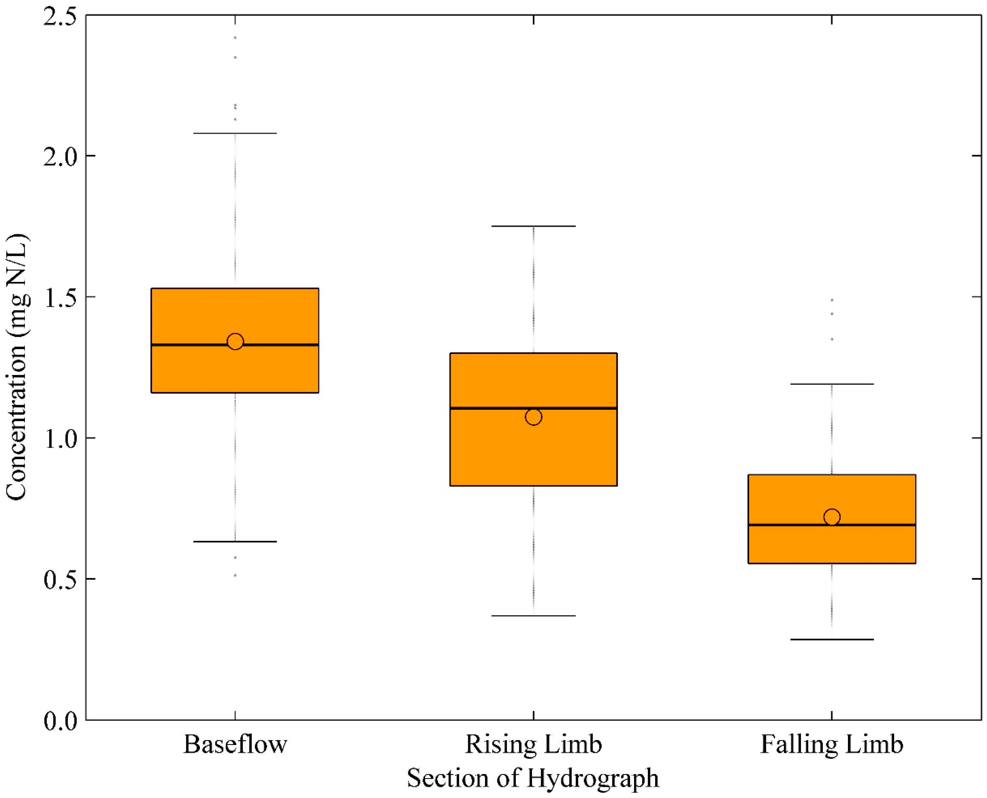
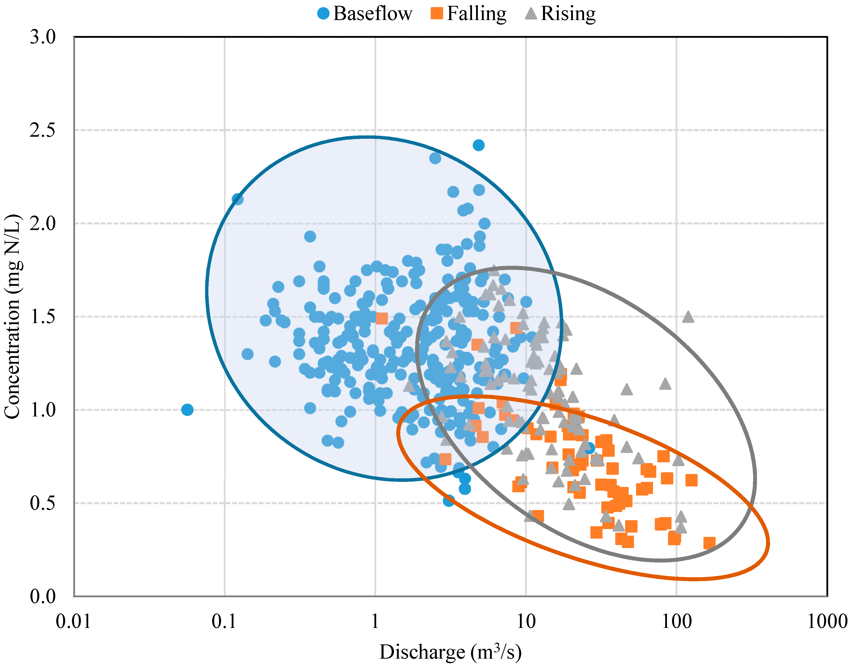
3.1. Analysis of Nitrate Grab Samples

Figure 4 shows boxplots for historic nitrate concentration samples (mg N/L) collected by USGS at different stages of the hydrograph (Baseflow, Rising, Falling). As displayed in the Figure 4, baseflow samples reflect higher concentrations compared with the other groups, and falling samples exhibit the lowest concentrations amongst all groups. The three group means differed significantly (p < 0.01) from each other. When the sample concentrations were plotted against discharge (Figure 5), a clear clustering pattern was observed. The difference between the rising and falling limb sample concentrations can be tied to hysteresis in the discharge-concentration relationship for any single event.

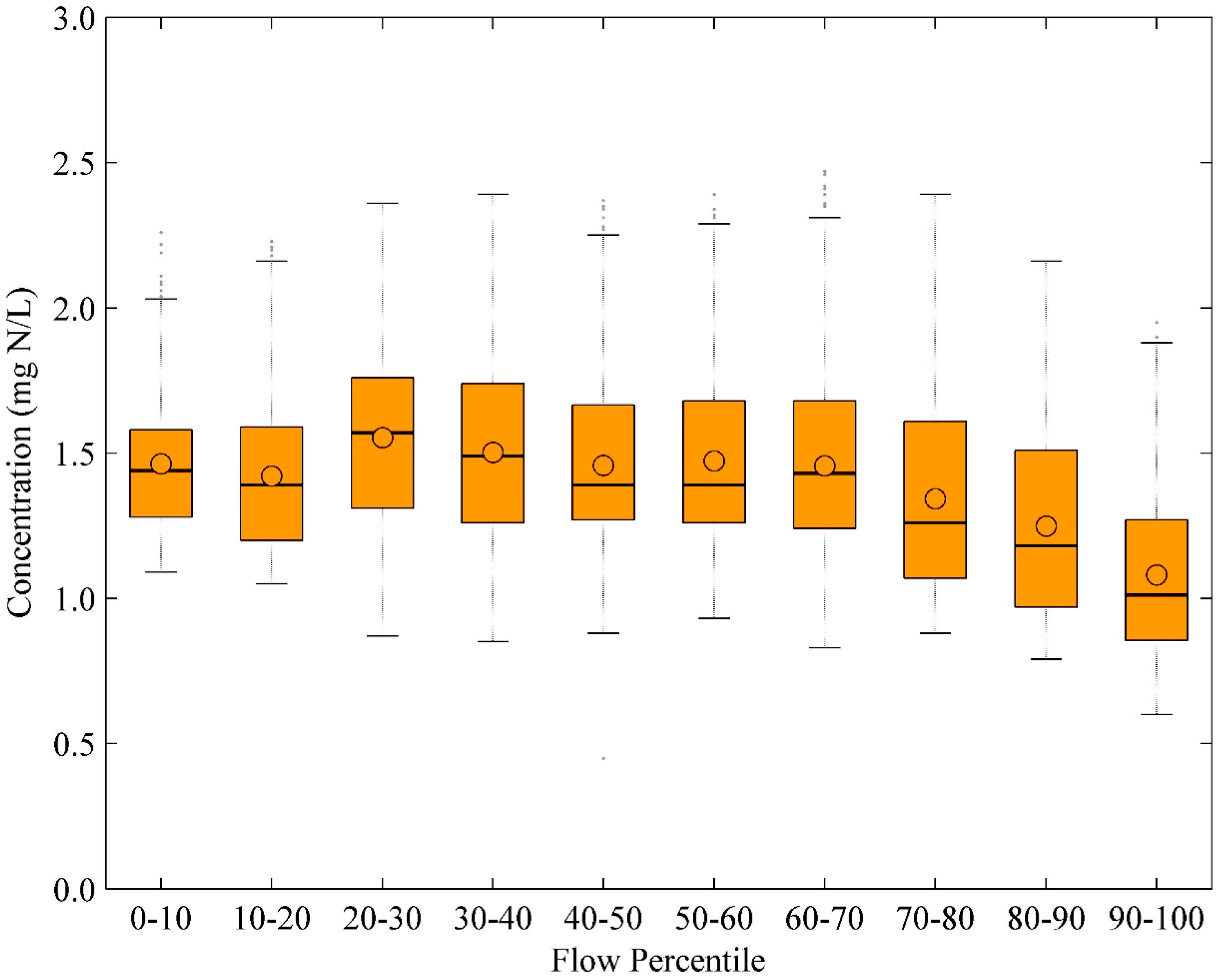
3.2. Analysis of Real-Time Nitrate Data

Time series of Thirty-four separate storm events of varying magnitudes were identified and isolated during the in-situ monitoring period within the Greensboro watershed. Likewise, time series of nitrate loadings were created for each storm event by using high resolution nitrate concentration data multiplied by USGS collected streams. Analysis of the nitrate loading time series revealed that during this monitoring period, 54% of the nitrate load was delivered through baseflow and 46% was through stormflow. Of the storm delivered nitrate loading, 45% was transported during the rising limb and the rest (55%) was through the falling limb of the storm. The maximum instantaneous nitrate loading rate during the monitoring period was ~4500 kg/day.

To test whether hysteresis has a strong role in nitrate delivery in the Greensboro watershed, concentrations for each event were plotted against discharge. Figure 6 plots results for five selected storm events (out of 34); the selected events cover the range of monitored storm magnitudes. All events exhibited a form of positive hysteresis effect (clockwise loop), whereby constituent concentrations on the rising limb of a storm hydrograph were higher than those measured at equivalent flows on the falling limb. Data in Figure 6 also demonstrate that the hysteresis loops all tend to fall from top-left to bottom-right, suggesting that there is a dilution of nitrate on the rising limb of each storm event, as discussed by [36].

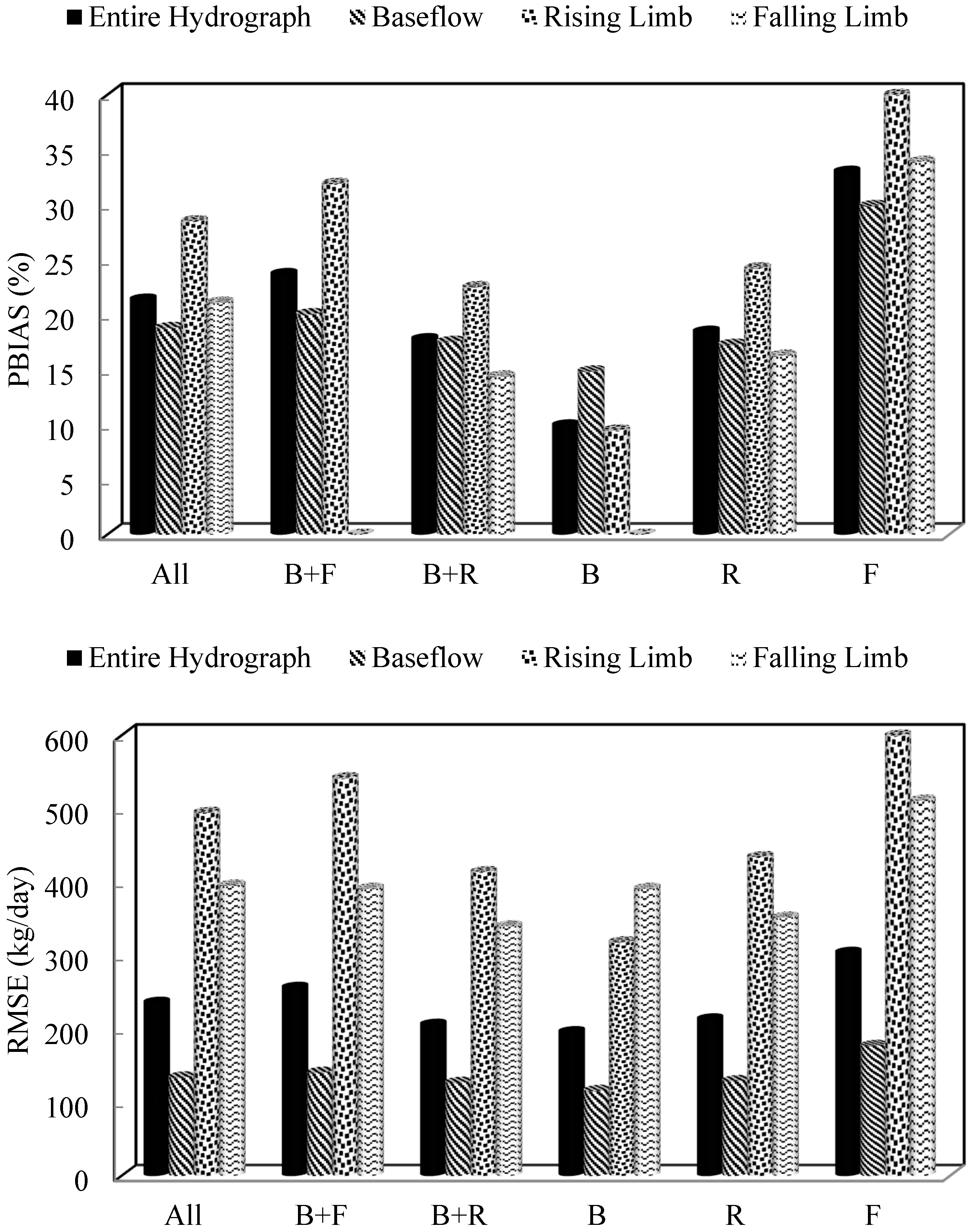
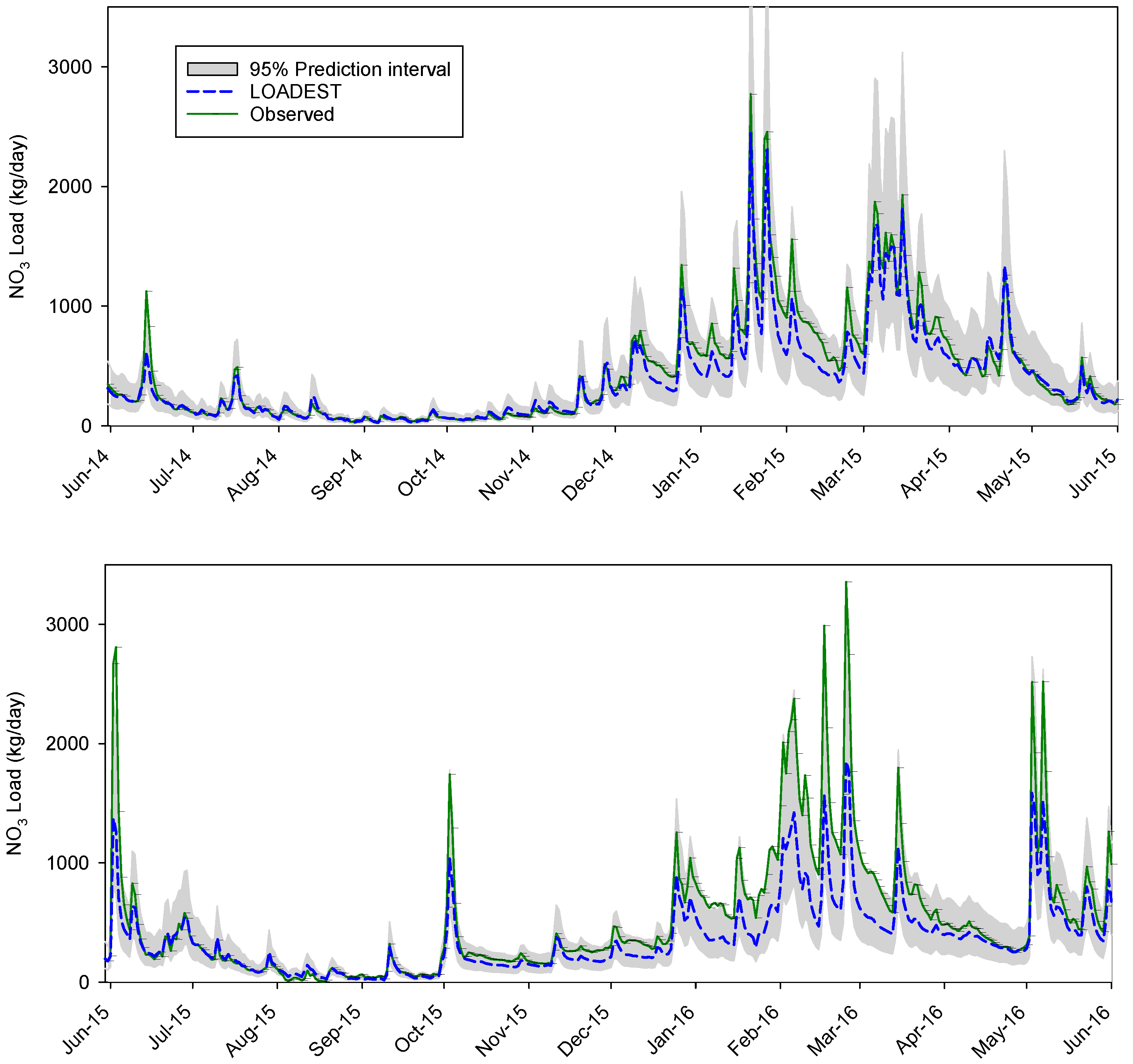
3.3. LOADEST Regression Analysis

LOADEST was conducted five times, using various groups of concentration databases described earlier (All, Rising (denoted with “R” model); Falling (denoted with “F” model); Base-Rising (denoted with “B + R” model); and Base-Falling (denoted with “B + F” model)), as well as the associated equivalent discharge rates at the time of sampling.

Table 1. Regression coefficients and goodness of fit for various calibration datasets from LOADEST.

Calibration Dataset	$\mathit{n}$	${\mathit{a}}_0$	${\mathit{a}}_1$	${\mathit{a}}_2$	${\mathit{R}}^2$	$\mathit{M}\mathit{S}\mathit{E}$
All	455	6.1043	0.8492	−0.0459	0.95	0.0766
Base + Rising	391	5.8298	0.9125	−0.0295	0.95	0.0669
Base + Falling	354	6.0002	0.8357	−0.0524	0.95	0.0684
Baseflow	291	5.0926	0.9765	−0.0006	0.94	0.0568
Rising	100	7.1893	0.8060	−0.0240 ₦	0.82	0.0929
Falling	63	7.0563	0.7218	−0.0313 ₦	0.85	0.0880

Notes: ^₦ Significant at p < 0.05 level. The rest of the parameters are significant at p < 0.01 level. n is sample size, MSE is mean square error of prediction (residual variance).

presents the LOADEST fitting results for each group. All the regression estimates in Table 1 are significant at a p < 0.05 level. As one might expect, the two regression models with the lowest number of samples (Rising, n = 100 and Falling, n = 63) have the smallest proportion of variation explained (0.82 < R² < 0.85) and more residual variance compared with the other regression models (R² > 0.94).

Based on the 95% prediction interval around regression model “All” (LOADEST model calibrated using all available USGS samples), as shown in Figure 3, the uncertainty bands grow larger around high flow conditions and become much narrower during low baseflow conditions. For the most part, the observed loading line is contained within (or close to the boundary) of the 95% prediction interval, except for one peak that occurs in June 2015.

3.4. Validation of Regression Analysis

The regression relationships were validated against observed (real-time sensor) loading data using the percent bias (PBIAS) and root mean square error (RMSE) of prediction. Note that PBIAS and RMSE of prediction were calculated for the whole real-time observation period (entire hydrograph) and at different stages of the hydrograph (i.e., baseflow, rising limb, and falling limb) (Figure 7). This assessment provides insight into what stages of the hydrograph are more uncertain and harder to predict.

As illustrated by the top panel of Figure 7, all models underestimate nitrate loading in almost all sections of the hydrograph (except for falling limb of B and B + F models). This can also be seen in Figure 3, where the observed time series exceeded the average loading prediction of the “All” regression model throughout most of the monitoring period. It is interesting to note that during some periods (e.g., from January 2016 to March 2016), the observed nitrate loading line falls close to the upper 95% prediction band of the regression model. The F model (model calibrated with only falling data) consistently showed higher errors (PBIAS and RMSE) compared with all other models, even when predicting falling conditions.

4. Discussion

4.1. Effect of Sampling Time on Storm Load Prediction

Judging by the PBIAS of predictions, the B model produced the most accurate predictions with the smallest PBIAS in all categories. However, considering the absolute error (as gauged by RMSE), the B model had comparable performance with R model for almost all validation categories. Note that B model had almost 3 times as many calibration samples as the R model (n = 291 vs. n = 100). The fact that R model, which was calibrated with only 100 (USGS) samples (n = 100), performed comparable to—or even better than—every other regression model at every validation category is an important finding. This finding supports our hypothesis that water quality samples collected over the whole range of flows/conditions do not always produce the most optimal regression model, as R model outperformed “All” model, which benefits from the most complete calibration dataset (n = 455).

The highest RMSE bars for each regression model with great consistency belong to validation during the rising limb of the hydrograph. This indicates that nitrate loads delivered through the rising limb are the most uncertain and hardest to predict. Looking at the lower panel of Figure 7, it could be said that all models predict baseflow conditions almost equally well. This suggests that if one’s interest is primarily in baseflow conditions, any calibration dataset would yield equally good prediction models.

Measurement uncertainty and its associated impact on model predictions (or other purposes) can be rarely found in the literature. It is stated by [37,38] that measurement uncertainty may be addressed by using various statistical approaches. However, the fundamental issue (concern) of measurement uncertainty cannot be properly resolved with insufficient data. In this study, nutrient data were measured on a daily temporal scale, which is the most detailed observation data available in the United States (and possibly around the world). Therefore, scientists and engineers can take advantage of the proposed work in more advanced applications in their future studies.

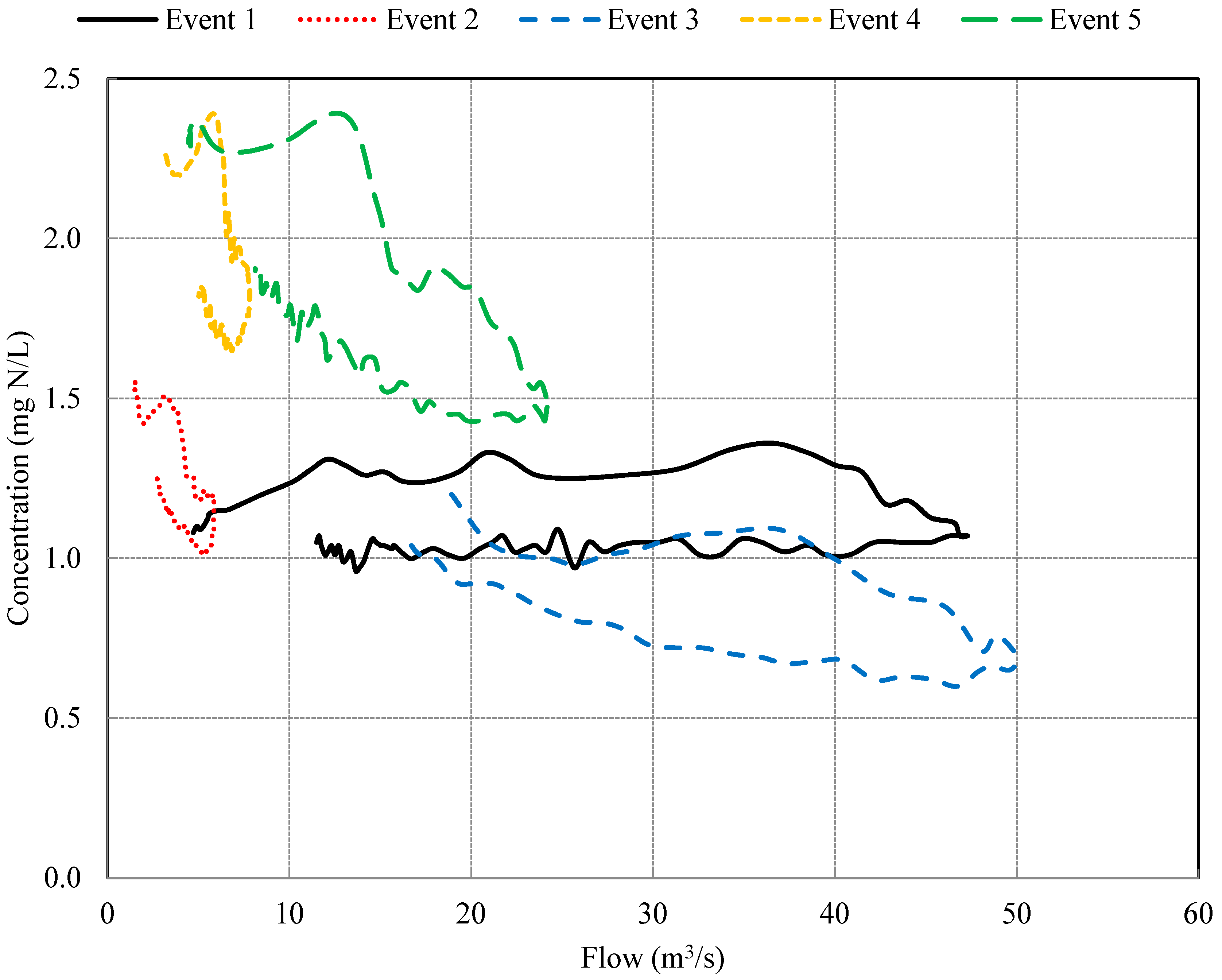
4.2. Effect of Hysteresis on Nitrate Load Estimation

The effect of storm events on nitrate loading may have different responses, depending on whether the watershed is a groundwater- or surface-dominated system and the availability and location of stored nitrate in the landscape [37,38,39]. In this study, one thing is clear: that changes in the hydrologic regime may affect the interactions between stream discharge and nitrate concentration, whereas the fate and transport of nitrate could also be affected consequently [40]. Previous studies have shown that small changes in year-to-year variations in antecedent soil moisture conditions may significantly affect the hydrochemistry in a watershed [40,41,42]. It has been reported [42] that nitrate concentration increases during storm events with dry antecedent conditions. As is evident from the positive hysteresis observed in this study (Figure 6), there is a dilution of nitrate on the rising limb of each storm event within the Greensboro watershed. Several researches have reported similar response for agricultural watersheds [43,44,45].

Figure 8 shows boxplots of storm nitrate concentration at different flow percentiles for all monitored storm events and demonstrates that median storm nitrate concentration decreases with increases in flow. The variation in storm nitrate concentration is more pronounced for midrange flows (30th–60th percentile) and less pronounced for low and high flows. Nitrogen loss is often computed as loads at the watershed outlet. Discharge at the watershed outlet is used by regression models such as LOADEST to estimate loads; in other words, nitrogen loss estimates are strongly influenced by discharge. However, due to the hysteresis effects, concentration becomes just as important during significant storm events so that loads cease to be predictable based on observed discharge.

4.3. Potential Impact on Correlated Applications

Effect of water-quality sampling techniques may have crucial impact on relevant studies in broader perspective. In recent years, water resources and environmental engineering subjects were mostly conducted by the approach of watershed modeling. Limited and valuable financial resources may be saved considerably, since the cost of trial-and-error approach via computers is a lot lower than actual implementations in the field. For example, the Conservation Effects Assessment Project (CEAP)–Wildlife was conducted by comparing nine financially applicable scenarios in the Western Lake Erie Basin [46,47,48]. Interactions between fish communities and nutrients (pollutants) were simulated and explored in sophisticated fashion. In addition, [49] validated current conditions of nutrients in the Great Lakes by comparing five independent watershed modeling projects [49]. Previous goals made in 1970s on nutrient reduction were examined with more advanced conservation scenarios and by using the latest technology. On the other hand, quality of measurement data used to conduct the corresponding projects was rarely examined in a proper manner [23]. It was stated in the literature that modeling results may be substantially altered by various sources of uncertainty such as model parameter, forcing inputs, operational structure, and measurement data [22,50]. Therefore, most of the currently available studies may require further investigation in the future.

5. Conclusions

In this study, the performance of the regression models was calibrated and evaluated by nitrate samples covering the entire range of the storm hydrograph versus the regression models, calibrated using a subset of the database covering specific hydrologic conditions. Throughout most of the monitoring period, the observed time series exceeded the average load predicted by all the regression models.

Considering the absolute error (as gauged by RMSE), the R model, which was calibrated with the lowest number of USGS samples, performed equally as well as or better than every other regression model at every validation category. The regression analysis tool, LOADEST, developed to conduct loadings estimation, does not account for changes in nitrate concentration at different stages of storm hydrographs, or for the nitrate hysteresis effect. In-situ measurement of nitrate in this study showed strong nitrate hysteresis with concentrations per unit flow higher in the rising limb than during the falling limb of storm hydrographs (clockwise). This resulted in loads estimated using nitrate concentrations measured on the rising limb to be higher than loads estimated from concentrations measured on the falling limb. Results derived in this study have indicated that nitrate loads delivered through the rising limb are the most uncertain source and may be difficult to be predict using regression models.

Given the complexity of hysteretic effects on water quality data, complex interactions among changing watershed conditions could lead to substantial nitrate flux uncertainty, based on periodic grab sample monitoring approaches. Therefore, in-situ sampling may be the most appropriate data source for estimating nitrate and other pollutant loadings affected by hysteresis effects. Scientists and engineers should take advantage of the proposed findings in future studies to enhance the quality of the associated decision making processes.

References

1. Granata, F.; Papirio, S.; Esposito, G.; Gargano, R.; de Marinis, G. Machine learning algorithms for the forecasting of wastewater quality indicators. Water 2017, 9, 105. [Google Scholar] [CrossRef]
2. Runkel, R.L.; Crawford, C.G.; Cohn, T.A. Load Estimator (Loadest): A Fortran Program. for Estimating Constituent Loads in Streams and Rivers; Science for the Changing World: Reston, VA, USA, 2004; Chapter A5. [Google Scholar]
3. Park, Y.; Engel, B.; Frankenberger, J.; Hwang, H. A web-based tool to estimate pollutant loading using loadest. Water 2015, 7, 4858–4868. [Google Scholar] [CrossRef]
4. Maier, H.; Dandy, G. The use of artificial neural networks for the prediction of water quality parameters. Water Resour. Res. 1996, 32, 1013–1022. [Google Scholar] [CrossRef]
5. Maier, H.; Dandy, G. Reply [to “Comment on ‘The use of artificial neural networks for the prediction of water quality parameters’ by H. R. Maier and G. C. Dandy”]. Water Resour. Res. 1997, 33, 2425–2427. [Google Scholar] [CrossRef]
6. Han, H.; Chen, Q.; Qiao, J. An efficient self-organizing rbf neural network for water quality prediction. Neural Netw. 2011, 24, 717–725. [Google Scholar] [CrossRef] [PubMed]
7. Partalas, I.; Tsoumakas, G.; Hatzikos, E.; Vlahavas, I. Greedy regression ensemble selection: Theory and an application to water quality prediction. Inf. Sci. 2008, 178, 3867–3879. [Google Scholar] [CrossRef]
8. Chen, Y.; Xu, J.; Yu, H.; Zhen, Z.; Li, D. Three-dimensional short-term prediction model of dissolved oxygen content based on pso-bpann algorithm coupled with kriging interpolation. Math. Probl. Eng. 2016, 2016. [Google Scholar] [CrossRef]
9. Xu, L.; Liu, S. Study of short-term water quality prediction model based on wavelet neural network. Math. Comput. Model. 2013, 58, 801–807. [Google Scholar] [CrossRef]
10. Cerro, I.; Antiguedad, I.; Srinavasan, R.; Sauvage, S.; Volk, M.; Sanchez-Perez, J. Simulating land management options to reduce nitrate pollution in an agricultural watershed dominated by an alluvial aquifer. J. Environ. Qual. 2014, 43, 67–74. [Google Scholar] [CrossRef] [PubMed]
11. Jha, M.; Gassman, P.; Arnold, J. Water quality modeling for the raccoon river watershed using swat. Trans. ASABE 2007, 50, 479–493. [Google Scholar] [CrossRef]
12. Duan, S.; Kaushal, S.S.; Groffman, P.M.; Band, L.E.; Belt, K.T. Phosphorus export across an urban to rural gradient in the chesapeake bay watershed. J. Geophys. Res. Biogeosci. 2012, 117. [Google Scholar] [CrossRef]
13. Brigham, M.E.; Wentz, D.A.; Aiken, G.R.; Krabbenhoft, D.P. Mercury cycling in stream ecosystems. 1. Water column chemistry and transport. Environ. Sci. Technol. 2009, 43, 2720–2725. [Google Scholar] [CrossRef] [PubMed]
14. Dornblaser, M.M.; Striegl, R.G. Suspended sediment and carbonate transport in the yukon river basin, alaska: Fluxes and potential future responses to climate change. Water Resour. Res. 2009, 45. [Google Scholar] [CrossRef]
15. Park, Y.S.; Engel, B.A. Use of pollutant load regression models with various sampling frequencies for annual load estimation. Water 2014, 6, 1685–1697. [Google Scholar] [CrossRef]
16. Walling, D.E.; Foster, I.D.L. Variations in natural chemical concentration of river water during flood flows, and lag effect—Some further comments. J. Hydrol. 1975, 26, 237–244. [Google Scholar] [CrossRef]
17. Evans, C.; Davies, T.D. Causes of concentration/discharge hysteresis and its potential as a tool for analysis of episode hydrochemistry. Water Resour. Res. 1998, 34, 129–137. [Google Scholar] [CrossRef]
18. House, W.A.; Warwick, M.S. Hysteresis of the solute concentration/discharge relationship in rivers during storms. Water Res. 1998, 32, 2279–2290. [Google Scholar] [CrossRef]
19. Beck, M. Water-quality modeling—A review of the analysis of uncertainty. Water Resour. Res. 1987, 23, 1393–1442. [Google Scholar] [CrossRef]
20. King, K.W.; Harmel, R.D. Comparison of time-based sampling strategies to determine nitrogen loading in plot-scale runoff. Trans. ASAE 2004, 47, 1457–1463. [Google Scholar] [CrossRef]
21. Meals, D.W.; Richards, R.P.; Dressing, S.A. Pollutant Load Estimation for Water Quality Monitoring Projects; Tech Notes 8; Developed for U.S. Environmental Protection Agency by Tetra Tech, Inc.: Fairfax, VA, USA, 2013; p. 21. [Google Scholar]
22. Yen, H.; Wang, X.; Fontane, D.; Harmel, R.; Arabi, M. A framework for propagation of uncertainty contributed by parameterization, input data, model structure, and calibration/validation data in watershed modeling. Environ. Model. Softw. 2014, 54, 211–221. [Google Scholar] [CrossRef]
23. Yen, H.; Hoque, Y.; Wang, X.; Harmel, R. Applications of explicitly incorporated/post-processing measurement uncertainty in watershed modeling. J. Am. Water Resour. Assoc. 2016, 52, 523–540. [Google Scholar] [CrossRef]
24. Pellerin, B.A.; Bergamaschi, B.A.; Gilliom, R.J.; Crawford, C.G.; Saraceno, J.; Frederick, C.P.; Downing, B.D.; Murphy, J.C. Mississippi river nitrate loads from high frequency sensor measurements and regression-based load estimation. Environ. Sci. Technol. 2014, 48, 12612–12619. [Google Scholar] [CrossRef] [PubMed]
25. Pellerin, B.A.; Saraceno, J.F.; Shanley, J.B.; Sebestyen, S.D.; Aiken, G.R.; Wollheim, W.M.; Bergamaschi, B.A. Taking the pulse of snowmelt: In-situ sensors reveal seasonal, event and diurnal patterns of nitrate and dissolved organic matter variability in an upland forest stream. Biogeochemistry 2012, 108, 183–198. [Google Scholar] [CrossRef]
26. Heffernan, J.B.; Cohen, M.J. Direct and indirect coupling of primary production and diel nitrate dynamics in a subtropical spring-fed river. Limnol. Oceanogr. 2010, 55, 677–688. [Google Scholar] [CrossRef] [Green Version]
27. Sprague, L.A.; Langland, M.; Yochum, S.; Edwards, R.; Blomquist, J.; Phillips, S.; Shenk, G.; Preston, S. Factors Affecting Nutrient Trends in Major Rivers of the Chesapeake bay Watershed; Water Resources Investigations Report 00-4218; U.S. Geological Survey: Richmond, VA, USA, 2000.
28. Ator, S.W.; Denver, J.M. Estimating contributions of nitrate and herbicides from groundwater to headwater streams, northern atlantsdic coastal plain, United States. J. Am. Water Resour. Assoc. 2012, 48, 1075–1090. [Google Scholar] [CrossRef]
29. McCarty, G.W.; McConnell, L.L.; Hapernan, C.J.; Sadeghi, A.; Graff, C.; Hively, W.D.; Lang, M.W.; Fisher, T.R.; Jordan, T.; Rice, C.P.; et al. Water quality and conservation practice effects in the choptank river watershed. J. Soil Water Conserv. 2008, 63, 461–474. [Google Scholar] [CrossRef]
30. McCarty, G.W.; Hapeman, C.J.; Rice, C.P.; Hively, W.D.; McConnell, L.L.; Sadeghi, A.M.; Lang, M.W.; Whitall, D.R.; Bialek, K.; Downey, P. Metolachlor metabolite (MESA) reveals agricultural nitrate-n fate and transport in choptank river watershed. Sci. Total Environ. 2014, 473, 473–482. [Google Scholar] [CrossRef] [PubMed]
31. Lim, K.J.; Engel, B.A.; Tang, Z.X.; Choi, J.; Kim, K.S.; Muthukrishnan, S.; Tripathy, D. Automated web gis based hydrograph analysis tool, what. J. Am. Water Resour. Assoc. 2005, 41, 1407–1416. [Google Scholar] [CrossRef]
32. Evaldi, R.D.; Moore, B.L. Techniques for Estimating the Quantity and Quality of Storm Runoff from Urban Watersheds of Jefferson County, Kentucky; Water-Resources Investigations Report 94-4023; U.S. Geological Survey: Louisville, KY, USA, 1994.
33. Cohn, T.A.; Gilroy, E.J.; Baier, W.G. Estimating Fluvial Transport of Trace Constituents Using a Regression Model with Data Subject to Censoring; U.S. Geological Survey: Reston, VA, USA, 1992.
34. Kutner, M.H.; Nachtsheim, C.; Neter, J.; Li, W. Applied Linear Statistical Models, 5th ed.; McGraw-Hill/Irwin: New York, NY, USA, 2005; pp. 214–247. ISBN 0-07-238688-6. [Google Scholar]
35. Gupta, H.V.; Sorooshian, S.; Yapo, P.O. Status of automatic calibration for hydrologic models: Comparison with multilevel expert calibration. J. Hydrol. Eng. 1999, 4, 135–143. [Google Scholar] [CrossRef]
36. Lloyd, C.; Freer, J.; Johnes, P.; Collins, A. Using hysteresis analysis of high-resolution water quality monitoring data, including uncertainty, to infer controls on nutrient and sediment transfer in catchments. Sci. Total Environ. 2016, 543, 388–404. [Google Scholar] [CrossRef] [PubMed]
37. Webb, B.W.; Walling, D.E. Nitrate behavior in streamflow from a grassland catchment in Devon, UK. Water Res. 1985, 19, 1005–1016. [Google Scholar] [CrossRef]
38. Yates, C.; Johnes, P. Nitrogen speciation and phosphorus fractionation dynamics in a lowland chalk catchment. Sci. Total Environ. 2013, 444, 466–479. [Google Scholar] [CrossRef] [PubMed]
39. Chen, N.; Wu, J.; Hong, H. Effect of storm events on riverine nitrogen dynamics in a subtropical watershed, southeastern china. Sci. Total Environ. 2012, 431, 357–365. [Google Scholar] [CrossRef] [PubMed]
40. Davis, C.A.; Ward, A.S.; Burgin, A.J.; Loecke, T.D.; Riveros-Iregui, D.A.; Schnoebelen, D.J.; Just, C.L.; Thomas, S.A.; Weber, L.J.; St Clair, M.A. Antecedent moisture controls on stream nitrate flux in an agricultural watershed. J. Environ. Qual. 2014, 43, 1494–1503. [Google Scholar] [CrossRef] [PubMed]
41. Macrae, M.; English, M.; Schiff, S.; Stone, M. Influence of antecedent hydrologic conditions on patterns of hydrochemical export from a first-order agricultural watershed in Southern Ontario, Canada. J. Hydrol. 2010, 389, 101–110. [Google Scholar] [CrossRef]
42. Biron, P.; Roy, A.; Courschesne, F.; Hendershot, W.; Cote, B.; Fyles, J. The effects of antecedent moisture conditions on the relationship of hydrology to hydrochemistry in a small forested watershed. Hydrol. Process. 1999, 13, 1541–1555. [Google Scholar] [CrossRef]
43. Lloyd, C.E.M.; Freer, J.E.; Johnes, P.J.; Collins, A.L. Technical Note: Testing an improved index for analysing storm discharge-concentration hysteresis. Hydrol. Earth Syst. Sci. 2016, 20, 625–632. [Google Scholar] [CrossRef]
44. Bowes, M.J.; Jarvie, H.P.; Halliday, S.J.; Skeffington, R.A.; Wade, A.J.; Loewenthal, M.; Gozzard, E.; Newman, J.R.; Palmer-Felgate, E.J. Characterising phosphorus and nitrate inputs to a rural river using high-frequency concentration-flow relationships. Sci. Total Environ. 2015, 511, 608–620. [Google Scholar] [CrossRef] [PubMed] [Green Version]
45. Ferrant, S.; Laplanche, C.; Durbe, G.; Probst, A.; Dugast, P.; Durand, P.; Sanchez-Perez, J.M.; Probst, J.L. Continuous measurement of nitrate concentration in a highly event-responsive agricultural catchment in south-west of france: Is the gain of information useful? Hydrol. Process. 2013, 27, 1751–1763. [Google Scholar] [CrossRef] [Green Version]
46. Daggupati, P.; Yen, H.; White, M.; Srinivasan, R.; Arnold, J.; Keitzer, C.; Sowa, S. Impact of model development, calibration and validation decisions on hydrological simulations in west lake erie basin. Hydrol. Process. 2015, 29, 5307–5320. [Google Scholar] [CrossRef]
47. Keitzer, S.; Ludsin, S.; Sowa, S.; Annis, G.; Arnold, J.; Daggupati, P.; Froehlich, A.; Herbert, M.; Johnson, M.; Sasson, A.; et al. Thinking outside of the lake: Can controls on nutrient inputs into lake erie benefit stream conservation in its watershed? J. Great Lakes Res. 2016, 42, 1322–1331. [Google Scholar] [CrossRef]
48. Yen, H.; White, M.; Arnold, J.; Keitzer, S.; Johnson, M.; Atwood, J.; Daggupati, P.; Herbert, M.; Sowa, S.; Ludsin, S.; et al. Western lake erie basin: Soft-data-constrained, nhdpius resolution watershed modeling and exploration of applicable conservation scenarios. Sci. Total Environ. 2016, 569, 1265–1281. [Google Scholar] [CrossRef] [PubMed]
49. Scavia, D.; Kalcic, M.; Muenich, R.; Read, J.; Aloysius, N.; Bertani, I.; Boles, C.; Confesor, R.; DePinto, J.; Gildow, M.; et al. Multiple models guide strategies for agricultural nutrient reductions. Front. Ecol. Environ. 2017, 15, 126–132. [Google Scholar] [CrossRef]
50. Ajami, N.; Duan, Q.; Sorooshian, S. An integrated hydrologic bayesian multimodel combination framework: Confronting input, parameter, and model structural uncertainty in hydrologic prediction. Water Resour. Res. 2007, 43. [Google Scholar] [CrossRef]
Figure 1. The location of the Greensboro watershed within the Choptank River basin.
Water 09 00895 g001
Figure 2. A graph used to verify the stability of the global nitrate calibration used with the in-situ sensor. The red points are from dilution of natural water containing nitrate, and the black points are from standard addition of known nitrate amount to the natural water.
Water 09 00895 g002
Figure 3. Time series of real-time-monitored nitrate loading at the outlet of the Greensboro watershed, compared with the LOAD ESTimator (LOADEST) regression relationship and its respected 95% prediction interval. The LOADEST model was calibrated using all available USGS samples (All).
Water 09 00895 g003
Figure 4. Box plot of USGS samples of nitrate concentration during various sections of the hydrograph. The error bars and circles inside the colored boxes represent the median and mean of the data. The lower and upper edges of boxes represent 25th and 75th percentiles. The error bars outside the colored boxes represent the 10th and 90th percentiles, and the dots represent 5th and 95th percentiles.
Water 09 00895 g004
Figure 5. Clustering of various USGS-collected nitrate sample groups. Note that horizontal axis is plotted in logarithmic scale. The ellipses are drawn to visually identify clustering of samples. (m3/s).
Water 09 00895 g005
Figure 6. Hysteresis effect observed for five individual events of varying magnitude during the real-time monitoring period. (m3/s).
Water 09 00895 g006
Figure 7. Validation of LOADEST regression models at different stages of the hydrograph. On the x axis, “All” represents the regression model built by using all USGS grab samples. Subsequently B, R, and F denote “Baseflow”, “Rising”, and “Falling” models. B + F and B + R denote “Baseflow + Rising” and “Baseflow + Falling” models.
Water 09 00895 g007
Figure 8. Boxplots of storm nitrate concentration at different flow percentiles for all monitored storm events. The error bars and circles inside the colored boxes represent the median and mean of the data. The lower and upper edges of boxes represent 25th and 75th percentiles. The error bars outside the colored boxes represent the 10th and 90th percentiles, and the dots represent 5th and 95th percentiles.
Water 09 00895 g008