Optimal Allocation Method of Irrigation Water from River and Lake by Considering the Field Water Cycle Process


1
Center for Agricultural Water Research in China, China Agricultural University, Beijing 100083, China
2
Institute of Water Resources for Pastoral Area, Ministry of Water Resources of China, Huhhot 010018, China
*
Author to whom correspondence should be addressed.
Water 2017, 9(12), 911; https://doi.org/10.3390/w9120911
Submission received: 29 September 2017
/
Revised: 20 November 2017
/
Accepted: 20 November 2017
/
Published: 23 November 2017
(This article belongs to the Special Issue Advances in Agriculture Water Efficiency)
Abstract
:At present, the shortage of water resources has become a serious constraint to the further development of social economy. The optimal allocation of multi-water resources is valuable for agricultural water management in arid and semi-arid regions. However, traditional deterministic programming does not solve the complex water resources allocation in irrigation systems. Furthermore, previous allocation methods of irrigation water seldom considered the water cycle process, especially for multi-sources of irrigation. In this study, we develop an inexact fuzzy stochastic simulation-optimization programming (IFSSOP) model for the irrigation water optimal allocation of two water sources. The model combines the crop water model and the field water cycle model with an uncertainty optimization model, which considers the contribution of groundwater to crop water consumption. As a case study, the developed model is used in an arid area with two irrigation water sources: a river and a lake. Accordingly, the total optimal allocation irrigation water amounts of river and lake water under different violation probabilities in various hydrological years were obtained. By comparing the IFSSOP model with the IFSSOP model without considering the contribution of shallow groundwater (IFSSOP-NG model), it can be shown that the system benefits of the developed model are higher. With the lake water source from flood water, the region can save 30–34% of the river water, maintaining the original crop water deficit irrigation ratio. Consequently, application of the IFSSOP model in irrigation scheduling will provide effective water allocation patterns to save more water in an arid region with shallow groundwater.
1. Introduction
Water scarcity is a major factor constraining agricultural development in many arid and semi-arid areas of the world. Generally, the limited water resources will not be able to meet the increasing irrigation water requirements. Thus, any measures to improve water use efficiency are useful to food production [1,2]. Furthermore, improving irrigation scheduling is one of the most effective ways of increasing irrigation efficiency to cope with the shortage of water resources [3].
One of the most important problems is how to allocate the irrigation water in the different growing stages of crops to get the highest yield and benefit under water shortages. This requires the determination of an optimum irrigation schedule under limited irrigation water supply. Some system methods, including dynamic programming (DP), linear programming (LP), and nonlinear programming (NLP), are the optimization approaches for irrigation scheduling. Furthermore, DP and NLP are most widely used [4,5,6,7]. Shangguan et al. [8] presented a recurrence control model for the regional optimal allocation of irrigation water resources that consists of three levels (layers), in which the first level involves dynamic programming (DP) to allocate water in different growth stages of a crop. Ghahraman and Sepaskhah [9] explored a nonlinear programming (NLP) optimization model with an integrated soil water balance performing over different crop growth stages that is able to handle integrated constraints in the optimization of irrigation water allocation; and this model enhanced the previous simple NLP model with no inclusion of soil water balance. An agricultural water resource system is in relation to various uncertain and complex variables, such as soil condition, water availability, market situation, and climate [10,11]. However, previous programming had difficulties addressing the uncertainty of the irrigation water optimal allocation process.
In response to this question, the application of new optimization techniques and uncertainty theory methods were proposed for optimizing water resources allocation [12,13,14,15,16,17]. Interval-parameter programming (IPP), fuzzy mathematical programming (FMP), and stochastic mathematical programming (SMP) were proposed for planning water resource systems. Recent studies have focused on developing an approach through integrating different programming into a general framework applied to crop planning and water resources allocation on a regional scale. For example, Maqsood et al. [18] developed an interval-parameter two-stage optimization model and applied it to allocate water from a reservoir to three farms cropped with alfalfa, wheat, and potato. Han et al. [19] developed an interval-parameter linear optimization model with stochastic vertices, which was applied to the optimization of Yellow River water for different crops, and the results indicated that water could be allocated to crops under different scenarios of water transfer. However, in many previous irrigation optimization models, only one water resource was considered, which cannot satisfy the irrigation requirements of local crops. The conjunctive use of multi-water resources is necessary to ensure the food productivity of irrigated districts [20,21,22]. The optimal allocation of multi-water resources based on the uncertainty theory method was proposed for supporting the irrigation system [23,24]. Shi et al. [25] proposed a fuzzy inexact two-phase programming, implying that more groundwater than surface water would be consumed for regional water resources allocation. In the same year, Guo et al. [26] introduced an interval-parameter to the Jensen model for agricultural water resource management. This model can obtain the optimal interval solutions of irrigation water (surface water and groundwater) for each crop during its various growth stages in three typical hydrological years. While Li et al. [15] considered more uncertainty variables and combined more methods to develop an inexact chance constrained semi-infinite mixed-integer multi-objective programming (ICSIMP) model for optimizing irrigation water resources allocation plans. These optimization models were useful for planning agriculture water resources allocation. However, most previous methods ignored crop responses to soil water at different stages and the agro-hydrological cycle. Furthermore, the process of crop water requirements, the dynamics of the soil moisture depletion process, and the water cycle in irrigation systems have not been discussed in detail, resulting in optimal allocation of water resources one-sidedly and passively.
After taking account of these, the objective of this paper is to develop an optimization model coupling crop water consumption and water conversion physical processes. The developed model can be used to allocate limited irrigation water resources for a crop in growth stages under multiple uncertainties. Furthermore, the correlativity between agriculture water saving potential and economic benefit is analyzed. A kind of water transform is proposed to introduce the saved irrigation water into the water markets and realize its greater economic value.
2. Study Area
2.1. Description of the Study Area
The Hetao irrigation district (HID) located along the Yellow River in Inner Mongolia, northern China, is one of the three largest irrigation districts in China (Figure 1). The HID covers an area of 1.12 Mha, and is mostly (570,000 ha) cultivated land. The region is a typical arid and semi-arid area, with annual precipitation of 160 mm and evaporation of 2240 mm [27]. The soil mainly consists of sandy loam [28]. The groundwater is shallow, with a depth varying from 1.2 to 3.8 m during the year [29]. Water scarcity is severe, with an annual diverted water volume from the Yellow River of approximately 5 billion m3. However, the Yellow River Water Conservancy Commission plans to reduce water diversion with water-saving projects. The Yellow River enters a freezing period in winter and breaks up in March of the following year with a large number of ice floods hazard downstream. Furthermore, special geological structures formed the unique phenomenon of lake enrichment in the HID, and lake water resources have a large potential for development and utilization. Under such circumstances, ice floods can be transferred to lakes so that farmers can irrigate fields with water brought from nearby lakes under irrigation water shortages. This can not only relieve the pressure of ice floods from the Yellow River but can also effectively improve water use efficiency.
In this study, Wangyedi Lake (WYDL), a typical lake, was selected as the case study. WYDL is located in west of the Hetao irrigation district and is close to the Wulanbuhe Desert. There are 100 ha of farmland around the lake, and maize is the main crop. Traditionally, the field is fed with Yellow River (YR) water. Drought often exists because of the shortage of irrigation water. Therefore, the ice floods are considered as a possible irrigation water resource. The lake water quality is consistent with the irrigation requirements. As a result, the lake can be used as the reserve for the ice floods. The field area, approximately 3 km away from the lake, is thought of as a valuable irrigation field using lake water. There is approximately 1 km of wasteland between the farmland and lake at the high groundwater level.
2.2. Data Collection
During the growing period, the meteorological data, consisting of air temperature, sunshine hours, daily rainfall, and other meteorological parameters from 1961 to 2010, were collected from the Linhe meteorological station close to WYDL. The empirical frequency method was used to calculate the typical hydrological years over 51 years, and the corresponding frequencies of the three typical years were 25%, 50%, 75%. By calculation, 1973, 1987, and 1982 were selected as the hydrological years, corresponding to a wet year, a normal year, and a dry year, respectively. The target of the developed model is to make total economic benefits maximization in different hydrological years. The price of maize, planting costs, irrigation water price, and water diverting costs need to be determined for the irrigation water resource optimization. The mean value does not fully reflect the actual situation, so fuzzy number was used to indicate the prices of maize products. The prices of maize products and the planting costs were derived from statistical data of the China Agricultural Product Price Information Network, and they are [1.8, 2.1, 2.4] Yuan kg−1, and 10,500 Yuan ha−1, respectively. For the water price, the agricultural water price is determined by the times according to the regulation plan, and from 11 April to 30 September, agricultural irrigation water is 0.083 Yuan m−3. Irrigation water resources from ice floods were not accounted for as adequate ice flood resources. However, a channel needs to be constructed to divert ice flood water to the lake, and the construction costs of the channel are considered in the model. In this study, the lake irrigation cost is 0.03 Yuan m−3 after investigation.
3. Methodology
Irrigation water resource allocation is determined by field hydrological processes, especially fluxes between groundwater in farmlands and soil water, and lake water. For crop water consumption, the impacts of soil water stress need to be considered. Additionally, there are some uncertainty factors, such as the uncertainties in diverted water volume, economic parameters, and reservoir capacity, as well as climate change. As a result, the inexact fuzzy stochastic simulation-optimization programming (IFSSOP) model is developed to allocate the limited irrigation water resources and ice flood resources. The IFSSOP model couples the hydrological cycle simulation model and uncertainty optimization model. Figure 2 indicates the general framework of the IFSSOP model. The four modules of the IFSSOP model consist of the water balance model, an actual evapotranspiration model, the Jensen model, and an optimization model of irrigation water allocation. The water balance model is used to describe the hydrological cycle. The crop yield can be the output with the Jensen model, in which actual evapotranspiration (ET) is the input. Furthermore, the ET model states that daily ET is impacted by soil water, which is a result of the hydrological model. The model takes a day as the basic time step, and a month as the growth stage. Overall, the decision variable (irrigation amount) of the optimization model is the input of the simulation model, and the objective variable is determined by the crop yield, which is the output of the simulation model.
3.1. The Hydrological Cycle Simulation Model
3.1.1. Water Balance Model
The field water balance considers the main components, i.e., irrigation (IW), precipitation (P), groundwater evaporation (ETg), irrigation infiltration (Dinf), and actual evapotranspiration (ET). Surface runoff was ignored because of low rainfall and relatively flat topography in the study region. In past, there were few irrigation schedule optimization models considering the effect of soil water deficit on crop evapotranspiration. The time step for field water balance is one day. The soil water balance equation for crops can be expressed as:
where i is a different day, namely, i = 1, 2, 3…; t is a different growth stage, including April, May, June, July, August, September, namely, t = 1, 2, 3…, and the total number of growth stages of crop T = 6; j is the type of the multi-water resources in the area, 1 and 2 stand for the Yellow River and lake water, respectively; ΔWi is the variation of water storage under 1 m depth soil in day i (mm); z is the depth of the soil, here z = 1 m; θi is the volumetric water content in day i (m3 m−3); A is the irrigation area(m2), A = 1,000,000 m2; η is the utilization coefficient of the water supply in the Hetao irrigation area; the efficiency coefficient of irrigation is 0.4; the efficiency coefficient of a sublateral canal is 0.9; and Qjt is the water amount of water resource j in growth stage t (m3). The groundwater recharge coefficients were 0.15, the irrigation water for I, and then the recharge of irrigation water to groundwater is Dinf = 0.15I [30].
Groundwater evaporation is an important way to transfer shallow groundwater to soil water and atmospheric water, and is also the main consumption of groundwater. Hu et al. [31] presented the empirical formula for calculating the groundwater evaporation, and the models were applied in Xinjiang with a high accuracy:
where E is the pan evaporation rate (mm), E = ET0/0.53 [32]; and h is phreatic depth (m). Phreatic depths during crop growth were calculated by the groundwater balance Equation (3) for each day.
For the HID, with shallow groundwater, the exchanges of groundwater with soil water and lake water are very strong. Groundwater recharge comes from field leakage; and groundwater consumption includes field phreatic evaporation and lateral discharge. On the basis of water balance, the relation between groundwater supply and demand can be studied:
where µ is the specific saturated soil water content (70 mm/m) for the Hetao irrigation area [33], R is the exchange capacity of groundwater and lake water (m3), and GA is the surface area that contributes to flow (m2). The paper sets the discharge of groundwater as the positive direction. The groundwater depth in the region floats approximately 1 m in late April; therefore, the initial value was set as h1 = 1 m. According to Darcy’s law, the exchange capacity of groundwater and lake water is described by the following equation:
where K is the horizontal hydraulic conductivity calculated by the water pumping experiment, K = 6.48 m/d; J is the horizontal hydraulic gradient, Ji = ΔHi/L; ΔHi is the difference of groundwater and lake water levels on day i; L is the length of the cross section; and A is the cross-sectional area of the aquifer, A = 4000 m2.
The irrigation amount extracted from the lake is constrained by the lake storage capacity. Lake water changes significantly due to strong evaporation; in other words, the amount of lake water varies with the climate. The lake’s main recharge comes from ice floods, precipitation, and the exchange capacity between the lake and groundwater. Thus, ice floods were drawn into the lake only during the thawing period. The output components consist of evaporation and irrigation. In particular, the relationship between recharge and discharge of lake and groundwater is dynamic rather than unilateral. Groundwater recharges the lake when the groundwater level exceeds the lake level. The lake water balance model was used to analyze the characteristics and causes of water changes.
where G is the ice flood (104 m3); V is the lake water storage capacity (104 m3); LA is the lake surface area (104 m2); LH is the lake water level (m); E0 is evaporation from the lake (mm), E0 = 0.55E [34]; and Q2i is the irrigation from the lake (m3).
3.1.2. Actual Evapotranspiration Model
Crop evapotranspiration depends on the potential evaporation (by reference crop evapotranspiration ET0), crop types and growth (by crop coefficient Kcb and the soil evaporation coefficient Ke), soil water supply (by soil water stress coefficient Ks), and the evapotranspiration is calculated by using the dual Kc approach [35]:
where ET0 is associated with meteorological factors and calculated in accordance with the FAO-56 recommended Penman-Monteith formula; the crop coefficients Kcb and Ke were determined with the meteorological data from the reference FAO-56; θfc is the volumetric water content at field capacity; θwp is the volumetric water content at wilting point; θt is the volumetric water content at the critical point of water stress, and the measured θfc, θwp, θt were used to calculate soil water stress coefficient Ks: θfc = 0.20, θwp = 0.08, θt = 0.14; and θ1 as initial value equal to θt.
3.1.3. Jensen Model
To reflect the sensitivity of crop yield affected by water deficit, the Jensen model is used to describe the relationship between crop yield and water requirement. The Jensen model is expressed as follows:
where Y is the actual yield of a crop (kg ha−1); Ym is the adequate maximum yield of a crop when the water supply is adequate (kg ha−1); ET is the actual evapotranspiration in the crop growth stage t (mm); ETm is the maximum evapotranspiration in the crop growth stage t (mm); and λt is the water sensitivity index in the crop growth stage t. Among them, according to the relevant experiment in the HID, the maximum yield of maize is 12,850 kg ha−1.
Usually, the Jensen model is used to calculate crop yield with the ET of a growth stage. Generally, the water sensitivity index in different growth stages was obtained from field experiments. In the study, a month is the stage of the model; therefore, the water sensitivity index of the growth stages needs to return, and it can solve the above problems by establishing the water sensitivity index [36]:
where t is the number of days after seeding. By the cumulative function Z(t), the water sensitivity index from ti−1 to ti can be calculated by the formula:
Wang [37] described the change in the cumulative value of the water sensitivity index over time by the logistic curve:
where K, b and m are empirical parameters.
The sensitivity index in the Jensen model was recalculated according to the month phase, the monthly ETm and λ of maize in the new model in Table 1.
3.2. Uncertainty Optimization Model of Irrigation Schedule with Multi-Water Resources
Between different hydrological years, evapotranspiration is an uncertain variable due to various climate conditions [38]. We adopted the 90% confidence interval value to express evapotranspiration ranges in various hydrological years [39]. Fuzzy programming can effectively reflect ambiguity and vagueness [40,41]. The price of maize, which is affected by the factors of society development and the benefit of water supply, is represented by fuzzy numbers. The IFSSOP model could be formulated as follows:
Objective:
where F± is the system net benefit in the study region (Yuan, Chinese monetary currency, 1 US $ ≈ 6.625 Yuan under the present exchange rate); CP is the price of a crop (Yuan kg−1); TC is the cost of a crop (Yuan ha−1); A is the area of planting of a crop (ha); and Sj is the cost of water coming from water resource j (Yuan m−3).
Constraints should be set in the optimization model of irrigation schedule with multi-water resources.
(1) The actual crop evapotranspiration constraints
The actual crop evapotranspiration of each time period should not exceed ETm.
(2) Water supply capacity from Yellow River constraints
The water supply of the Yellow River within a crop growth period as a rigid indicator of water can be used in irrigation, but no more than the maximum water supply QY can be used. The study area is fed by the Yellow River, approximately 69.2 thousand m3 at crop growth stages yearly.
(3) Lake ecological capacity constraints
The lake water storage in any period should not exceed the max capacity Vmax (three hundred and fifty thousand m3). Lake water storage capacity is more than the lake effective capacity B for ecological sustainable development, but more lake water is often divided for greater benefits in the actual making-decision process, allowing the existence of appropriate risk p. The stochastic chance-constrained programming can effectively reflect the reliability of the system to meet the constraints (or risk) [42]. The model can effectively solve uncertainties, described as intervals and fuzzy characteristics, which exist in the water resources allocation process. However, in many cases, policy makers want to understand different decision plans under different violation probabilities of lake water. Therefore, compared with the IFSOP model, the main advantage of the IFSSOP model is that it provides enough attention on the lake ecological constraints under violation probabilities.
where Pr denotes the probability of a random event; and the cumulative distribution function of B and the violation probabilities are given.
(4) The amount of water should be positive
4. Results and Discussion
4.1. Evaluation of the Inexact Fuzzy Stochastic Simulation-Optimization Programming (IFSSOP) Model
4.1.1. Water Amount Allocation under Different P in Different Hydrological Years
Figure 3 shows the total optimal irrigation water allocation of two water resources under various p in a wet year, normal year, and dry year, respectively. p = 0, 0.05, 0.1, and 0.2, representing the different risk levels of lake ecological constraint violations. The levels of p signify that the constraint would be satisfied with a probability of at least 95%, 90%, and 80%. Higher violating probabilities mean higher lake water availability. Figure 3 shows the explicit conclusion that the total irrigation water allocated to maize is pretty much the same in the three hydrological years. As the probability of risk increases, more and more water would be allocated to maize in the upper bound and the lower bound of three hydrological years. However, the phenomenon does not exist in the lower bound of a wet year because the crop water requirement was relatively low at the lower bound and there is enough water for irrigation in this circumstance. Therefore, YR water with a high cost was saved. In summary, maize can be fully irrigated with a lower crop water requirement and adequate water supply. This can save YR water amount of at least 22,000 m3 for the study district, and under a certain circumstance, more YR water will be saved with the increase of violation probabilities. The main irrigation water in the area is the Yellow River, and this is in accord with the actual situation, with lake water by using flood water, which belongs to extra water. Therefore, to achieve the effect of the Yellow River savings without reducing crop yield, some measures should be taken to use more flood water, such as excavation of artificial lakes for water storage.
4.1.2. System Economic Benefit under Different P in Different Hydrological Years
The maximum system economic benefit in different hydrological years at different violation probabilities is shown in Figure 4. As violation probabilities decrease, the system benefit would be decreased, which indicates that a lower p leads to a narrower decision space with higher reliability and lower system benefits. Combined with Figure 3, water supply, risk, and economic benefits have a positive correlation under water shortage. The policy makers should select the upper bound of irrigation water allocation to achieve a higher system economic benefit though it undertakes a larger risk. It is not the case under full irrigation, where the lower bound of water allocation obtained high system benefits in the wet year.
4.1.3. Water Consumption of Maize in Different Months of Different Hydrological Years
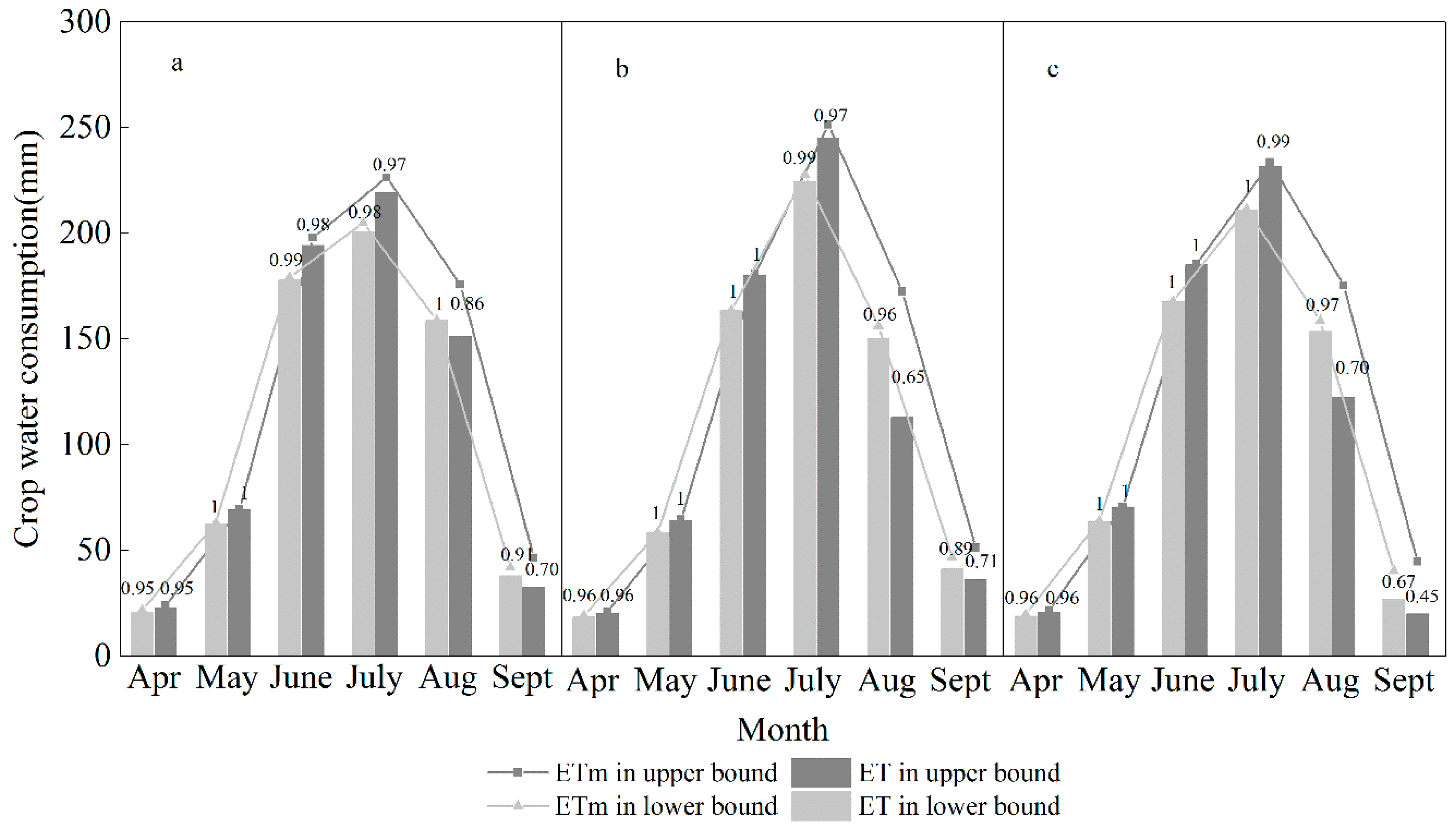
When irrigation water resources are limited, it is very necessary and meaningful to optimize the irrigation schedule over the crop growth period to obtain the maximum benefit. Taking p = 0 as example, the ratio of actual crop evapotranspiration to maximum evapotranspiration during the whole growth period for the lower and upper bounds of a wet year, normal year, dry year are shown in Figure 5. Results indicate that there is almost no water stress in May, June, and July (April is short, and the early stage of growth is of no consideration). On the other hand, in the case of insufficient irrigation water, the priority to meet maize water demand is from May to July, followed by August, and lastly September. The phenomenon is reasonable because maize yield is more sensitive to water stress in May, June, and July. In addition, yield is closely related to the water amount of irrigation. Maize depends only on irrigating more water to meet the water need of growth in arid and semi-arid zones, where precipitation is relatively small and evapotranspiration is higher. Figure 5 also indicates that maize affected by water stress in the lower bound is weaker than the upper bound. This needs a greater irrigation amount to address climate warming which leads to excessive evaporation.
4.1.4. Irrigation Water Allocation in Different Months of Different Hydrological Years
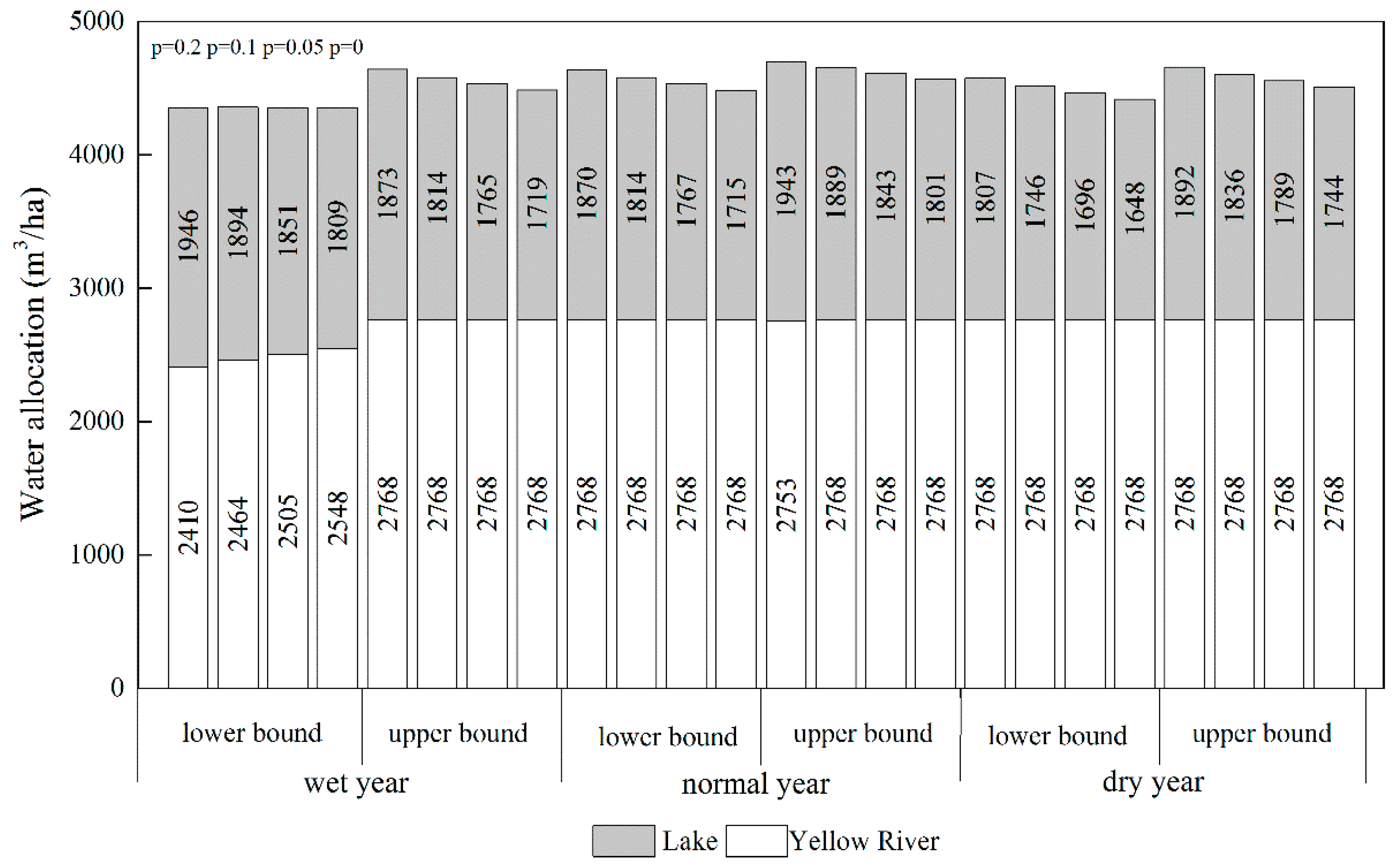
Figure 6 shows the upper bound and the lower bound of irrigation water allocation in different months for maize, which can describe the uncertainty of parameters (p = 0). The total irrigation amounts for maize under a wet year, normal year, and dry year are [4357.0, 4487.1] m3/ha, [4482.7, 4569.0] m3/ha, and [4416.1, 4512.1] m3/ha, respectively. The irrigation amount in the wet year is smaller than the dry year, and the most in the normal year. The irrigation amount is mainly affected by temperature, humidity, and other meteorological factors; therefore, it has no direct relationship with typical hydrological years. The interval results provide policy makers with more options, according to preferences and actual conditions in irrigation systems. For instance, taking the normal year as an example, the total water allocation is 4525.9 m3/ha applying to the deterministic model, however, policy makers can select any water allocation project from a range (from 4482.7 m3/ha to 4569.0 m3/ha) adopting an uncertainty model, instead of a deterministic number. In other words, the policy makers would choose the lower bound of water allocation to address climate warming because climate warming leads to excessive evaporation; therefore, water diversion from the lake becomes less. Meanwhile, lower system benefits may be obtained.
The total water allocation from May to July accounts for more than 80% of the entire growth period. The water allocation tendency is also consistent with crop water consumption (Figure 5). Although the monthly water diversion from the YR and the lake are different, the rule of irrigation water priority must be kept to meet the crop water demand in June and July, mainly using lake water in June and Yellow River water in July, and a mutual complement when the water is insufficient. Second, use the lake water for irrigation in the early months in case part of the water amount is wasted by evaporation on the premise of achieving maximum benefit. After completing the allocation of lake water in May, June, and July, the remaining Yellow River water was allocated in August. The dry matter of maize reaches the maximum value and the growth of maize depends only on rainfall in September; therefore, irrigation occurred in August instead of September. Such results are beneficial for arid and semi-arid regions, where water shortages are the major restrictive factor of ecologically sustainable development.
4.2. Comparison between the IFSSOP Model and the IFSSOP-NG Model
Generally, crop water use and irrigation scheduling decisions ignore groundwater contributions [43,44]. Hence, this research compares the optimal irrigation water allocation results of the IFSSOP model with the IFSSOP model without considering evaporation from groundwater and percolation to the groundwater (IFSSOP-NG model). The constraints of the IFSSOP-NG model and the IFSSOP model are alike.
Both the upper bound and the lower bound of the total system benefit of the IFSSOP model are higher than those of the IFSSOP-NG model for any hydrological years. In contrast, the water allocation amount to maize is less (Figure 7). The total average water allocation results of the IFSSOP model are 4422 m3/ha, 4526 m3/ha, and 4464 m3/ha for the wet year, normal year, and dry year respectively, with 4649 m3/ha, 4581 m3/ha, and 4579 m3/ha for the IFSSOP-NG model. Compared with the two models, the IFSSOP-NG model has a preference to use as much lake water as possible for the greater system benefit; however, the IFSSOP-NG model overrated the available lake water amount that would lead to inaccurate irrigation scheduling. The system benefit for maize obtained from the IFSSOP model is higher than the IFSSOP-NG model solution.
4.3. Analysis of Agriculture Water Saving Potential with IFSSOP Model
A water consumption of a 10,000 RMB output value consumes approximately 531.53 and 70 m3 in agriculture and industry, respectively [45]. The redistribution of saved water from agriculture to industry or service industry will be a huge augmenter in most developing countries [46]. On paper, agricultural water saving potential is defined as the Yellow River water saving amount adopting lake water to irrigate for the total benefit of agriculture. According to local government, the Yellow River water amount for irrigation in agriculture can be transferred to industry at a certain price (water right transfer price). The water right transfer price is 0.3 Yuan/m3 in the study region [47]. Different water saving potential scenarios are considered in order to study the relationship between agriculture water saving potential and system economic benefit more directly. In the scenarios, the percentage of water amount accounting for the total water supply amount was set up (100%, 90%, 80%, 70%, 60%, 50%, 40%, and the water deficit irrigation ratio without LW).
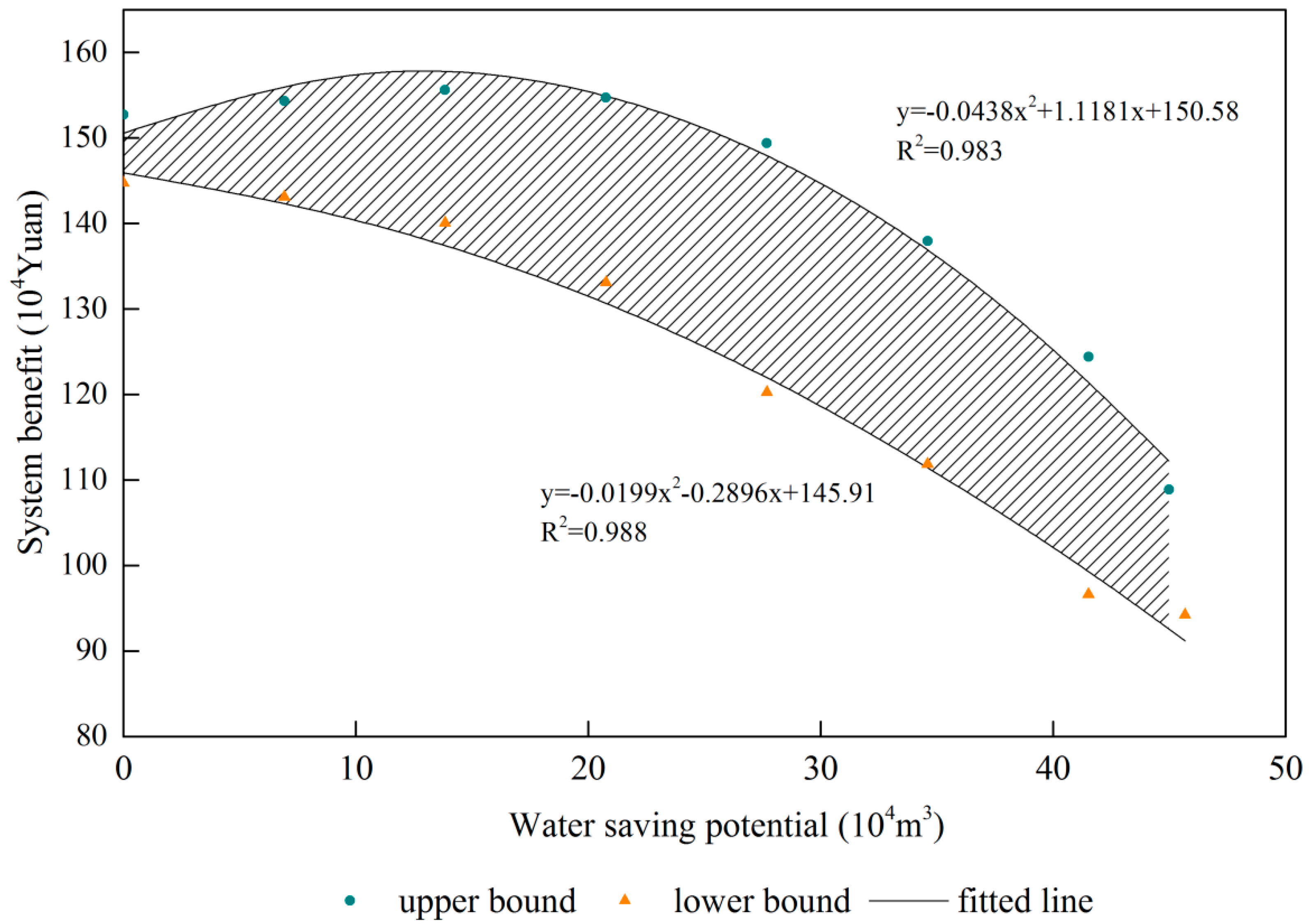
Optimized water saving potential solutions are achieved by changing the YR water supply. The two lines shown in Figure 8 compose an interval linear function of the correlation between the water saving potential and agriculture benefit, which express the uncertainties. The water saving potential-benefit curve forms a quadratic function with a maximum value, and the vertex can be used as the most profitable water saving potential scenario. This facilitates policy makers deciding upon a water saving potential in a scenario. According to the fitting curve, agriculture can save approximately 12.76 × 10⁴ m3 of YR water with maximum benefit at the upper bound, but no appropriate result at the lower bound. The results suggest that there is not enough YR irrigation water converting to industrial water under certain water shortages. The results also show that by maintaining the original crop water deficit irrigation ratio, the region can save 30–34% of the Yellow River, approximately [44.98, 45.67] × 104 m3.
5. Conclusions
An inexact fuzzy stochastic simulation-optimization programming (IFSSOP) model was developed to aid multi-water resources allocation. The developed model has two main advantages compared with the existing model. First, the model can handle uncertainty parameters. Second, it combines the field water cycle process. The developed model was applied to a case study in the Hetao Irrigation District of the upper Yellow River basin. The model was successfully used to realize the dynamic distribution of multi-water resources in an irrigation system and improve the accuracy and persuasion of the crop irrigation system optimization model. The model is useful, especially for arid regions with shallow groundwater, where water shortages have become the major constraint for economic and ecologically sustainable development.
A series of monthly crop irrigation water allocation results under different p and different hydrological years is proposed. Different scenarios lead to varied allocation results and system benefits. The results can provide different schemes for policy makers. The system benefit for maize obtained from the IFSSOP model is higher than the IFSSOP-NG model solution; the result indicates that the IFSSOP model is more precise for allocating irrigation water in a more efficient way in arid and semi-arid regions. Therefore, this is in agreement with the view of Wallender and other scholars, studying the contribution of groundwater to crop water consumption that it is important for making reasonable irrigation systems in arid and semi-arid areas with shallow groundwater [48]. For a water-saving potential analysis, it is pleasing to obtain a function between agriculture system benefit and water saving potential. The result shows YR water can be saved with maximum benefit at the upper bound. This is similar to the finding of Zhang and Qtaishat, reallocating water from irrigation to other higher-value uses such as industry or service industry can obtain its potential economic value [45,49]. It is quite meaningful to evaluate the irrigation water saving potential under the maximum benefits.
In our study, only one crop (maize) was covered in the model. Crop diversity will enhance the model complexity and have an effect on the model results. Future work will develop this model to adapt to a multi-crop irrigation system.
Acknowledgments
This research was supported by the National Key Research and Development Program of China (2017YFC0403301) and National Natural Science Fund of China (51639009, 51679236). We are grateful the editors and anonymous reviewers who contributed comments and suggestions to improve the article.
Author Contributions
Zailin Huo was responsible for the idea of the study; Xuemin Li developed the model and wrote the paper; Bing Xu provided information of the study area.
Conflicts of Interest
The authors declare no conflict of interest.
References
- Sun, S.K.; Wang, Y.B.; Wang, F.F.; Liu, J.; Luan, X.B.; Li, X.L.; Zhou, T.W.; Wu, P.T. Alleviating Pressure on Water Resources: A new approach could be attempted. Sci. Rep. 2015, 5, 14006. [Google Scholar] [CrossRef] [PubMed]
- United Nations Environment Programme (UNEP). Food Security Report; UNEP: Stockholm, Sweden, 2012. [Google Scholar]
- Akhtar, F.; Tischbein, B.; Awan, U.K. Optimizing deficit irrigation scheduling under shallow groundwater conditions in lower reaches of Amu Darya River Basin. Water Resour. Manag. 2013, 27, 3165–3178. [Google Scholar] [CrossRef]
- Flinn, J.C.; Musgrave, W.F. Development and analysis of input-output relations for irrigation water. Aust. J. Agric. Econ. 1967, 11, 127–137. [Google Scholar] [CrossRef]
- Rao, N.H.; Sarma, P.B.S. Optimal multicrop allocation of seasonal and intraseasonal irrigation water. Water Resour. Res. 1990, 26, 551–559. [Google Scholar] [CrossRef]
- Vedula, S.; Kumar, D.N. An integrated model for optimal reservoir operation for irrigation of multiple crops. Water Resour. Res. 1996, 32, 1101–1108. [Google Scholar] [CrossRef]
- Wong, H.S.; Sun, N.Z.; Yeh, W.W.-G. A Two-Step Nonlinear Programming Approach to the Optimization of Conjunctive Use of Surface Water and Ground Water; University of California Water Resources Center: Davis, CA, USA, 1997. [Google Scholar]
- Shangguan, Z.P.; Shao, M.G.; Horton, R.; Lei, T.W.; Qin, L.; Ma, J.Q. A model for regional optimal allocation of irrigation water resources under deficit irrigation and its applications. Agric. Water Manag. 2002, 52, 139–154. [Google Scholar] [CrossRef]
- Bijan, G.; Ali-Reza, S. Linear and Non-Linear optimization models for allocation of a limited water supply. Irrig. Drain. 2004, 53, 39–54. [Google Scholar] [CrossRef]
- Regulwar, D.G.; Gurav, J.B. Irrigation planning under uncertainty—A multi objective fuzzy linear programming approach. Water Resour. Manag. 2011, 25, 1387–1416. [Google Scholar] [CrossRef]
- Zhang, X.D.; Huang, G.H.; Nie, X.H.; Lin, Q.G. Model-based decision support system for water quality management under hybrid uncertainty. Expert Syst. Appl. 2011, 38, 2809–2816. [Google Scholar] [CrossRef]
- Sethi, L.N.; Panda, S.N.; Nayak, M.K. Optimal crop planning and water resources allocation in a coastal groundwater basin, Orissa, India. Agric. Water Manag. 2006, 83, 209–220. [Google Scholar] [CrossRef]
- Lu, H.W.; Huang, G.H.; He, L. An inexact rough-interval fuzzy linear programming method for generating conjunctive water-allocation strategies to agricultural irrigation systems. Appl. Math. Model. 2011, 35, 4330–4340. [Google Scholar] [CrossRef]
- Mahmood, S.S.; Mostafa, M. Application of Robust Optimization Approach for Agricultural Water Resource Management under Uncertainty. J. Irrig. Drain. 2013, 139, 571–581. [Google Scholar] [CrossRef]
- Li, M.; Guo, P. A multi-objective optimal allocation model for irrigation water resources under multiple uncertainties. Appl. Math. Model. 2014, 38, 4897–4911. [Google Scholar] [CrossRef]
- Li, W.; Wang, B.; Xie, L.Y.; Huang, G.H.; Liu, L. An inexact mixed risk-aversion two-stage stochastic programming model for water resources management under uncertainty. Environ. Sci. Pollut. Res. 2015, 22, 2964–2975. [Google Scholar] [CrossRef] [PubMed]
- Yang, G.Q.; Guo, P.; Li, M.; Fang, S.Q.; Zhang, L.D. An improved solving approach for interval-parameter programming and application to an optimal allocation of irrigation water problem. Water Resour. Manag. 2016, 30, 701–729. [Google Scholar] [CrossRef]
- Maqsood, I.; Huang, G.H.; Yeomans, J.S. An interval-parameter fuzzy two-stage stochastic program for water resources management under uncertainty. Eur. J. Oper. Res. 2005, 167, 208–225. [Google Scholar] [CrossRef]
- Han, Y.; Huang, Y.F.; Wang, G.Q. Interval-parameter linear optimization model with stochastic vertices for land and water resources allocation under dual uncertainty. Environ. Eng. Sci. 2011, 28, 197–205. [Google Scholar] [CrossRef]
- Nevill, C.J. Managing cumulative impacts: Groundwater reform in the Murray-Darling Basin, Australia. Water Resour. Manag. 2009, 23, 2605–2631. [Google Scholar] [CrossRef]
- Harmancioglu, N.B.; Barbaros, F.; Cetinkaya, C.P. Sustainability issues in water management. Water Resour. Manag. 2013, 27, 1867–1891. [Google Scholar] [CrossRef]
- Cosgrove, D.M.; Johnson, G.S. Aquifer management zones based on simulated surface-water response functions. J. Water Resour. Plan. Manag. 2005, 131, 89–100. [Google Scholar] [CrossRef]
- Safavi, H.R.; Alijanian, M.A. Optimal crop planning and conjunctive use of surface water and groundwater resources using fuzzy dynamic programming. J. Irrig. Drain. Eng. 2011, 137, 383–397. [Google Scholar] [CrossRef]
- Lu, H.W.; Huang, G.H.; Zhang, Y.M.; He, L. Strategic agricultural land-use planning in response to water-supplier variation in a China’s rural region. Agric. Syst. 2012, 108, 19–28. [Google Scholar] [CrossRef]
- Shi, B.; Lu, H.W.; Ren, L.X.; He, L. A fuzzy inexact two-phase programming approach to solving optimal allocation problems in water resources management. Appl. Math. Model. 2014, 38, 5502–5514. [Google Scholar] [CrossRef]
- Guo, P.; Chen, X.H.; Tong, L.; Li, J.B.; Li, M. An optimization model for a crop deficit irrigation system under uncertainty. Eng. Opt. 2014, 46, 1–14. [Google Scholar] [CrossRef]
- Ren, D.Y.; Xu, X.; Hao, Y.Y.; Huang, G.H. Modeling and assessing field irrigation water use in a canal system of Hetao, upper Yellow River basin: Application to maize, sunflower and watermelon. J. Hydrol. 2016, 532, 122–139. [Google Scholar] [CrossRef]
- Gao, X.Y.; Huo, Z.L.; Bai, Y.N.; Feng, S.Y.; Huang, G.H.; Shi, H.B.; Qu, Z.Y. Soil salt and groundwater change in flood irrigation field and uncultivated land: A case study based on 4-year field observations. Environ. Earth Sci. 2015, 73, 2127–2139. [Google Scholar] [CrossRef]
- Xu, X.; Huang, G.H.; Qu, Z.Y.; Pereira, L.S. Assessing the groundwater dynamics and impacts of water saving in the Hetao Irrigation District, Yellow River basin. Agric. Water Manag. 2010, 98, 301–313. [Google Scholar] [CrossRef]
- Zhang, Z.J.; Yang, S.Q.; Shi, H.B.; Ma, J.H.; Li, R.P.; Han, W.G.; Zhang, W.J. Irrigation infiltration and recharge coefficient in Hetao irrigation district in Inner Mongolia. Trans. CSAE 2011, 27, 6–66. [Google Scholar]
- Hu, S.J.; Zhao, R.F.; Tian, C.Y.; Song, Y.D. Empirical models of calculating phreatic evaporation from bare soil in Tarim river basin, Xinjiang. Environ. Earth Sci. 2009, 59, 663–668. [Google Scholar] [CrossRef]
- Chen, D.L.; Gao, G.; Xu, C.Y.; Guo, J.; Ren, G.Y. Comparison of the Thornthwaite method and pan data with the standard Penman-Monteith estimates of reference evapotranspiration in China. Clim. Res. 2005, 28, 123–132. [Google Scholar] [CrossRef]
- Hao, F.H.; Ou, Y.W.; Yue, W. Analysis of water cycle characteristics and soil water movement in the agricultural irrigation area in Inner Mongolia. Acta Sci. Circumst. 2008, 5, 825–831. [Google Scholar]
- Ren, Z.H.; Li, M.Q.; Zhang, W.M. Conversion Coefficient of SMAII Evaporation PAN into E-601B PAN in China. J. Appl. Meteorol. Sci. 2002, 4, 508–514. [Google Scholar]
- Allen, R.G.; Pereira, L.S.; Raes, D.; Smith, M. Crop Evapotranspiration: Gudelines for Computing Crop Water Requirements, Irrigation and Drainage 56; United Nations (FAO): Rome, Italia, 1998. [Google Scholar]
- Tsakiris, G.P. A method for applying crop sensitivity factors in irrigation scheduling. Agric. Water Manag. 1982, 5, 335–343. [Google Scholar] [CrossRef]
- Wang, Y.R.; Lei, Z.D.; Yang, S.X. Cumulative function of sensitive index for winter wheat. J. Hydraul. Eng. 1997, 5, 29–36. [Google Scholar]
- Zhang, X.Y.; Chen, S.Y.; Sun, H.Y.; Shao, L.W.; Wang, Y.Z. Changes in evapotranspiration over irrigated winter wheat and maize in North China Plain over three decades. Agric. Water Manag. 2011, 98, 1097–1104. [Google Scholar] [CrossRef]
- Li, M.; Guo, P.; Singh, V.P. An efficient irrigation water allocation model under uncertainty. Agric. Syst. 2016, 144, 46–57. [Google Scholar] [CrossRef]
- Zimmermann, H.J. Fuzzy Set Theory and Its Applications, 3rd ed.; Kluwer Academic Publishers: Boston, MA, USA, 1996; ISBN 9780792396246. [Google Scholar]
- Li, Y.P.; Huang, G.H.; Wang, G.Q.; Huang, Y.F. FSWM: A hybrid fuzzy-stochastic water management model for agricultural sustainability under uncertainty. Agric. Water Manag. 2009, 96, 1807–1818. [Google Scholar] [CrossRef]
- Guo, P.; Huang, H.G.; He, L.; Li, H.L. Interval-parameter Fuzzy-stochastic Semi-infinite Mixed-integer Linear Programming for Waste Management under Uncertainty. Environ. Model. Assess. 2009, 14, 521–537. [Google Scholar] [CrossRef]
- Hanson, B.R.; Kite, S.W. Irrigation scheduling under saline high water tables. Trans. ASABE 1984, 27, 1430–1434. [Google Scholar] [CrossRef]
- Ayars, J.E.; Hutmacher, R.B. Crop coefficients for irrigating cotton in the presence of groundwater. Irrig. Sci. 1994, 15, 45–52. [Google Scholar] [CrossRef]
- Zhang, D.M.; Guo, P. Integrated agriculture water management optimization model for water saving potential analysis. Agric. Water Manag. 2016, 170, 5–19. [Google Scholar] [CrossRef]
- Gohari, A.; Eslamian, S.; Mirchi, A.; Abedi-Koupaei, J.; Bavani, A.M.; Madani, K. Water transfer as a solution to water shortage: A fix that can Backfire. J. Hydrol. 2013, 491, 23–39. [Google Scholar] [CrossRef]
- Wang, L.M.; Li, Y. The overall planning of the Yellow River water rights conversion in Inner Mongolia. Inn. Mong. Water Conserv. 2005, 1, 55–56. [Google Scholar]
- Wallender, W.W.; Grimes, D.W.; Henderson, D.W.; Stromberg, L.K. Estimating the Contribution of a Perched Water Table to the Seasonal Evapotranspiration of Cotton. Agron. J. 1979, 71, 1056–1060. [Google Scholar] [CrossRef]
- Qtaishat, T. Impact of Water Reallocation on the Economy in the Fertile Crescent. Water Res. Manag. 2013, 27, 3765–3774. [Google Scholar] [CrossRef]
Figure 1.
The location of the study region.
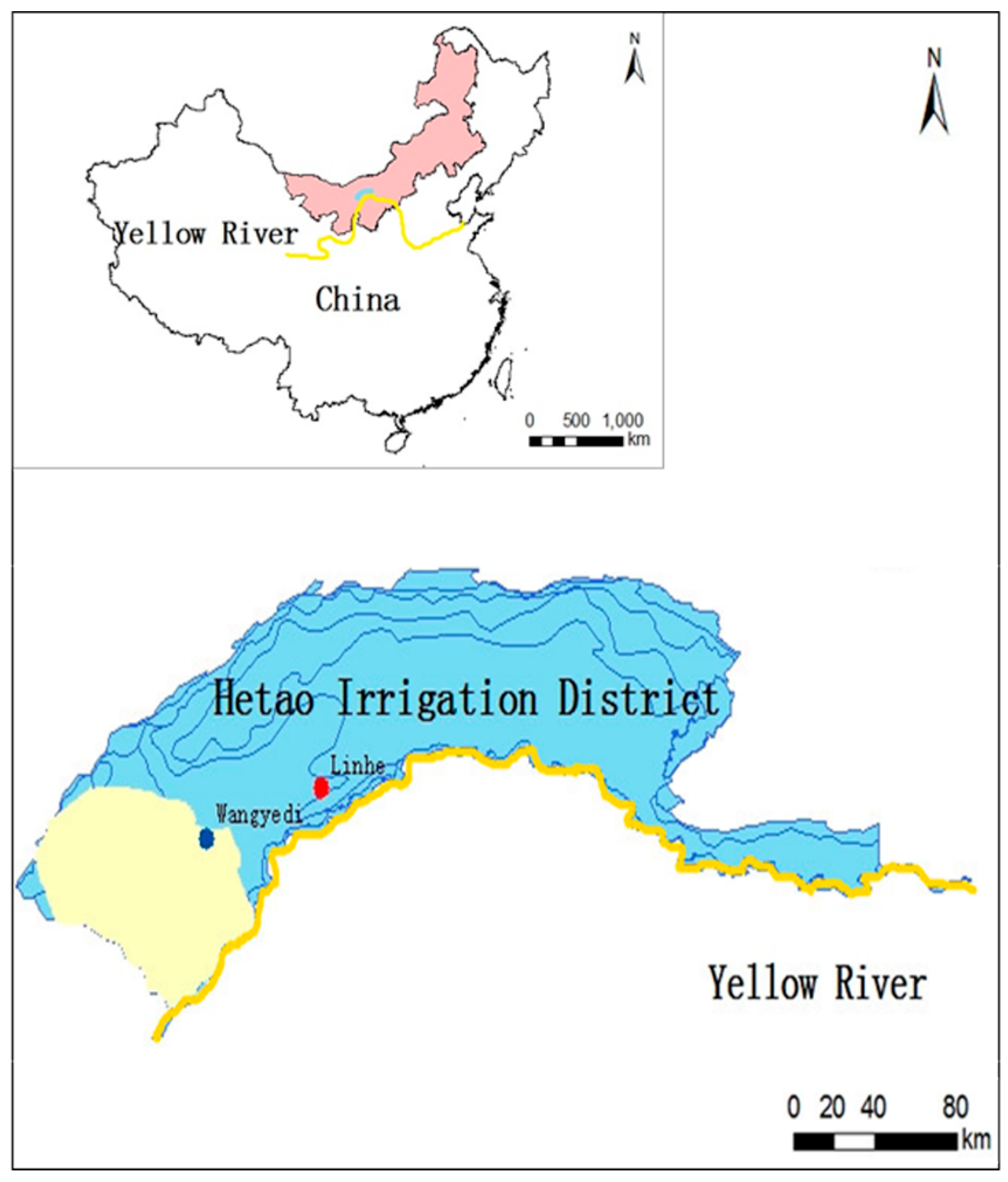
Figure 2.
Schematic of the simulation-optimization model for irrigation system: P is precipitation; ET, E0 and ETg are actual evapotranspiration, lake evaporation and groundwater evaporation; YI and LI are irrigation from the Yellow River and lake, respectively; G is ice flood; Dinf is irrigation infiltration; R is the exchange capacity of groundwater and lake.
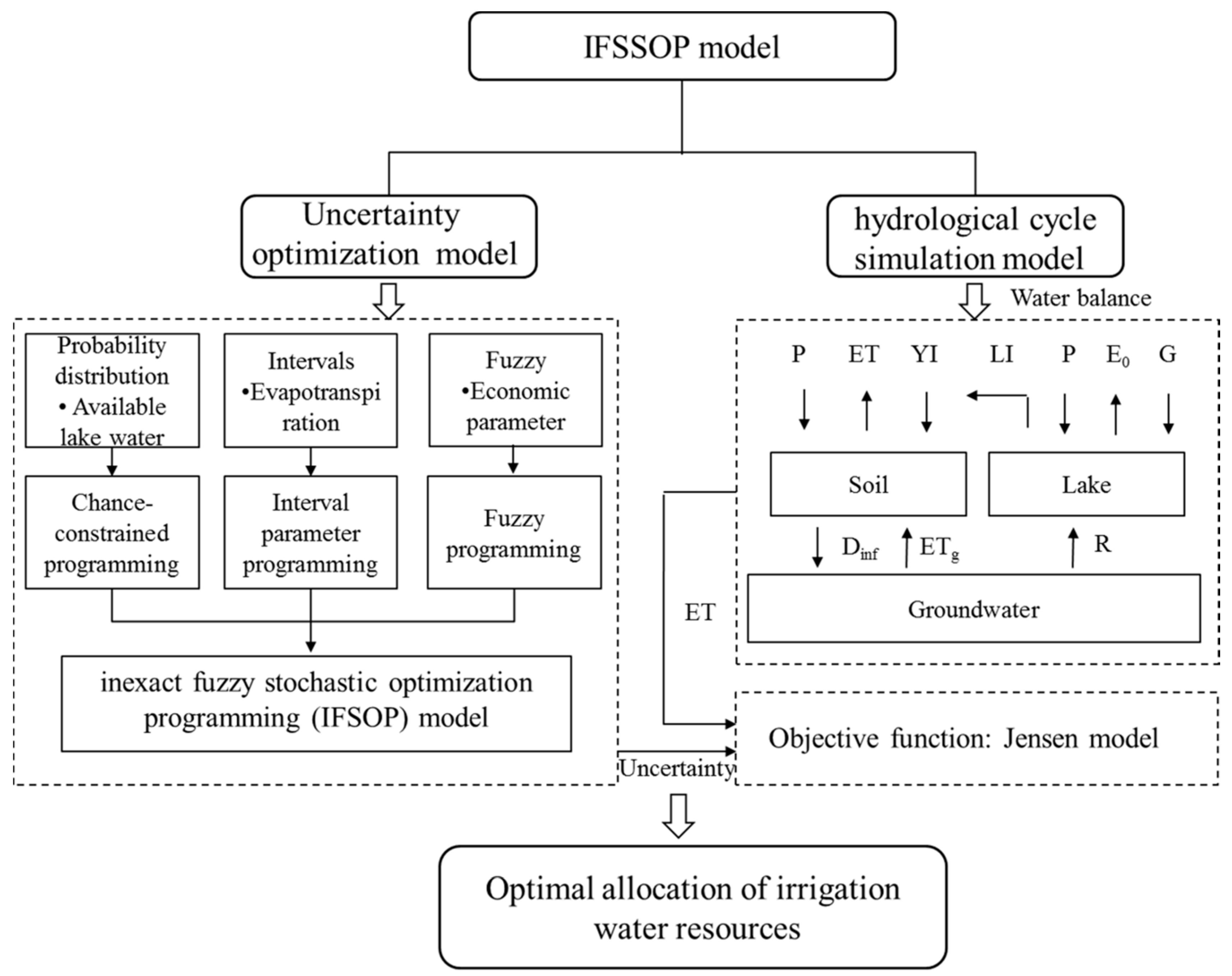
Figure 3.
The optimal irrigation water allocation of two water sources under various p in different hydrological years.
Figure 3.
The optimal irrigation water allocation of two water sources under various p in different hydrological years.

Figure 4.
The total system economic benefit under different p in different hydrological years.

Figure 5.
Monthly crop water consumption and the proportion of the actual crop consumption to the maximum crop consumption: wet year (a); normal year (b) and dry year (c).
Figure 5.
Monthly crop water consumption and the proportion of the actual crop consumption to the maximum crop consumption: wet year (a); normal year (b) and dry year (c).

Figure 6.
Monthly irrigation water allocation schemes in different hydrological years: (a) is wet year; (b) is normal year; (c) is dry year. Lower bound and upper bound of water allocation from left to right.
Figure 6.
Monthly irrigation water allocation schemes in different hydrological years: (a) is wet year; (b) is normal year; (c) is dry year. Lower bound and upper bound of water allocation from left to right.
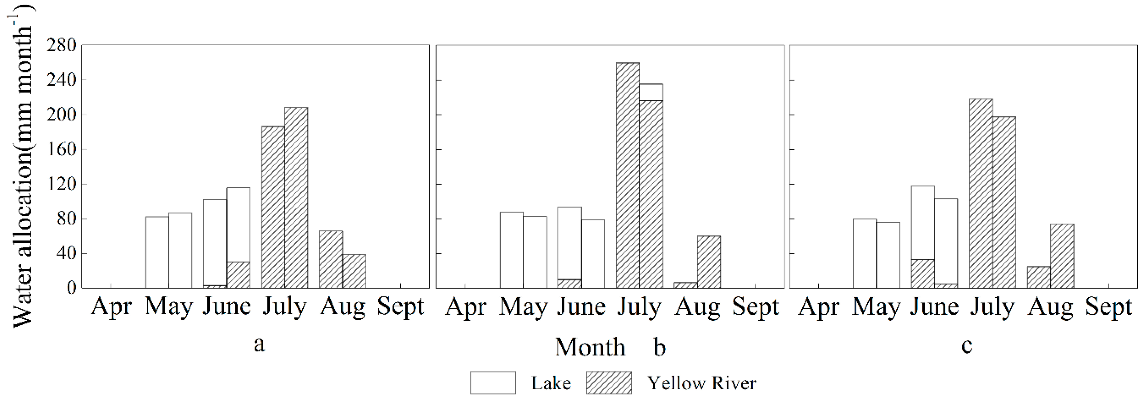
Figure 7.
Comparison between IFSSOP model and IFSSOP-NG model.
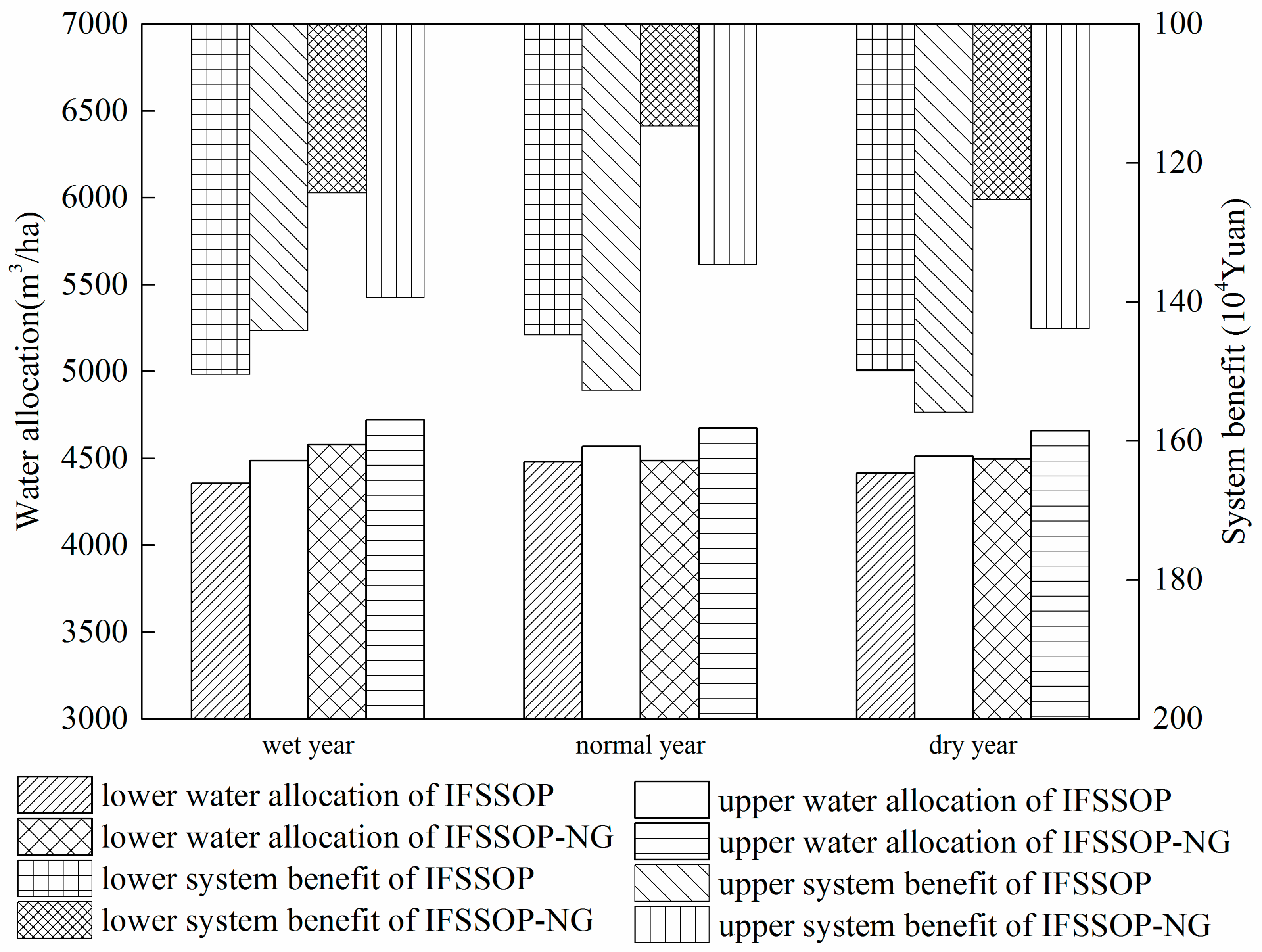
Figure 8.
Optimization solutions under different scenarios (100%, 90%, 80%, 70%, 60%, 50%, 40% of total water amount and original water deficit irrigation ratio).
Figure 8.
Optimization solutions under different scenarios (100%, 90%, 80%, 70%, 60%, 50%, 40% of total water amount and original water deficit irrigation ratio).


Table 1.
Fitting ETm and λ value of maize in different months.
| Hydrological Year | Month | 4 | 5 | 6 | 7 | 8 | 9 |
|---|---|---|---|---|---|---|---|
| λ | 0.01 | 0.05 | 0.14 | 1.31 | 0.03 | 0.01 | |
| Wet year | ETm (mm) | [21.54, 23.80] | [62.84, 69.45] | [179.03, 197.87] | [204.78, 226.34] | [158.79, 175.51] | [41.81, 46.21] |
| Normal year | ETm (mm) | [19.79, 21.08] | [60.53, 64.46] | [169.51, 80.58] | [236.02, 251.35] | [161.86, 172.39] | [48.07, 51.20] |
| Dry year | ETm (mm) | [19.60, 21.67] | [63.92, 70.65] | [167.69, 185.34] | [211.30, 233.55] | [158.49, 175.18] | [40.21, 44.44] |
Note: λ means the sensitive index, ETm means the maximum crop evapotranspiration in a month (interval number).
© 2017 by the authors. Licensee MDPI, Basel, Switzerland. This article is an open access article distributed under the terms and conditions of the Creative Commons Attribution (CC BY) license (http://creativecommons.org/licenses/by/4.0/).
Share and Cite
MDPI and ACS Style
Li, X.; Huo, Z.; Xu, B. Optimal Allocation Method of Irrigation Water from River and Lake by Considering the Field Water Cycle Process. Water 2017, 9, 911. https://doi.org/10.3390/w9120911
AMA Style
Li X, Huo Z, Xu B. Optimal Allocation Method of Irrigation Water from River and Lake by Considering the Field Water Cycle Process. Water. 2017; 9(12):911. https://doi.org/10.3390/w9120911
Chicago/Turabian StyleLi, Xuemin, Zailin Huo, and Bing Xu. 2017. "Optimal Allocation Method of Irrigation Water from River and Lake by Considering the Field Water Cycle Process" Water 9, no. 12: 911. https://doi.org/10.3390/w9120911
Note that from the first issue of 2016, this journal uses article numbers instead of page numbers. See further details here.