Effects of Using High-Density Rain Gauge Networks and Weather Radar Data on Urban Hydrological Analyses

WISE Institute, Hankuk University of Foreign Studies, Yongin-si, Gyeonggi-do 17035, Korea
*
Author to whom correspondence should be addressed.
Water 2017, 9(12), 931; https://doi.org/10.3390/w9120931
Submission received: 7 October 2017
/
Revised: 27 November 2017
/
Accepted: 28 November 2017
/
Published: 29 November 2017
Abstract
:Flood prediction is difficult in urban areas because only sparse gauge data and radar data of low accuracy are usually used to analyze flooding and inundation. Sub-basins of urban areas are extremely small, so rainfall data of high spatial resolution are required for analyzing complex drainage systems with high spatial variability. This study aimed to produce three types of quantitative precipitation estimation (QPE) products using rainfall data that was derived from 190 gauges, including the new high-density rain-gauge network operated by the SK Planet company, and the automated weather stations of the Korea Meteorological Administration, along with weather radar data. This study also simulated urban runoff for the Gangnam District of Seoul, South Korea, using the obtained QPE products to evaluate hydraulic and hydrologic impacts according to three rainfall fields. The accuracy of this approach was assessed in terms of the amount and spatial distribution of rainfall in an urban area. The QPE products provided highly accurate results and simulations of peak runoff and overflow phenomena. They also accurately described the spatial variability of the rainfall fields. Overall, the integration of high-density gauge data with radar data proved beneficial for quantitative rainfall estimation.
1. Introduction
Recent climate change and abnormal weather phenomena have resulted in increased occurrences of localized torrential rainfall in South Korea, including urban areas. The urban hydrological environment has changed in relation to precipitation, in terms of reduced concentration time, decreased storage rate, and increased peak discharge. These changes have altered and increased the severity of damage to urban areas. The notable recent Seoul floods in 2010 and 2011 are examples of such disasters [1]. Accordingly, extensive research has been conducted on urban flood forecasting using only point rain gauges; however, this approach is inadequate for developing efficient disaster prevention measures, as such gauges, can not detect the spatial variations in rainfall [2].
The mean areal precipitation (MAP) is usually used as input to hydrologic and hydraulic models. When MAP is measured with a low-density gauge network, noticeable errors are found in the simulated peak discharge [3,4]. Previous studies have confirmed that the spatial resolution of rainfall data substantially affects rainfall runoff simulations [5]. In particular, previous rainfall and hydrologic studies in urban basins, using high-density rain-gauge networks, have mentioned the necessity of accurately measuring intense heavy rainfall that is occurring in a specific area over a short period of time, and using spatially distributed rainfall for urban flood analysis [6,7]. However, it is not always realistic to install numerous rain gauges to measure spatially representative rainfall estimates over a metropolitan area for geographic and economic reasons [8]. Therefore, various researchers have attempted to use radar rainfall data. Nevertheless, the results of studies using radar rainfall data to prevent urban flood disasters in Korea were found to be inefficient because of the low accuracy and low spatial resolution of these radar rainfall data.
For the design and analysis of urban hydrological systems, rainfall data should have minimum temporal and spatial resolutions of 5 min and 1 km2, respectively. Furthermore, the uncertainty of rainfall intensity should be less than 10%, and within a range of 10–50 mm/h [9]. In particular, recent research has suggested a minimum resolution of 1 min/100 m for smaller catchments with an area of 0.01 km2 or less [10]. Urban areas are usually divided into small catchments for urban hydrological applications; therefore, the use of high-resolution radar data is recommended [11].
Thus far, research on urban flood estimation and forecast has mostly employed radar data as inputs to a hydrological model. James et al. [12] studied flood forecasting using radar and gauge data on the Yockanookany watershed of the Mississippi River in the United States (U.S.) The results showed that the accuracy of the hydrographs was improved after the radar data were calibrated, using gauge data based on a Kriging coefficient method. Pessoa et al. [13] used a Distributed Basin Simulation model (DBS) to test the sensitivity of rainfall estimations to radar data input. They reported that flood estimation was improved because the radar provided more accurate average rainfall accumulations and improved the determined spatial distribution of rainfall. Improved flood forecasting results were obtained by Mimikou and Baltas [14] by using both radar and gauge rainfall data as inputs to the HEC-1 (Hydrologic Engineering Center) rainfall-runoff model. Sun et al. [15] compared flood forecast results with different rainfall estimates, including those from rain-gauge data alone, Kriging of rain-gauge data, radar data alone, and co-Kriging of both radar and rain-gauge data. They concluded that rainfall that was estimated by the co-Kriging method considerably improved flood estimation. Therefore, rainfall data have also been obtained from weather radars for hydrological applications. Kim et al. [16] used various approaches combining radar and rain gauges, including Kriging of rain-gauge data alone, using only radar data, using the mean-field bias of both radar and rain gauges, and the conditional merging of both radar and rain gauges. Subsequently, they evaluated the performance of flood estimates with the product of these approaches using a physics-based distributed hydrologic model. Their results showed that the conditional Kriging method provided the most accurate results for flood estimation.
As shown in the literature review, ground-observed rainfall is necessary for the improved accuracy of radar-estimated rainfall in order to reflect the true quantitative value. For this purpose, various techniques have been suggested to improve the accuracy of radar rainfall estimates by using rain gauges [17,18]. One approach is to merge radar estimates with gauge measurements operationally in order to obtain quantitatively accurate and spatially continuous radar-derived rainfall fields [19,20]. Past studies have shown the necessity of denser rain-gauge networks for improving the accuracy of radar rainfall field data. In the past, rain gauges were quite scarce in urban areas; however, high-density networks have been recently established over wide areas, such as in metropolitan cities, states, and countries, for research and commercial purposes. In the U.S., Japan, and other countries, telecommunication companies have built local observation networks to provide meteorological information. Using the base stations of these companies saves additional costs related to the transmission of data, because the networks are already established and the stations provide optimal locations for gauge system installation without any surrounding canopy (vegetation and trees). For example, WeatherBug operates the large surface weather network in the world with over 8000 surface weather stations across the U.S.; the observed data are used for severe-weather prediction [21]. Minnesota’s high-density rain gauge network combines many observer organizations with different aims and different instruments for estimating extreme rainfall frequencies, using 45 years of observed daily rainfall [22]. NTT Docomo, which is a major telecommunications company in Japan, established an environmental sensor network for its 4000 mobile network base stations around the country in 2011 and 2012. The stations are approximately 10 km from each other and the installed equipment observes temperature, humidity, direction and speed of wind, and precipitation for weather forecasting and disaster mitigation [23]. Currently, SK Planet (SKP), a subsidiary of SK Telecommunication Company in Korea, has established 1089 weather observatory facilities in the Seoul region. Compared to other high-density observation networks, SKP created the world’s densest weather observatory network with similar or newer equipment.
The aims of this study were to produce quantitative precipitation estimation (QPE) products by using data from the densest rain gauge network and weather radar data, and to analyze the effect of high rain-gauge density and radar data in terms of the amount and spatial distribution of rainfall. The availability of QPE products for urban runoff simulation was also analyzed. The objectives were (I) to produce and assess high-resolution QPE products for Seoul, using high-density observed rainfall and radar rainfall data and (II) to assess the applicability of the simulated runoff with QPE products using an urban runoff model. The study area, data sources, and methodologies are explained in Section 2, and the storm water management model is presented in Section 3. The results of the QPE products according to high gauge density and radar data in terms of urban runoff analysis are presented for a rainfall event in Section 4 and the conclusions are presented in Section 5.
2. Study Area and Data
2.1. Study Area
The study area is located in the Gangnam District of Seoul, the capital of South Korea. It covers an area of 605 km2 (126°46′15″ to 127°11′15″ E longitude, 37°25′50″ to 37°41′45″ N latitude; Figure 1a). Seoul is one of the most highly urbanized cities in Korea; impervious areas reached 48.64% of the total urban area in 2014. In addition, several residential areas and industrial facilities are located near flood plains, such that the damage that is caused by urban flooding is exacerbated. For instance, Seoul experienced heavy rainfall events in 2010 and 2011. One of these (26–29 July 2011) resulted in 67 casualties and 37.7 billion KRW (Korea Republic Won) worth of property damage, which amounted to 50% of the total damage that was caused by natural disasters in Korea in 2011. Moreover, the greatest volume of rain among all of the rainfall events recorded since the beginning of 1908 was deposited in Korea on 21 September 2010. These torrential rains flooded 4727 residential areas, 1164 shopping areas, and 126 factories.
The drainage system of Seoul is managed by dividing it into 16 drainage zones. These are separated by the tributaries and the main outfalls of the Han River that flow directly into the river. These 16 drainage zones are further divided into 239 drainage districts within the region.
Gangnam District lies at the intersection of Gangnam-dong and Teheran-ro; it is representative of Seoul’s downtown area where residential and commercial areas are concentrated. Geomorphically, it is a relatively low-lying location with a complicated sewer network as compared to the surrounding areas. Thus, this area is vulnerable to flooding during heavy rainfall and the events in 2010 and 2011 caused flood damage to it. Gangnam has five drainage districts (Nonhyeon, Yeoksam, Seocho 1, Seocho 2, and Seocho 3), which collectively cover an area of 7.4 km2. The drainage system comprises 4170 manholes, pipelines with a total length of 200,698 km, and two drainage pump systems at the Sapyeong and Seocho stations (indicated by black boxes in Figure 1b).
2.2. High-Density Rain-Gauge Network
In Korea, weather observations are traditionally carried out through the observation network of the Korea Meteorological Administration (KMA). This network has 95 automated surface observing systems (ASOS) and 493 automatic weather stations (AWSs) nationwide. Of these stations, 34 are used for meteorological observations in Seoul.
In recent years, SKP has been operating an integrated meteorological sensor network, using the base station infrastructure of the SK Telecom company. This network provides meteorological information, thereby offering weather services that can be used in disaster prevention. By May 2013, SKP had installed 264 operational meteorological sensors over the city of Seoul (Figure 1a), and another 131 around Incheon. In 2014, it also established 694 sensors in Gyeonggi Province. A total of 1089 meteorological sensors have been installed at intervals of 1–3 km, forming the world’s densest weather observatory network. The meteorological information that was collected by SKP can be used to enhance the accuracy of weather observations by the existing disaster prevention system. The SKP sensors are set to the KMA standard to collect meteorological data, such as from the AWS of the KMA, every minute in real time [24]. In addition, SKP regularly maintains the observed data by using automatic and semi-automatic observation information quality-management systems (www.weatherplanet.co.kr).
The data used in this study were collected through the AWSs of SKP and KMA. The data contained errors that had occurred at the AWSs, such as system malfunctions, calibration deviations, and bias errors, in addition to errors that were associated with electronic and communication malfunctions [25,26,27]. Using data with such errors decreases the accuracy of (or increases the uncertainty of) the hydrological runoff products. Therefore, data quality tests were conducted, and gauge stations with high missing rates were eliminated following a quality control technique in order to use the observed data from the AWSs of SKP and the KMA, effectively. The criteria of quality control were determined for missing values or outliers, as shown in Table 1. Here, R10min is the 10-min accumulated rainfall, Pi is the observed rainfall at station “i”, and σ is the spatial standard deviation of rain gauges within 7 km. The Madsen-Allerup method [28,29] is a non-parameterized spatial checking method that is based on analyses of median values and upper and lower quartiles of data from stations in the surrounding area. If Tit exceeds 2.0, then it is judged to be “suspicious”.
The accuracy of SKP data from 262 stations was evaluated for three months from July to September 2013, targeting the KMA data using the abovementioned criteria to ensure data stability. The time interval of observations was 1 min. The average missing ratio was 18.71% for the three months, and the missing ratio of the 262 stations ranged from 2.00% to 77.11%. Missing values were caused by system errors during wire transmission and equipment defects. In order to ensure data stability, 156 SKP stations were selected, which had less than 20% missing ratio and less than three times the average standard deviation of cumulative rainfall for three months. The cumulative rainfall average of these stations was 878.2 mm and the standard deviation (σ) was 136.6 mm for three months.
The average missing ratio, which was recorded as “null”, was 7.09% for SKP and 0.46% for KMA for three months. The density of available rain gauges was approximately 3 km2 per gauge and the average distance between rain gauges was 977 m in the Seoul area. SKP rain gauge stations nearest to the KMA stations were selected and the observed rainfall estimates were compared one-to-one. The average relative error was within 0.25% for all of the evaluated stations. The error was determined according to the difference between observation equipment and location; therefore, the accuracy of the SKP data matched that of the KMA data [30]. The 156 SKP rain gauge stations were selected among the 262 stations through the quality control and the 34 gauge stations operated by the KMA were used additionally (indicated by black stars in Figure 1a). In total, 190 rain gauge stations were used in this study.
2.3. Weather Radar Data
For the purpose of rainfall estimation in terms of spatial variability in urban areas, radar-derived rainfall was estimated using data from the Gwangdeok Weather Radar Station (GDK). The radar site is located on Gwangdeok Mountain in Gangwon Province, approximately 100 km northeast of Seoul, and it is used to investigate the three-dimensional structure of clouds. The GDK radar is an S-band type, with a beam width of 1° and a gate size of 250 m. The GDK radar data are in the Universal Format (UF), and most of the noise, such as ground, sea, sun strobe, and AP clutter, was removed using the Worldwide Integrated Sensors for Hydrometeorology group (WISH) algorithms from the Next Generation Weather Radar (NEXRAD), U.S. As there are many mountains near the radar site and study area, volume data for the radar reflectivity data were extracted to obtain constant altitude plan position indicator (CAPPI) data at a height of 1.5 km in order to eliminate ground clutter using a bilinear interpolation program, which was based on the algorithm, as suggested by Mohr and Vaughan [31]. The spherical coordinates of the volume data were transformed to Cartesian coordinates. The spatial and temporal resolutions of the extracted CAPPI data are 250 × 250 m2 and 10 min, respectively.
2.4. Drainage Network and Topographic Data
To obtain input data for urban runoff analysis, the data from pipes and manholes were collected from the Seoul drainage network map and then simplified. The pipe input data were simplified into an urban hydrological model using diameters of 600 mm and lengths of 100 m. In total, input data from 773 manholes, 1059 pipes, and 772 sub-basins were used. The Gangnam area is mostly occupied by buildings and paved streets that extend up to the foot of Umyeon Mountain. The areas of the sub-basins range between 0.0002 km2 and 0.435 km2, with an average area of 0.01 km2. There are no manholes at the sub-basins of the southwestern part of the area, including Umyeon Mountain. The slope was calculated using a digital elevation model (DEM) at a resolution of 5 m, with slopes ranging from 0.001% to 10.092%. The average slope of the northeast region is gentle and the Gangnam area is a relatively low-lying area. Furthermore, the Seoul Biotope Map was used to determine the distribution of runoff curve numbers (CN) and impermeability rates, which were 47–95 and 10.6–100%, respectively.
3. Methodology
3.1. Quantitative Precipitation Estimation
In this study, ordinary Kriging, conditional merging, and Z–R relationships were used to produce three types of QPE products. The ordinary Kriging method was used to distribute the point rainfall from the KMA and SKP AWSs. In addition, the Kriging method was used in the conditional merging method. The Kriging method involves the use of partial information to estimate the value of an unknown point through interpolation, based on the least-squares regression analysis method. To estimate the value of a point with this method, the weight of the given point needs to be determined first. Among the methods that are used to calculate a weight, ordinary Kriging uses an unbiased estimation equation and the least error variance [32,33]. The Geostatistical Software Library (Gslib) was used in this study for the computational implementation of the Kriging method, and a Gaussian model was assumed for the variogram [34].
To use only radar data, the raw radar data (dBZ) were converted into rainfall intensity data using the Z–R power-law relation (Z = aRb), with a = 200 and b = 1.6. This equation is not applicable to heavy rainfall; however, the objective of this study was to identify the usefulness of a high-density rain-gauge network for QPE. Accordingly, the Marshall-Palmer equation was selected to exclude factors that could affect accuracy. To merge the radar and rain-gauge data, the conditional merging method was used. This method is based on the assumption that rain gauges measure the amount of rainfall accurately, but only at discrete points, whereas radar data could be faulty, but provide a reliable spatial distribution of rainfall occurrences. The efficiency of this combination in reducing the bias and variance of the error estimates was evaluated through simulation experiments. The technique uses radar observations of rainfall fields to estimate errors that are associated with Kriging, and to interpolate between rain-gauge observations and the Kriged gauge fields. In this manner, the spatial information in the final merged field is improved, while the mean field characteristics that are recorded by the gauges are maintained [18,35].
The evaluation was carried out using the k-fold cross validation technique to examine improvements in the accuracy of each estimated rainfall field against the rain-gauge observations. This approach analyzes data that are first partitioned into k equally sized segments or folds. Subsequently, k iterations of training and validation are performed at each iteration, and a different fold of the data is held for validation, while the remaining k − 1 folds are used for training. A comparison of the cross validation of three types of rainfall fields (QPE1–QPE3) was made for all of the events using the following four evaluation factors: root mean squared error (RMSE), correlation with the rain-gauge data (C-CORR), mean error (ME), and the mean absolute error (MAE). In this study, where k of the k-fold cross validation was set to 10, 19 of the 190 ground rain-gauge stations were randomly extracted and divided into ten groups. This analysis was designed to avoid duplication of the extracted stations in the same group, while trying as far as possible to accommodate all of the gauge stations. Ten operations were performed for each rainfall event, and the rainfall of any gauge station excluded from the ten operations was estimated and validated against the actual observed rainfall.
3.2. Urban Runoff Simulation
In this study, the Storm Water Management Model (SWMM) was used to compare the simulated water depth using three QPE products. The SWMM, which was developed under the support of the U.S. Environmental Protection Agency, is commonly applied for quality and quantity processes of runoff in urbanized areas [36,37]. It simulates real storm events based on rainfall and drainage system characteristics to estimate the quantitative discharge and water quality information, and it is a comprehensive water quantity and quality simulation model developed for simulating flow movement in an urban drainage system. The model simulates runoff and quality constituents from rainfall with simple routing and kinetic wave approximation. Hydraulic routing was simulated using the full Saint-Venant equation, and the model can simulate dynamic backwater conditions, looped drainage networks, surcharging, and pressure flow.
4. Applications and Results
4.1. Cross Validation of Quantitative Precipitation Estimates
The QPE products for the Seoul region were classified into three types when considering the uncertainty that was related to observation rainfall data and the rainfall estimation method in this study. The QPE1 product was derived using the Kriging method, with a combination of the KMA and SKP rain-gauge networks, the QPE2 product was derived from the Gwangdeok weather radar rainfall estimate using the Marshall-Palmer equation, and the QPE3 product was derived from all 190 rain gauges (all KMA and SKP rain gauges) using the conditional merging method with the weather radar data. All of the QPE products had a resolution of 250 m.
A rainfall field was generated every 10 min for four heavy rainfall events, namely, 12–14 July 2013 (Case 1), 15 July 2013 (Case 2), 22 July 2013 (Case 3), and 23 July 2013 (Case 4). A period without ‘null’ values or outliers was selected for each event. All of the events comprised heavy rainfall in the central region of the Korean Peninsula, including Seoul, owing to seasonal rain weather fronts.
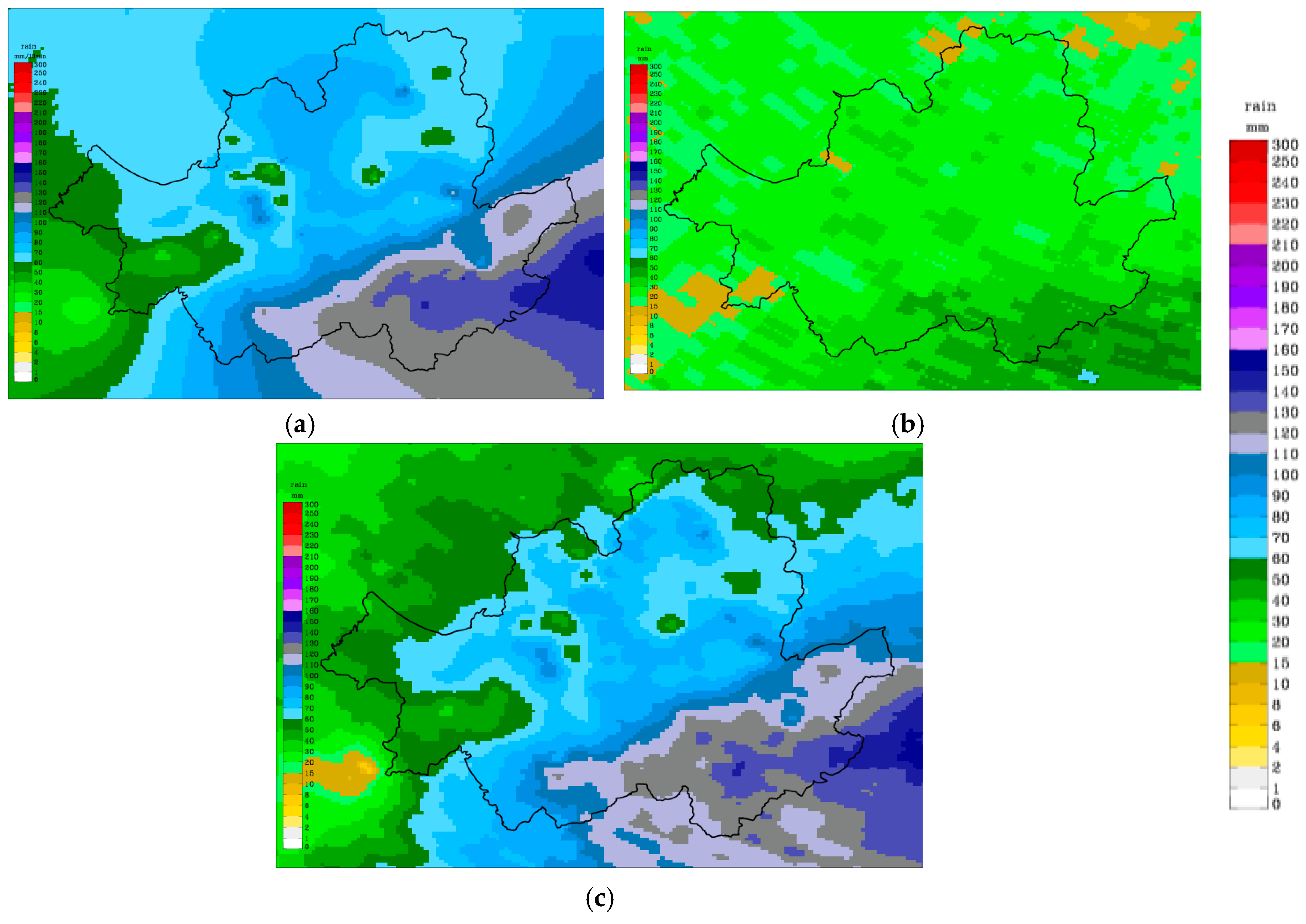
Figure 2 presents the results of using QPE products on 22 July 2013 (Case 3). Figure 2a shows QPE1, employing observed data from the 34 KMA AWSs and the 156 SKP AWSs by applying ordinary Kriging. As the figure shows, the central area of heavy rainfall was clearly identified in the southeast region of Seoul, although with more spatial fluctuations within the rainfall field. However, QPE1 shows a spatially smoothed pattern because the Kriging method is a least-error regression analysis method that can estimate a value with a tendency to have a minimized distribution at an unobserved point. Figure 2b shows QPE2, which was obtained by converting the reflectivity of the Gwangdeok weather radar to rainfall intensity with the Z = 200R1.6 equation. However, the amount of QPE3 rainfall is significantly different from the amount of observed rainfall from rain gauge stations. This underestimation occurred when the Marshall-Palmer equation was used, as this equation is normally used for stratiform precipitation in Korea. Figure 2c show the result of the conditional merging of the first two QPE products; in other words, QPE3 was generated by rainfall data from rain gauge networks of different densities and from weather radar. The estimated rainfall field of QPE3 appeared to adequately simulate the spatial irregularity of rainfall with a less smoothed pattern, while maintaining the quantity of rainfall close to that of the ground-observed rainfall. The results for the other three cases were similar to those of Case 3.
Figure 3 shows scatter plots of the ground-observed rainfall against each QPE product, which were constructed by randomly extracting data from gauge stations from data that was used for the cross validation of Case 2. Figure 3a shows the results of QPE1, in which the high-density gauge network was used. In this instance, the scatter plots showed a more dense distribution around the 45° (solid) line, indicating a small deviation from the validating gauge station. Figure 3b represents analyses of the Gwangdeok weather radar rainfall field (QPE2), in which the distributions occurred below the 45° line, indicating that the radar rainfall data were underestimated. The conditionally merged QPE3 results shown in Figure 3c also display a small deviation.
Table 2 shows a statistical assessment of the cross-validation analysis. The result shows that QPE2 had correlations between 0.49 and 0.77, RMSE values between 0.36 mm and 1.54 mm, and ME values between 0.08 mm and 0.32 mm when compared with ground-observed rainfall for four heavy rainfall events; all of these indicate a tendency to underestimate the four rainfall events. The MAE of QPE2 ranged from 0.07 mm to 0.44 mm and QPE2 showed the least accurate results when compared with the results of the other QPE products. For QPE1, the correlation ranged from 0.92 to 0.96 and RMSE ranged from 0.15 mm to 0.69 mm. The ME values were between 0.00 and 0.002 mm and the MAE ranged from 0.04 mm to 0.17 mm. For QPE3, the C-CORR ranged from 0.88 to 0.96, the RMSE values were between 0.20 mm and 0.72 mm, and the ME was −0.01 mm, indicating that QPE3 underestimated rainfall for the four events. The MAE of QPE3 was between 0.04 mm and 0.18 mm. QPE1 and QPE3 were quantitatively closer to the ground-observed rainfall than QPE2. Although the difference between QPE1 and QPE3 was small, the results of QPE1 were slightly superior to those of QPE3. The conditional merging method, which is used for QPE3 estimation with both rain gauges and radar, is very dependent on the rain gauge value in terms of quantitative rainfall amount. This is especially true at the rain gauge location when it used with data from very high density rain gauge networks. Therefore, the impact of radar data is very small.
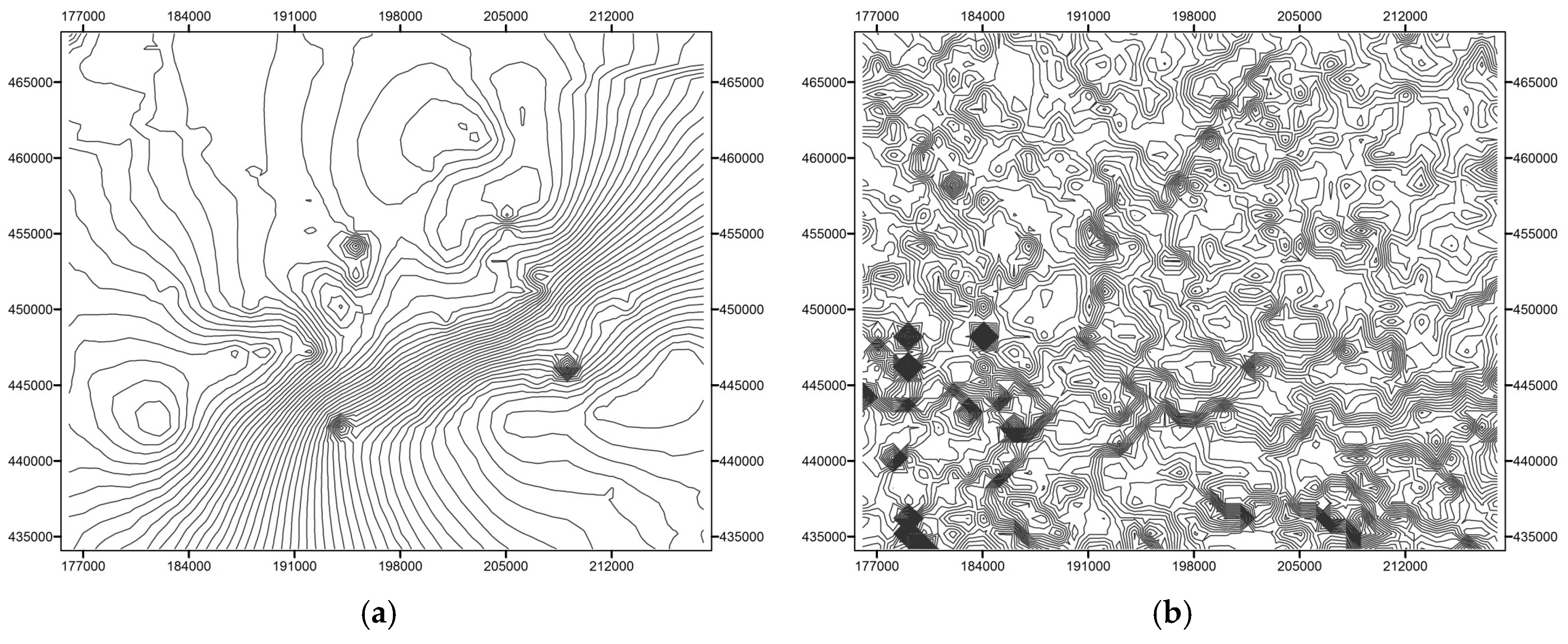
The estimated rainfall field is affected by the inaccuracy of radar QPEs when the rainfall field is conditionally merged. However, although the quantitative accuracy of QPE3 was lower than that of QPE1, QPE3 adequately simulated the irregularity of the spatial distribution. When considering this result, the spatial structure of rainfall was analyzed according to the contours of the QPEs. Figure 4 shows normalized rainfall contours that were derived from each accumulated QPE for 22 July 2013 (Case 3). This case had the largest coefficient of variation among all of the storm events. Accumulated rainfalls were normalized such that the spatial distribution could be confirmed without any absolute rainfall variation between QPEs; the contour interval was 0.02 mm. The general structure of the rainfall surface was substantially different than the contour of QPE1, which was estimated using only ground gauges. Figure 4a shows rainfall features that are smooth and circular with long lines. Figure 4b shows rainfall contours that are derived from radar data and the contours are very detailed. The contours of QPE3 feature much less smoothing than QPE1, but the rainfall distribution is not as detailed as QPE2. The spatial fluctuation of radar data was weakened because the quantitative rainfall error was compensated by the kriging field. However, it still shows that the irregularities in the rainfall distribution and the quantitative accuracy of radar rainfall were improved. The effect of the spatial distribution reproducibility of rainfall on hydrological simulations in the urban watershed with large spatial variations in rainfall is presented in Section 4.2.
To be used as an input to the hydrological model, the grid rainfall must be converted to MAP. For this purpose, the spatial variability of rainfall was confirmed in a small watershed of 7.4 km2 in Gangnam, while cross-validation was performed for the whole Seoul area (605 km2). The Gangnam area was then divided into 772 sub-basins, and the mean areal precipitation of each sub-basin was estimated using three types of QPEs. Two rain gauges (Gangnam and Seocho AWS), which were used for rainfall analysis in the study area before the installation of SKP stations, are used as a reference for this study (Figure 1b). The time series rainfall information from the Gangnam and Seocho rain gauge stations are shown in Figure 5 for all of the rainfall events. The observed rainfall data at these stations were similar for some events; however, the difference was 2 times for 10 min maximum rainfall and 1.5 times for 60 min maximum and total rainfall, although the distance between them was only 4123 m. Furthermore, the difference was observed even when peak rain occurred.
Subsequently, the spatial variation of mean areal rainfall was analyzed using a box-whisker plot. As shown in Figure 6, the range varied for each QPE type. Eighteen rain-gauge stations affected QPE1, and QPE2 was underestimated in comparison with the other QPE products. These analyses enabled the display of the difference and variability of rainfall within the sub-basin areas. As shown in the results of QPE1 and QPE3, the higher rain gauge density network provided wider variations for MAP estimation. Even though the basins are very small, large spatial differences of rainfall exist due to localized heavy rainfall. These results are in general agreement with previous experimental studies for the spatial variability of rainfall [38,39,40].
4.2. Urban Runoff Simulation with Various QPE Products
In this study, urban runoff simulations were performed using optimized parameters to confirm the effect of the QPE products. First, to optimize the parameters of the SWMM, water depth data were collected from a sewer pipe in July 2013. Water depth data, which are applicable to the target area, were observed at three water depth stations (22-0006, 22-0002, and 23-0006) at 1 min intervals using an ultrasonic sensor. Sewage from the Seocho 2 and Seocho 4 drainage districts passes through station 22-0002 and station 23-0006 is affected by the Yeoksam drainage district. Sewage from the Nonhyeon and Seocho 5 drainage districts passes through station 22-0006. The sewage passing through 22-0002 was combined with that passing through 23-0006 (Figure 1b). The initial depth of the combined sewer water was determined by the water depth using sewage data for each district per capita per day when there was no rainfall. The parameters (basin width, roughness coefficient, and curve number) of the SWMM model were determined by the measured water depth data and a trial and error method. The rainfall field of QPE1 was assumed to be the closest to the true value.
As shown in Figure 7, all rainfall data effectively simulated the peak water depth occurrence time and water depth change patterns. In addition, the simulation results were nearly the same when either QPE1 or QPE3 were used as input. However, as regards QPE2, in which the rainfall was underestimated, a significant reduction in the simulated sewer water depth was noted when compared with the other inputs of rainfall data.
Figure 8 and Table 3 show the evaluation results as the relative error of peak depth (REPD) and root mean square error (RMSE) for each simulation result using various QPE products for six rainfall events. The colored boxes in Figure 8 are drawn using the highest and lowest value of each statistic (RMSE, REPD) from each of the simulated QPF results. The applied events include Case 1 to Case 4, with the addition of Case 5 (2 July 2013) and Case 6 (4 July 2013). The average RMSE of QPE3 was the lowest (0.127 m), and the average RMSE of the Gangnam AWS was the highest (0.165 m). The average REPD of QPE3 (7.695%) was the lowest, followed by QPE1 (9.152%), Gangnam AWS (13.276%), Seocho AWS (16.331%), and QPE2 (56.792%). Figure 8 plots all of the evaluation results for these six storm events and three water depth observations. In the figure, the plot range of QPE3 is smaller than that of the other QPEs. As regards the runoff simulation results, the results of QPE3 were superior when compared with those of the other QPEs. QPE3 was slightly less accurate than QPE1 in the cross validation of rainfall analysis. However, the mean areal precipitation of the sub-basins using QPE3 combined with radar data showed better results for urban runoff simulation in terms of peak flow because QPE3 can provide the spatial description of rainfall for very small sub-basins, which is not produced by rain gauges.
This study analyzed the effect of QPE products by simulating the spatial runoff pattern in an urban area. The analysis was performed using observed inundation information for 22 July 2013, an event that caused actual inundation damage in the target area (side streets near the Gangnam subway station). The inundation information consists of digital photos that were taken at the inundation area and data from the National Disaster Management System (NDMS), such as information on inundated residences and buildings. No significant floods that were equivalent to those in 2010 or 2011 occurred in 2013; however, the NDMS confirmed inundation in buildings and roads. The white stars in Figure 9 indicate the locations of inundated areas. According to the NDMS, inundation depth reached more than 0.2 m. The circles in Figure 9 indicate the locations where the maximum simulated overflows occurred, which are color coded according to the type of QPE products. The black box and pentagon represent the locations of the maximum amount of overflow simulated using Seocho AWS and Gangnam AWS, respectively. The maximum overflow locations of QPE1, QPE3, and Gangnam AWS are very near the actual inundated area, but locations of other QPEs and Seocho AWS are quite distant from the actual inundated area. The size of circles, box, and pentagon represent the relative amount of the maximum overflow. The simulated node flooding results are summarized in Table 4.
For QPE2, the quantitative rainfall overflow was underestimated at only a few manholes; therefore, the flooding locations were quite few. The time series of overflows varied with the type of QPE product at flooding locations, as shown in Figure 10. The red graph lines of Figure 10 indicate the time series of overflows at the circles, box, and pentagon of Figure 9. The result of QPE3 appeared to be the most accurate in flow rate and overflow because QPE3 best estimated the spatial pattern of rainfall. In general, the simulated flows of each sub-basin area were affected by the spatial distribution of rainfall. Consequently, these results indicate that the use of high-resolution and highly accurate rainfall data is desirable in order to improve urban runoff analysis.
5. Conclusions
In this study, quality-controlled rainfall data from high-density ground-based rain-gauge networks covering Seoul, South Korea, were used with radar data to examine the estimations made by the QPE products at a resolution of 250 m and for urban runoff simulation. To examine the accuracy of the QPE products and for hydrological analysis, the data from the integrated meteorological sensors from the KMA and SKP were analyzed. A real-time quality control technique that can eliminate missing values and outliers was applied. The QPE products were used to make estimations based on four rainfall events that occurred in 2013. In addition, the three QPE products, which were classified according to the data used and the QPE method, were cross-validated. The quantitative accuracy of QPE2, which was only using weather radar data, was found to be underestimated when compared with the values that were derived from the ground gauge data. The accuracies of QPE1 and QPE3 were found to be good considering the rainfall amounts. Although the quantitative accuracy of QPE3 was lower than that of QPE1, QPE3 adequately simulated the irregularity of the spatial rainfall distribution. Each estimated QPE product was used for urban flood analysis and was tested for its applicability to urban flood analysis. In the evaluation of urban hydraulic and hydrologic impacts, according to three rainfall fields, QPE3, using both available rain gauges and radar data, simulated the peak runoff and overflow phenomena most accurately. This is because rainfall is generally non-homogeneous and QPE3 best reproduced spatial fluctuations of rainfall for small sub-basins. Therefore, urban runoff was reasonably simulated at the surface and in pipes. Hence, this study confirmed that spatial variations in rainfall and runoff can exist in a small urban area and that the use of high-resolution rainfall data is desirable for urban runoff analysis.
This study’s results show that radar data has few advantages over a sufficiently dense rain gauge network when estimating spatial rainfall distribution. However, the heterogeneity of the spatial distribution of rainfall can be better realized by radar; our results show that the accuracy of runoff analyses in urban watersheds is improved by this method. A radar will generally provide better quantitative precipitation estimates with a higher resolution, especially at the considered basin (30~50 km) in this study.
The limitation of this study lies in its generalization, as only a particular watershed was assessed for a few storm events. However, it is meaningful that the spatial variability of rainfall and the hydrological analysis of the urban watershed performed well using high density observation network and radar data for a wide urban area. In order to build on these results, future work should be conducted with more various storm events, and the errors should be corrected at each analysis step.
Acknowledgments
This study was funded by the Weather Information Service Engine (WISE) Program of the Korea Meteorological Administration under Grant KMIPA-2012-0001-1.
Author Contributions
Seong-Sim Yoon contributed to experiment, data analysis and draft and the revision of the manuscript. Byongju Lee contributed data analysis and revision of the manuscript.
Conflicts of Interest
The authors declare no conflict of interest.
References
- Yoon, D.K. Disaster and development examining global issues and cases. In Disaster Policies and Emergency Management in Korea; Kapucu, N., Liou, K.T., Eds.; Springer: Cham, Switzerland, 2014; pp. 149–164. [Google Scholar]
- Thorndahl, S.; Einfalt, T.; Wilems, P.; Nielsen, J.E.; Veldhuis, M.C.; Arnbjerg-Nielsen, K.; Rasmussen, M.R.; Molnar, P. Weather radar rainfall data in urban hydrology. Hydrol. Earth Syst. Sci. 2017, 21, 1359–1380. [Google Scholar] [CrossRef]
- Chen, D.; Ou, T.H.; Gong, L.B.; Xu, C.Y.; Li, W.J.; Ho, C.H.; Qian, W.H. Spatial interpolation of daily precipitation in China: 1951–2005. Adv. Atmos. Sci. 2010, 27, 1221–1232. [Google Scholar] [CrossRef]
- Michaud, J.D.; Sorooshian, S. Effect of rainfall-sampling errors on simulations of desert flash floods. Water Resour. Res. 1994, 30, 2765–2775. [Google Scholar] [CrossRef]
- Dong, X.; Dohmen-Janssen, C.M.; Booij, M.J. Appropriate spatial sampling of rainfall or flow simulation. Hydrol. Sci. J. 2005, 50, 279–298. [Google Scholar] [CrossRef]
- Srinivasan, G.; Nair, S. Daily rainfall characteristics from a high-density rain gauge network. Curr. Sci. 2005, 6, 942–946. [Google Scholar]
- Xu, H.; Xu, C.Y.; Chen, H.; Zhang, Z.; Li, L. Assessing the influence of rain gauge density and distribution on hydrological model performance in a humid region of China. J. Hydrol. 2013, 205, 1–12. [Google Scholar] [CrossRef]
- Vieux, B.; Vieux, J. Rainfall Accuracy Considerations Using Radar and Rain Gauge Networks for Rainfall-Runoff Monitoring. J. Water Manag. Model. 2005. [Google Scholar] [CrossRef]
- Schilling, W. Rainfall data for urban hydrology: What do we need? Atmos. Res. 1991, 27, 5–21. [Google Scholar] [CrossRef]
- Ochoa-Rodriguez, S.; Wang, L.P.; Gires, A.; Pina, R.D.; Reinoso-Rondinel, R.; Bruni, G.; Ichiba, A.; Gaitan, S.; Cristiano, E.; van Assel, J.; et al. Impact of spatial and temporal resolu tion of rainfall inputs on urban hydrodynamic modelling outputs: A multi-catchment investigation. J. Hydrol. 1995, 531, 389–407. [Google Scholar] [CrossRef]
- Sempere-Torres, D.; Corral, C.; Raso, J.; Malgrat, P. Use of weather radar of combined sewer overflows monitoring and control. J. Environ. Eng. 1999, 123, 372–380. [Google Scholar] [CrossRef]
- James, W.P.; Robinson, C.G.; Bell, J.F. Radar-assisted real-time flood forecasting. J. Water Resour. Plan. Manag. 1993, 119, 32–44. [Google Scholar] [CrossRef]
- Pessoa, M.L.; Rafael, L.B.; Earle, R.W. Use of weather radar for flood forecasting in the Sieve river basin: A sensitivity analysis. J. Appl. Meteorol. 1993, 32, 462–475. [Google Scholar] [CrossRef]
- Mimikou, M.A.; Baltas, E.A. Flood forecasting based on radar rainfall Measurements. J. Water Resour. Plan. Manag. 1996, 122, 151–156. [Google Scholar] [CrossRef]
- Sun, X.; Mein, R.G.; Keenan, T.D.; Elliott, J.F. Flood Estimation using Radar and Raingauge Data. J. Hydrol. 2000, 239, 4–18. [Google Scholar] [CrossRef]
- Kim, B.S.; Kim, B.K.; Kim, H.S. Flood simulation using the gauge-adjusted radar rainfall and physics-based distributed hydrologic model. Hydrol. Process. 2008, 22, 4400–4414. [Google Scholar]
- Krajewski, W.F. Cokriging radar-rainfall and rain gauge data. J. Geophys. Res. 1987, 92, 9571–9580. [Google Scholar] [CrossRef]
- Sinclair, S.; Pegram, G. Combining radar and rain gauge rainfall estimates using conditional merging. Atmos. Sci. Lett. 2005, 6, 19–22. [Google Scholar] [CrossRef]
- Seo, D.J.; Breidenbach, J.; Fulton, R.; Miller, D.; O’Bannon, T. Real-time adjustment of range dependent biases in WSR-88D rainfall estimates due to nonuniform vertical profile of reflectivity. J. Hydrometeorol. 2000, 1, 222–240. [Google Scholar] [CrossRef]
- Michelson, D.B. Quality Control of Weather Radar Data for Quantitative Application. Ph.D. Thesis, Telford Institute of Environmental Systems, University of Salford, Salford, UK, 2003. [Google Scholar]
- Liu, C.; Heckman, S. The application of the total lightning detection for severe storm prediction. In Proceedings of the WMO Technical Conference on Meteorological and Environmental Instruments and Methods of Observation (TECO-2010), Helsinki, Finland, 30 August–1 September 2010. [Google Scholar]
- Blumenfeld, K.A.; Skaggs, R.H. Using a high-density rain gauge network to estimate extreme rainfall frequencies in Minnesota. Appl. Geogr. 2011, 31, 5–11. [Google Scholar] [CrossRef]
- Tsuboya, H.; Kymagai, K.; Furuta, Y.; Miyajima, A. Environmental Sensor Network for NTT DOCOMO. J. Disaster Manag. 2016, 11, 334–339. [Google Scholar] [CrossRef]
- Korea Meteorological Agency. “Real-Time Quality Control System for Meteorological Gauged Data (I) Application.” 11-1360000-000206-01; Tech. Note 2006-2; Korea Meteorological Agency: Seoul, Korea, 2006; p. 157.
- Wade, C.G. A quality control program for surface mesometeorological data. J. Atmos. Ocean. Technol. 1987, 4, 435–453. [Google Scholar] [CrossRef]
- World Meteorological Organization (WMO). Guidelines on Quality Control Procedures for Data from Automatic Weather Stations; WMO: Geneva, Switzerland, 2004; p. 10. [Google Scholar]
- Heo, B.H.; Lee, J.A.; Chu, Y.O.; Kim, J.H.; Park, N.C.; Cho, J.Y.; Oh, S.J.; Noh, M.S.; Lee, Y.J. Statistical procedure of AWS gauged data to determine the threshold value for the RQMOD (real-time quality control system for meteorological gauged data). In Proceedings of the Autumn Meeting of Korean Meteorological Society, Seoul, Korea, 25 October 2005; pp. 390–391. [Google Scholar]
- Madsen, H. Semi-automatic Quality Control of Daily Precipitation Measurements. In Proceedings of the 5th International Meeting on Statistical Climatology, Toronto, ON, Canada, 22–26 June 1992; pp. 375–377. [Google Scholar]
- Madsen, H. Algorithms for correction of error types in a semi-automatic data collection. In Proceedings of the Precipitation Measurements and Quality Control: International Symposium on Precipitation and Evaporation, Bratislava, Slovakia, 20–24 September 1993; Sevruk, B., Lapin, M., Eds.; Slovak Hydrometeorological Institute: Bratislava, Slovakia, 1993. [Google Scholar]
- Yoon, S.S.; Lee, B.; Choi, Y. Deduction of Data Quality Control Strategy for High Density Rain Gauge Network in Seoul Area. J. Korea Water Resour. Assoc. 2015, 48, 245–255. (In Korean) [Google Scholar] [CrossRef]
- Mohr, C.G.; Vaughan, R.L. An economical procedure for Cartesian interpolation and display of reflectivity factor data in three-dimensional space. Bull. Am. Meteorol. Soc. 1979, 18, 661–670. [Google Scholar] [CrossRef]
- Goovaerts, P. Geostatistics for Natural Resources Evaluation, 4th ed.; Oxford University Press: New York, NY, USA, 2005. [Google Scholar]
- Yoon, S.S. Development of Optimal Radar Rainfall Estimation with Orographic Effect and Urban Flood Forecasting Application Technique. Ph.D. Thesis, Sejong University, Seoul, Korea, 2011. (In Korean). [Google Scholar]
- Deutsch, C.V.; Journel, A.G. GSLIB: Geostatistical Software Library and User’s Guide; Oxford University Press: New York, NY, USA, 1998. [Google Scholar]
- Yoon, S.S.; Bae, D.H. Optimal Rainfall Estimation by Considering Elevation at the Han River Basin, South Korea. J. Appl. Meteorol. Climatol. 2013, 52, 802–818. [Google Scholar] [CrossRef]
- Huber, W.C.; Heaney, J.P.; Nix, S.J.; Dickinson, R.E.; Polmann, D.J. Storm Water Management Model User’s Manuall Version III; US Environmental Protection Agency: Cininnati, OH, USA, 1984. [Google Scholar]
- Huber, W.C.; Dickinson, R.E. Storm Water Management Model, Version 4: User’s Manual; Environmental Research Laboratory, EPA: Athens, GA, USA, 1988. [Google Scholar]
- Jensen, N.E.; Pedersen, L. Spatial variablilty of rainfall: Variations within a single radar pixel. J. Atmos. Res. 2005, 77, 269–277. [Google Scholar] [CrossRef]
- Pedersen, L.; Jensen, N.E.; Christensen, L.E.; Madsen, H. Quantification of the spatial varibility of rainfall based on a dense network of rain gauges. Atmos. Res. 2010, 95, 441–454. [Google Scholar] [CrossRef]
- Tokay, A.; Roche, R.J.; Bashor, P.G. An Experimental study of spatial variability of rainfall. J. Hydrometeorol. 2014, 15, 801–812. [Google Scholar] [CrossRef]
Figure 1.
(a) The boundary of Seoul metropolitan area for which quantitative precipitation estimation (QPE) products were obtained and the study area rain gauge stations of the Korea Meteorological Administration (KMA) (black stars) and SK Planet (red circles); (b) drainage system and observation stations of rain and water depth (black triangles).
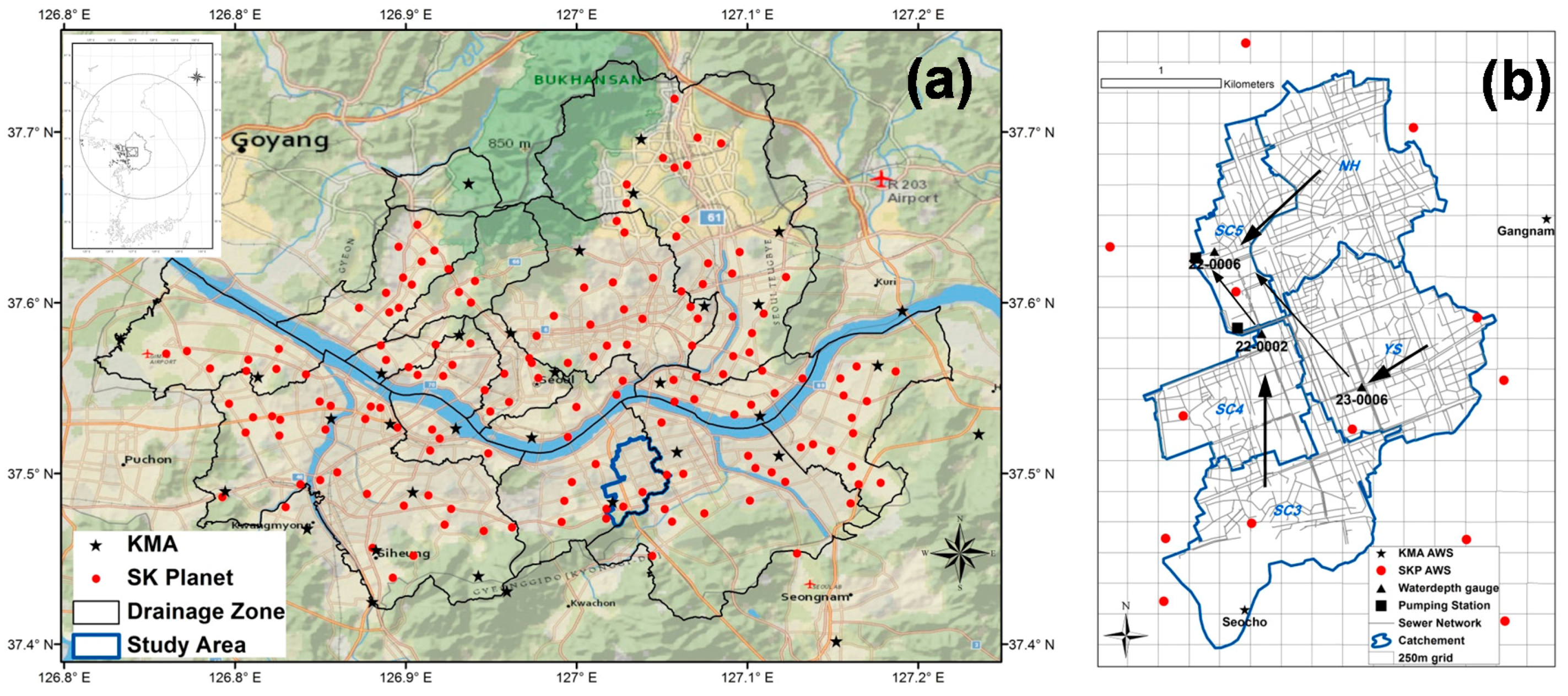
Figure 2.
Accumulated rainfall distribution determined on 22 July 2013 using quantitative precipitation estimation methods: (a) QPE 1; (b) QPE 2; (c) QPE 3.
Figure 2.
Accumulated rainfall distribution determined on 22 July 2013 using quantitative precipitation estimation methods: (a) QPE 1; (b) QPE 2; (c) QPE 3.

Figure 3.
Scatter diagrams of three quantitative precipitation estimation products by cross validation for 22 July 2013: (a) QPE 1; (b) QPE 2; (c) QPE 3.
Figure 3.
Scatter diagrams of three quantitative precipitation estimation products by cross validation for 22 July 2013: (a) QPE 1; (b) QPE 2; (c) QPE 3.
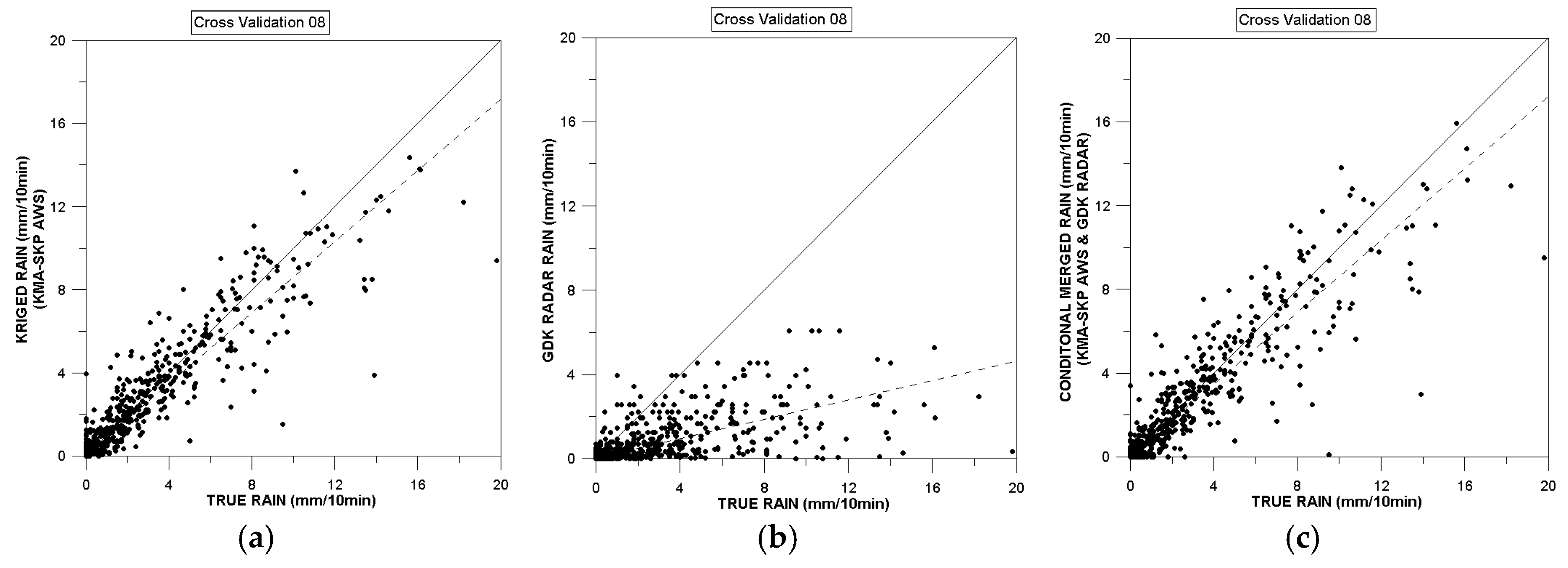
Figure 4.
Normalized rainfall contours for 22 July 2013: (a) Rainfall contours derived from QPE1; (b) Rainfall contours derived from QPE2; (c) Rainfall contours derived from QPE3.
Figure 4.
Normalized rainfall contours for 22 July 2013: (a) Rainfall contours derived from QPE1; (b) Rainfall contours derived from QPE2; (c) Rainfall contours derived from QPE3.

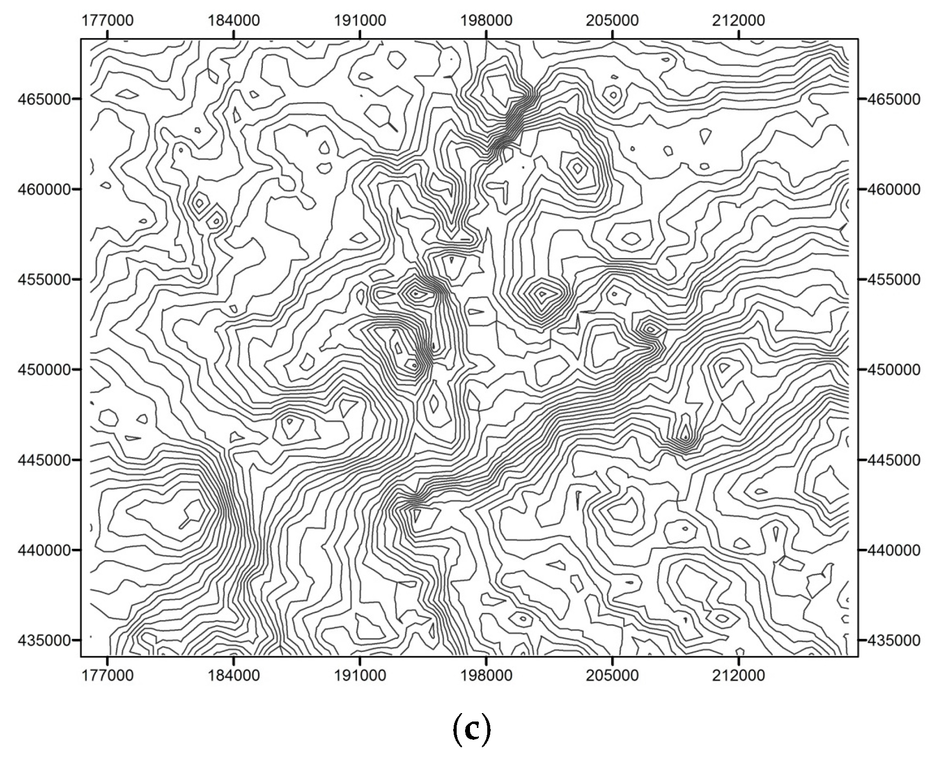
Figure 5.
Time series rainfall information for all of the rainfall events.
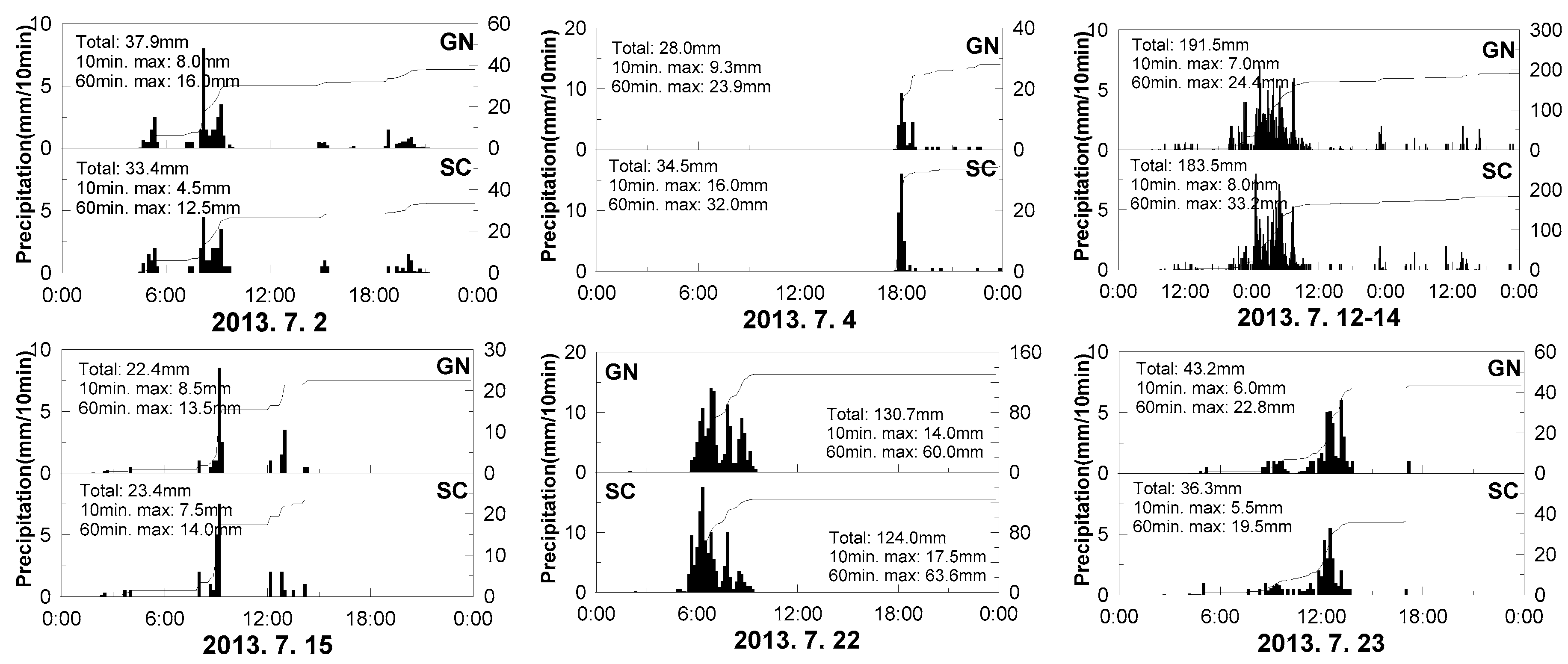
Figure 6.
Distribution of Mean Areal Precipitation for 772 sub-basins: (a) 2 July 2013; (b) 4 July 2013; (c) 12–14 July 2013; (d) 15 July 2013; (e) 22 July 2013; (f) 23 July 2013.
Figure 6.
Distribution of Mean Areal Precipitation for 772 sub-basins: (a) 2 July 2013; (b) 4 July 2013; (c) 12–14 July 2013; (d) 15 July 2013; (e) 22 July 2013; (f) 23 July 2013.
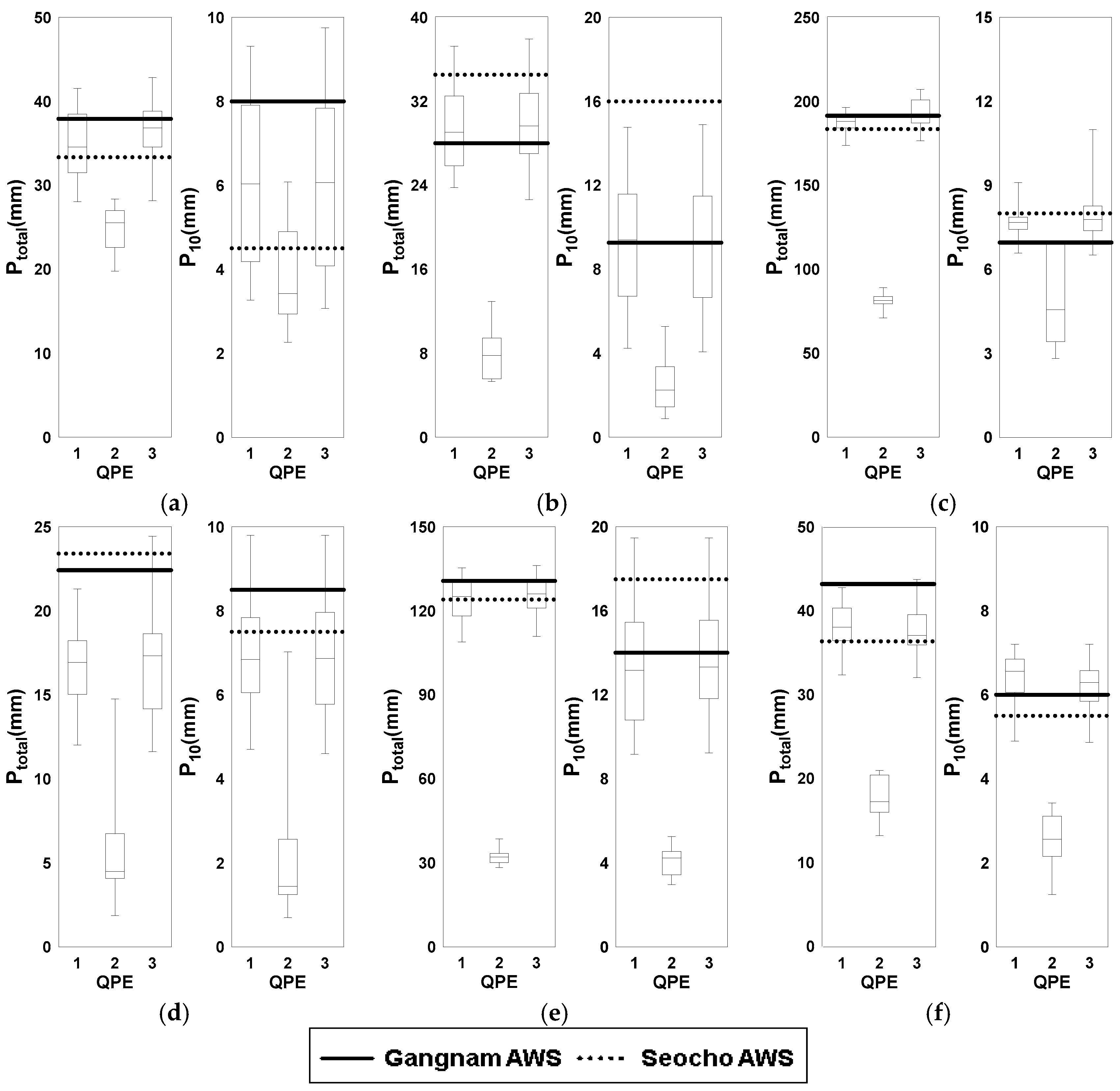
Figure 7.
Comparisons between observed and simulated depths in manholes: (a) 2 July 2013; (b) 4 July 2013; (c) 12–14 July 2013; (d) 15 July 2013; (e) 22 July 2013; (f) 23 July 2013.
Figure 7.
Comparisons between observed and simulated depths in manholes: (a) 2 July 2013; (b) 4 July 2013; (c) 12–14 July 2013; (d) 15 July 2013; (e) 22 July 2013; (f) 23 July 2013.
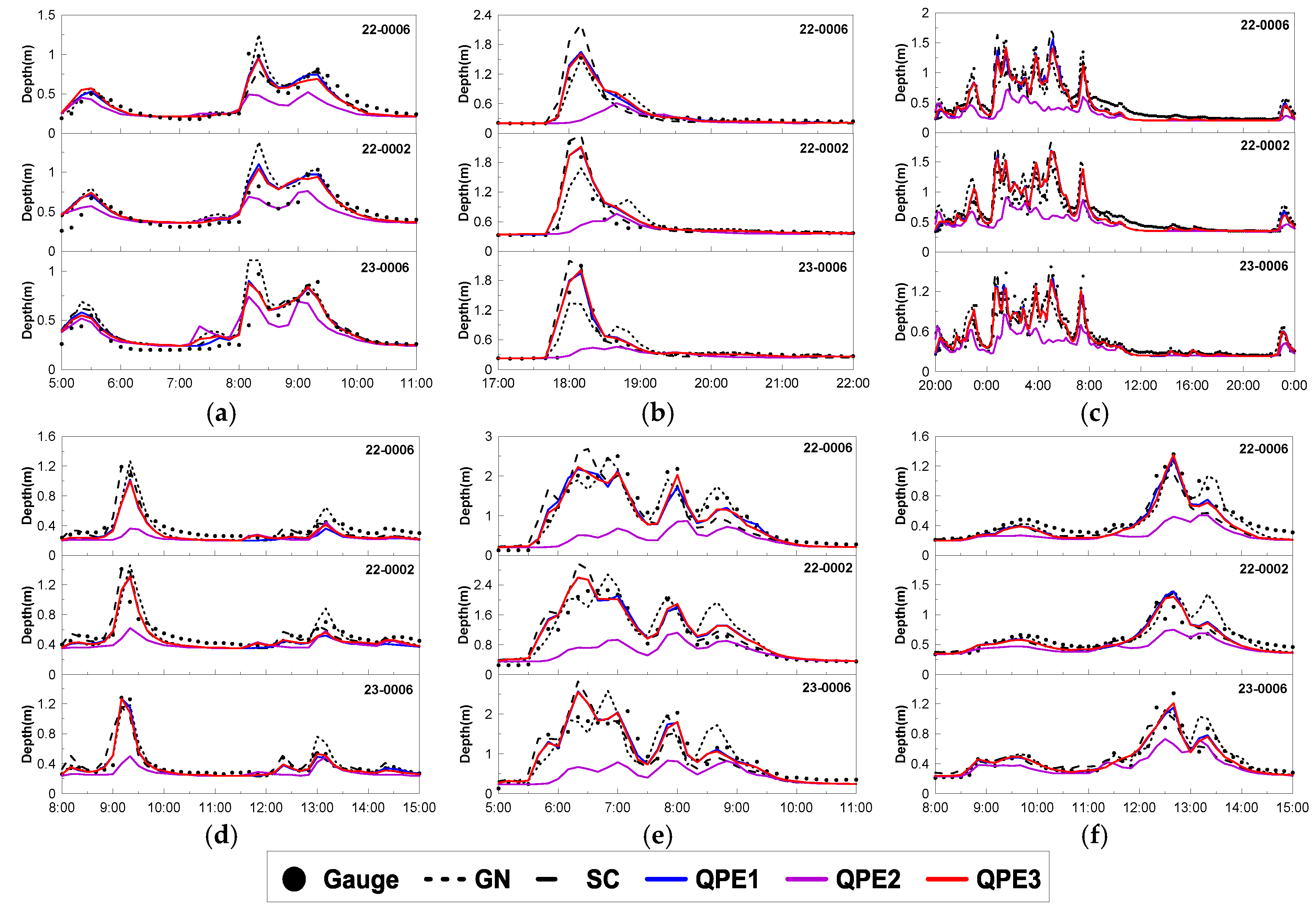
Figure 8.
Evaluation results in terms of relative error of peak depth (REPD) and root mean square error (RMSE) for simulated depth using various QPE products.
Figure 8.
Evaluation results in terms of relative error of peak depth (REPD) and root mean square error (RMSE) for simulated depth using various QPE products.
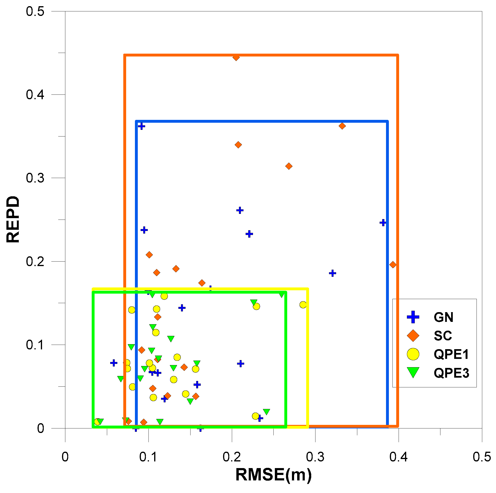
Figure 9.
Locations where real flooding occurred and locations of maximum simulated total flood volume according to the type of QPE product.
Figure 9.
Locations where real flooding occurred and locations of maximum simulated total flood volume according to the type of QPE product.
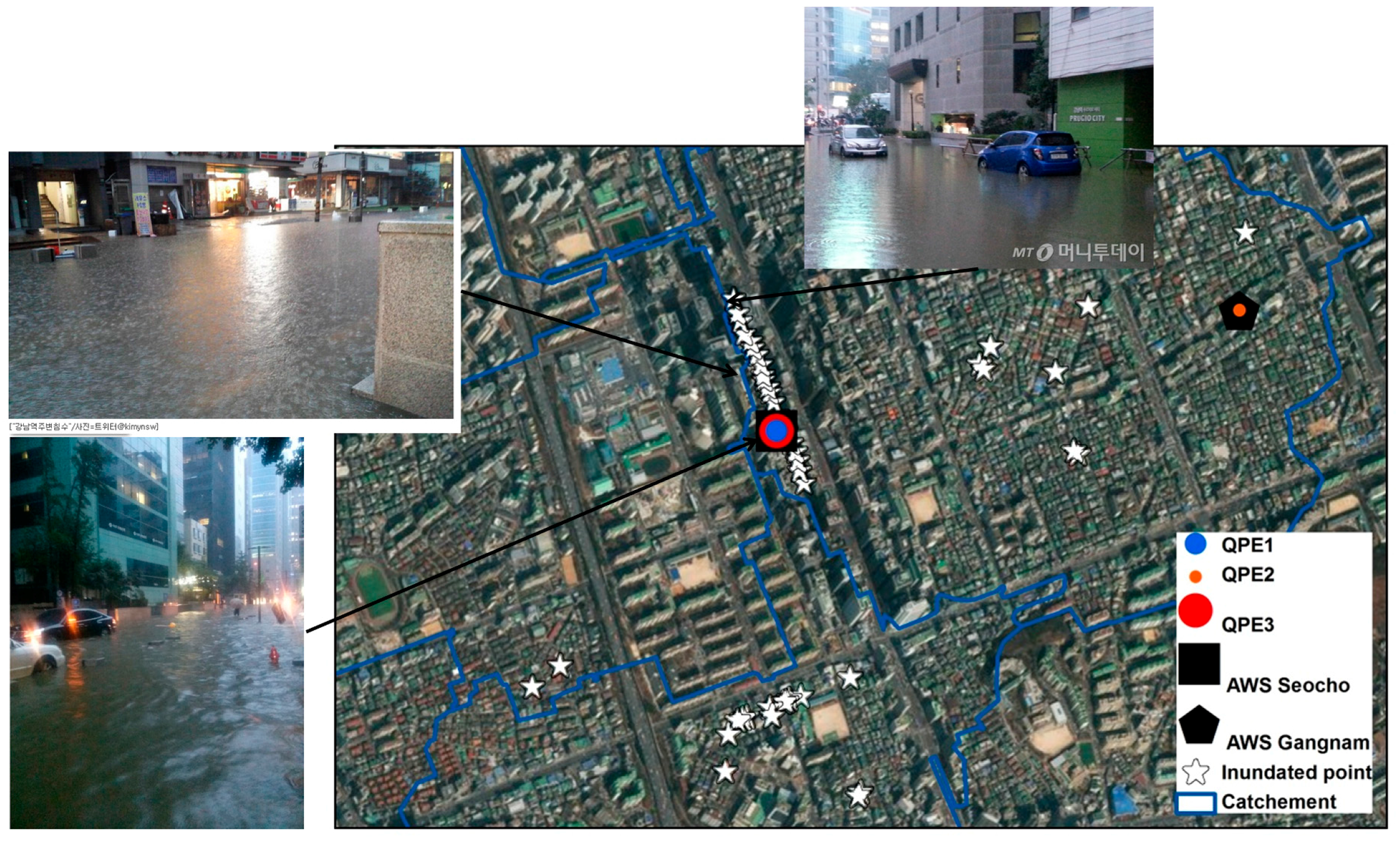
Figure 10.
Timeseries overflow of each QPEs at all flooding occurred locations.


Table 1.
Criteria of missing and outlier data.
| Status | Criteria |
|---|---|
| Missing value | Recorded observation data as “NULL” value |
| Outlier |
|
Table 2.
Statistics of the comparison between the cross-validation estimates of each quantitative precipitation estimations and rain gauge observations.
Table 2.
Statistics of the comparison between the cross-validation estimates of each quantitative precipitation estimations and rain gauge observations.
| Event | Item | Test Stations | QPE1 | QPE2 | QPE3 |
|---|---|---|---|---|---|
| Case 1 | Total rainfall | 4174.221 | 4186.78 | 1653.51 | 4024.08 |
| C-CORR | - | 0.95 | 0.66 | 0.94 | |
| RMSE (mm) | - | 0.34 | 0.91 | 0.37 | |
| ME (mm) | - | 0.001 | −0.23 | −0.01 | |
| MAE (mm) | - | 0.10 | 0.29 | 0.11 | |
| Case 2 | Total rainfall | 193.38 | 197.77 | 72.07 | 159.52 |
| C-CORR | - | 0.92 | 0.49 | 0.88 | |
| RMSE (mm) | - | 0.15 | 0.36 | 0.20 | |
| ME (mm) | - | 0.002 | −0.04 | −0.01 | |
| MAE (mm) | - | 0.04 | 0.07 | 0.04 | |
| Case 3 | Total rainfall | 1647.38 | 1635.78 | 519.06 | 1606.39 |
| C-CORR | - | 0.93 | 0.73 | 0.93 | |
| RMSE (mm) | - | 0.69 | 1.54 | 0.72 | |
| ME (mm) | - | 0.001 | −0.41 | −0.01 | |
| MAE (mm) | - | 0.17 | 0.44 | 0.18 | |
| Case 4 | Total rainfall | 910.85 | 909.08 | 331.17 | 877.06 |
| C-CORR | - | 0.96 | 0.77 | 0.96 | |
| RMSE (mm) | - | 0.29 | 0.84 | 0.31 | |
| ME (mm) | - | −0.0006 | −0.21 | −0.01 | |
| MAE (mm) | - | 0.08 | 0.23 | 0.09 |
Table 3.
Evaluation results in terms of REPD and RMSE for simulated water depth using various QPE products.
Table 3.
Evaluation results in terms of REPD and RMSE for simulated water depth using various QPE products.
| Rainfall Type | GN | SC | QPE1 | QPE2 | QPE3 | ||||||
|---|---|---|---|---|---|---|---|---|---|---|---|
| Event | Station | RMSE (mm) | REPD (%) | RMSE (mm) | REPD (%) | RMSE (mm) | REPD (%) | RMSE (mm) | REPD (%) | RMSE (mm) | REPD (%) |
| Case 1 | 22-0006 | 0.16 | 5.23 | 0.21 | 33.99 | 0.13 | 8.50 | 0.44 | 52.94 | 0.13 | 7.19 |
| 22-0002 | 0.21 | 7.74 | 0.16 | 17.42 | 0.16 | 7.10 | 0.31 | 60.65 | 0.16 | 7.74 | |
| 23-0006 | 0.21 | 26.12 | 0.16 | 3.82 | 0.11 | 11.47 | 0.36 | 69.43 | 0.11 | 12.10 | |
| Case 2 | 22-0006 | 0.10 | 6.72 | 0.08 | 0.84 | 0.11 | 14.29 | 0.20 | 69.75 | 0.10 | 15.97 |
| 22-0002 | 0.12 | 3.55 | 0.09 | 0.71 | 0.10 | 7.80 | 0.18 | 56.03 | 0.10 | 7.09 | |
| 23-0006 | 0.06 | 7.81 | 0.09 | 9.38 | 0.04 | 0.78 | 0.18 | 60.94 | 0.04 | 0.78 | |
| Case 3 | 22-0006 | 0.23 | 1.20 | 0.39 | 19.60 | 0.31 | 25.60 | 0.88 | 72.80 | 0.26 | 16.00 |
| 22-0002 | 0.32 | 18.58 | 0.27 | 31.42 | 0.23 | 15.04 | 0.66 | 68.14 | 0.23 | 15.04 | |
| 23-0006 | 0.38 | 24.64 | 0.33 | 36.23 | 0.23 | 3.38 | 0.69 | 61.84 | 0.24 | 1.93 | |
| Case 4 | 22-0006 | 0.11 | 6.62 | 0.13 | 19.12 | 0.11 | 3.68 | 0.27 | 61.77 | 0.11 | 0.74 |
| 22-0002 | 0.17 | 16.67 | 0.11 | 13.33 | 0.12 | 15.83 | 0.17 | 37.50 | 0.11 | 8.33 | |
| 23-0006 | 0.10 | 16.42 | 0.11 | 18.66 | 0.08 | 14.18 | 0.16 | 45.52 | 0.08 | 9.70 | |
| Case 5 | 22-0006 | 0.10 | 23.76 | 0.10 | 20.79 | 0.08 | 4.95 | 0.18 | 51.49 | 0.09 | 5.94 |
| 22-0002 | 0.16 | 0.00 | 0.12 | 3.88 | 0.13 | 5.83 | 0.13 | 26.21 | 0.13 | 10.68 | |
| 23-0006 | 0.14 | 14.43 | 0.11 | 8.25 | 0.11 | 7.22 | 0.14 | 23.71 | 0.10 | 9.28 | |
| Case 6 | 22-0006 | 0.09 | 0.00 | 0.21 | 44.44 | 0.07 | 7.84 | 0.32 | 60.13 | 0.07 | 5.88 |
| 22-0002 | 0.22 | 23.29 | 0.14 | 7.31 | 0.14 | 4.11 | 0.42 | 65.30 | 0.15 | 3.20 | |
| 23-0006 | 0.09 | 36.19 | 0.11 | 4.76 | 0.07 | 7.14 | 0.19 | 78.10 | 0.07 | 0.92 | |
| Average | 0.165 | 13.276 | 0.162 | 16.331 | 0.129 | 9.152 | 0.327 | 56.792 | 0.127 | 7.695 | |
Table 4.
Simulated node flooding results using Storm Water Management Model (SWMM) for 22 July 2013.
Table 4.
Simulated node flooding results using Storm Water Management Model (SWMM) for 22 July 2013.
| Item | GN | SC | QPE1 | QPE2 | QPE3 |
|---|---|---|---|---|---|
| No. of Flooded Nodes | 29 | 71 | 33 | 1 | 38 |
| Hours Flooded | 2.38 | 2.12 | 2.56 | 0.16 | 2.57 |
| Maximum Rate (CMS) | 13.00 | 25.75 | 14.88 | 0.33 | 15.31 |
| Total Flood Volume (106 Ltr) | 22.07 | 34.89 | 25.52 | 0.10 | 25.14 |
© 2017 by the authors. Licensee MDPI, Basel, Switzerland. This article is an open access article distributed under the terms and conditions of the Creative Commons Attribution (CC BY) license (http://creativecommons.org/licenses/by/4.0/).
Share and Cite
MDPI and ACS Style
Yoon, S.-S.; Lee, B. Effects of Using High-Density Rain Gauge Networks and Weather Radar Data on Urban Hydrological Analyses. Water 2017, 9, 931. https://doi.org/10.3390/w9120931
AMA Style
Yoon S-S, Lee B. Effects of Using High-Density Rain Gauge Networks and Weather Radar Data on Urban Hydrological Analyses. Water. 2017; 9(12):931. https://doi.org/10.3390/w9120931
Chicago/Turabian StyleYoon, Seong-Sim, and Byongju Lee. 2017. "Effects of Using High-Density Rain Gauge Networks and Weather Radar Data on Urban Hydrological Analyses" Water 9, no. 12: 931. https://doi.org/10.3390/w9120931
Note that from the first issue of 2016, this journal uses article numbers instead of page numbers. See further details here.