A Statistical Method to Predict Flow Permanence in Dryland Streams from Time Series of Stream Temperature
by
 , ,
, ,
Ivan Arismendi
1,* ,
,
Jason B. Dunham
2,
Michael P. Heck
2,
Luke D. Schultz
2,3 and
David Hockman-Wert
2 1
Department of Fisheries and Wildlife, Oregon State University, 104 Nash Hall, Corvallis, OR 97331, USA
2
U.S. Geological Survey, Forest and Rangeland Ecosystem Science Center, 3200 SW Jefferson Way, Corvallis, OR 97331, USA
3
Wyoming Game and Fish Department, P.O. Box 850, Pinedale, WY 82941, USA
*
Author to whom correspondence should be addressed.
Water 2017, 9(12), 946; https://doi.org/10.3390/w9120946
Submission received: 12 October 2017
/
Revised: 30 November 2017
/
Accepted: 1 December 2017
/
Published: 5 December 2017
Abstract
:Intermittent and ephemeral streams represent more than half of the length of the global river network. Dryland freshwater ecosystems are especially vulnerable to changes in human-related water uses as well as shifts in terrestrial climates. Yet, the description and quantification of patterns of flow permanence in these systems is challenging mostly due to difficulties in instrumentation. Here, we took advantage of existing stream temperature datasets in dryland streams in the northwest Great Basin desert, USA, to extract critical information on climate-sensitive patterns of flow permanence. We used a signal detection technique, Hidden Markov Models (HMMs), to extract information from daily time series of stream temperature to diagnose patterns of stream drying. Specifically, we applied HMMs to time series of daily standard deviation (SD) of stream temperature (i.e., dry stream channels typically display highly variable daily temperature records compared to wet stream channels) between April and August (2015–2016). We used information from paired stream and air temperature data loggers as well as co-located stream temperature data loggers with electrical resistors as confirmatory sources of the timing of stream drying. We expanded our approach to an entire stream network to illustrate the utility of the method to detect patterns of flow permanence over a broader spatial extent. We successfully identified and separated signals characteristic of wet and dry stream conditions and their shifts over time. Most of our study sites within the entire stream network exhibited a single state over the entire season (80%), but a portion of them showed one or more shifts among states (17%). We provide recommendations to use this approach based on a series of simple steps. Our findings illustrate a successful method that can be used to rigorously quantify flow permanence regimes in streams using existing records of stream temperature.
1. Introduction
Perhaps one of the most fundamental issues concerning flow permanence in stream channels is the lack of understanding about expected spatial and temporal patterns across landscapes, riverscapes, or stream networks [1,2]. Many studies, ranging from work conducted in the 1950s [3] to more contemporary assessments [4,5], consistently point to inaccuracies in characterization of flow permanence on existing maps. Efforts to improve quantification of flow permanence in the field have involved a host of techniques ranging from direct observation to various forms of instrumentation [6,7]. Among these, indirect quantification of flow permanence via time series of temperature recorded in stream channels is particularly promising. These instrumental records are already available in many regions, often comprising datasets consisting of thousands of individually monitored sites [8]. In practice, stream temperature records that indicate a dry stream channel are often edited or deleted, without considering the value of such information in diagnosing drying.
As a first step to diagnosing drying, Sowder and Steel [9] recommend several automatable checks that allow users to flag potentially aberrant time periods from these time series, followed by visual inspection of the flagged temperature records. Because the specific heat of water is over four times that of air, data loggers in dry stream channels typically display highly variable daily temperature records [10,11]. Secondly, Sowder and Steel [9] recommend examining paired water and air temperature records for a given site, if available.
In this study, we build on prior work to apply a more formal statistical method, Hidden Markov Models (HMMs) [12], to diagnose patterns of stream drying from hourly records of stream temperatures. We first applied HMMs to a selection of sites with paired air and in-channel temperature recordings to compare daily variability in each [9,10] and illustrate how HMMs can allow for more objective identification of transitions between wet and dry states in stream channels. Next, we used information from pairs of in-channel temperature data loggers and electrical resistors that instantaneously detect loss (or gain) of flows [13]. This allowed us to compare results of statistical analyses with known measurements of flow permanence at selected sites. Finally, we applied HMMs across a full network of locations monitored within a large watershed [14] to illustrate patterns in the timing, duration, and frequency of flow permanence in the system [1]. Collectively, these results illustrate a new and readily applied method that can be used to rigorously quantify stream flow permanence regimes from existing records of stream temperature. This may be relevant to assess responses of flow permanence to a host of potential influences, including changing climatic conditions and the effects of land and water uses [1,5].
2. Materials and Methods
2.1. Field Data Collection
We collected stream temperature, air temperature, and flow permanence data from two regions in the northern Great Basin: the Willow and Whitehorse Creek watershed (WWC) of southeast Oregon and the Willow and Rock Creek watershed of north-central Nevada (WRC; Figure 1). The number of data loggers and their distribution within each watershed was driven by objectives from previous studies [14] and thus, an ideal configuration of paired air and stream data loggers at WRC and paired electrical resistors and stream data loggers at WWC was not possible. However, our comparisons are valid and useful for the purposes here. Field data collection followed protocols described by Heck et al. [15] and Schultz et al. [14]. Stream and air temperature measurements were recorded hourly with HOBO U-22 (Onset Computer Corporation, Bourne, MA, USA) waterproof temperature data loggers. In WWC, stream temperatures were tracked at hourly intervals between 1 April and 27 August 2015. At eight sites, we co-located stream temperature data loggers with electrical resistors to track patterns of drying [13]. Electrical resistors were constructed following methods described by Chapin et al. [16]. Furthermore, hourly stream temperature recordings were paired with air temperature recordings at eight locations in WRC from 1 April through 27 July 2016. Lastly, we used stream temperature data from 102 data loggers located throughout the WWC to apply our statistical analysis (see below) across the full network.
2.2. Statistical Analyses
Hidden Markov Models (HMMs) [12,17] can be used to represent stochastic processes (i.e., whether a data logger is underwater) with an a priori set of discrete states (i.e., dry or wet) and probabilistic transitions between them. To illustrate this, consider a stream reach in the wet state on day 1. On day 2, there could be a 90% chance of staying in the same state and 10% chance of moving to the dry state. Similarly, if the stream reach is in the dry state on day 1, there is a chance to stay in the same state, but also a chance to move to the wet state on day 2. The Markov portion of the HMMs refers to the time dependence of observations as the current state depends on the previous state [17], but the true underlying states of the model are hidden and cannot be observed directly. Thus, the resulting distribution function is not deterministic, but rather a probability density distribution given the observed data [17]. HMMs can be used to determine the state transition probabilities that underlie the stochastic process in question as well as the distributional parameters for each state [18]. These calculations are computationally intensive due to the estimation of the likelihood and posterior state sequence of the HMM. Visser [17] provides a detailed discussion about the different approaches and alternative algorithms existing to computationally solve these issues. In our study, we adapted the R-code provided by Visser [17] for the 2-state mixture model using the package depmixS4 [18] in R [19].
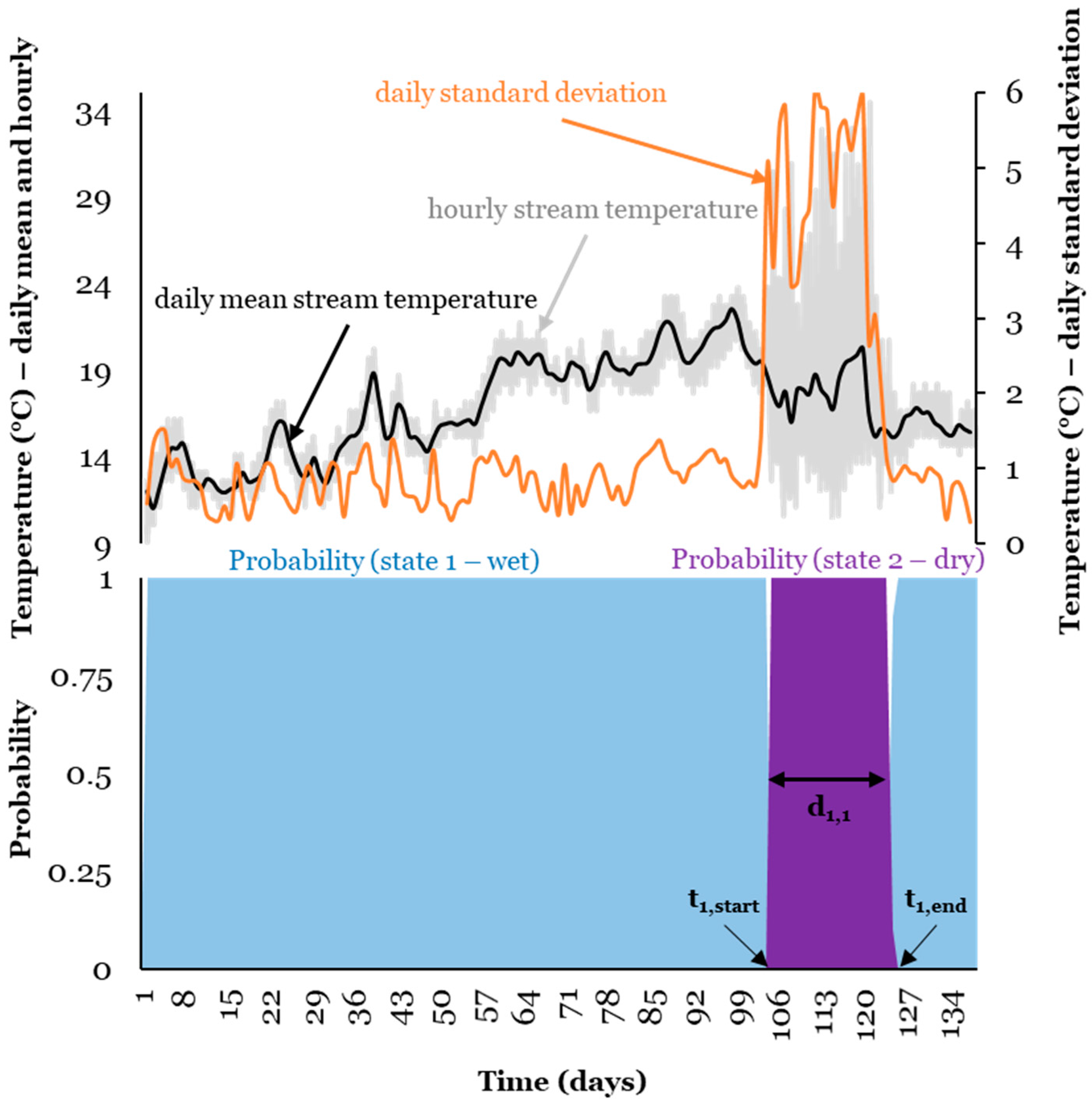
We initially considered several descriptors of daily stream temperature to be included as time series to diagnose stream drying using HMMs (Figure 2). We evaluated potential time series that contained both wet and dry states from a subset of time series and identified the daily standard deviation (SD, a measure of variability in hourly recorded temperatures within a day) as the most appropriate metric to be used in the HMM. Because water has a much higher specific heat compared to air, we expected that under wet conditions, diel fluctuations in temperature would be reduced compared to dry conditions and thus, display a smaller daily SD. We used the subset of sites that contained electrical resistors from WWC and paired air–water data loggers from the WRC to crosscheck our predictions about timing of wet and dry states.
Our analyses focused on capturing changes in states during spring/summer and therefore we used time series data between April and August. When applying HMMs to these time series, the HMM algorithm forced the data to detect two states from the wet and dry signals. However, in cases when stream reaches stayed dry or had permanent water during the entire time period (i.e., single state), the HMMs still forced the identification of two states. These detected state changes were most likely due to short-term local hydroclimatic influences and not necessarily associated with purely wet and dry conditions. In such cases, we used additional information from time series of air temperature (i.e., when the maximum daily stream temperature was similar or different to the maximum daily air temperature) and electrical resistors (i.e., readings >0 or <0) to deduce if the detected changes in state were or were not associated with shifts between wet and dry conditions. A detailed review of the time series showed that, as a conservative rule of thumb, when the HMM identified more than seven changes among states they were not due to a shift between wet and dry conditions, but rather a single constant state over the entire time (wet or dry). We applied this procedure to all time series of stream temperature from WWC to illustrate patterns in the timing, duration, and frequency of flow permanence within an entire stream network.
3. Results
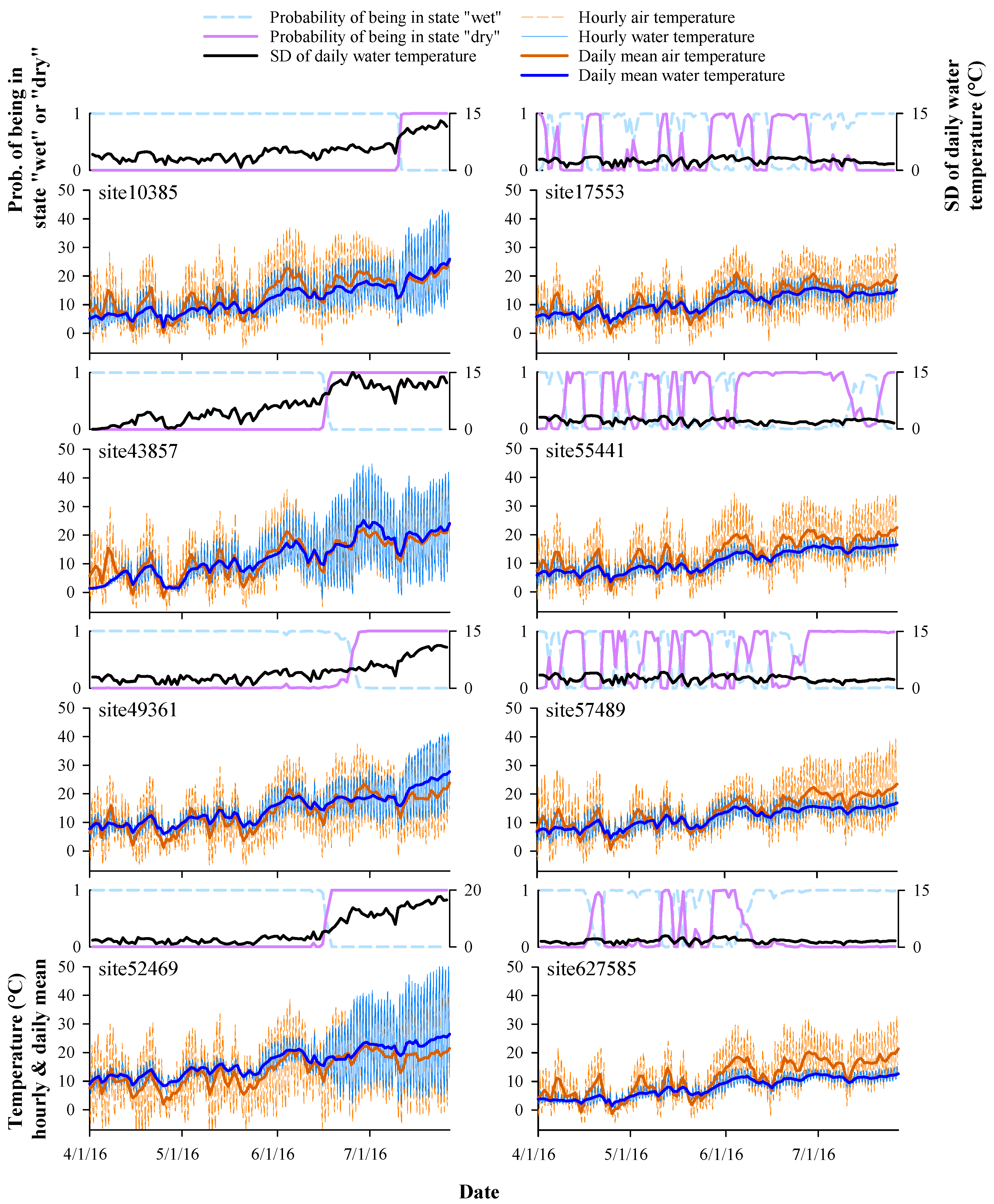
HMMs applied to time series of daily SD of stream temperatures successfully identified and separated signals from wet and dry conditions of stream reaches when paired stream and air temperature data loggers were examined at WRC during the period 1 April–27 July 2016 (Figure 3). The use of HMMs allowed us to identify what visually appeared to be both dry and wet states as well as their shifts over time. At WRC, we found patterns of wet–dry (e.g., site10385, site43857, site49361 and site52469), and purely wet states (e.g., site17553, site55441, site57489 and site627585). The use of HMMs was also effective in identifying shifts in timing between dry and wet states when sites went dry at different times (e.g., site10385 versus site43857 and site52469). The timing and type of state identified by each HMM closely tracked visual convergence of daily SD in stream channels and air temperatures as channels dried. In cases when the HMM identified a single wet state, contrasting hourly time series of stream and air temperature (i.e., site17553, site55441, site57489 and site627585) also provided visual corroboration.
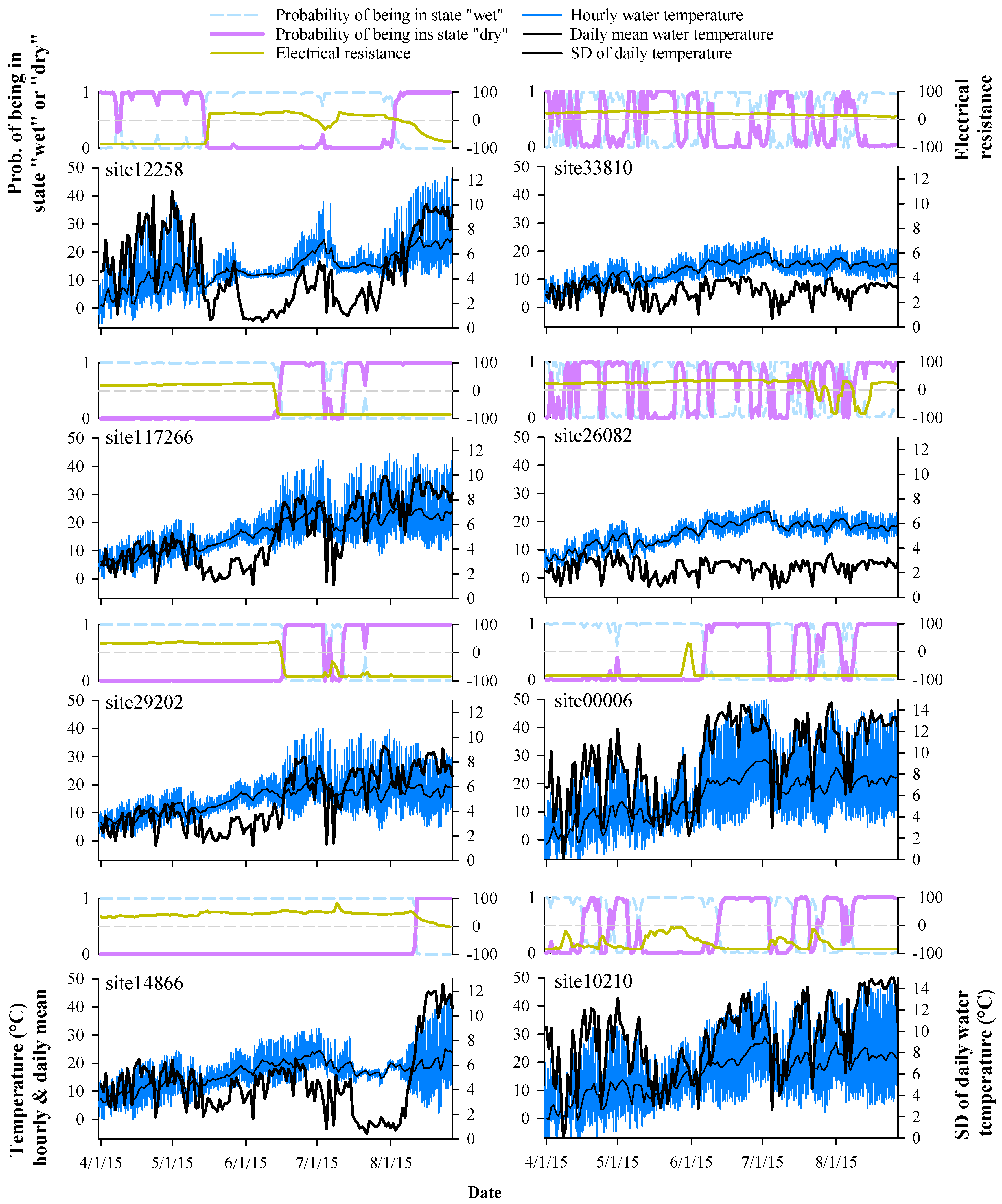
Pairing of electrical resistors and stream temperature data loggers in WWC provided confirmation of drying in the field and opportunities to evaluate how HMMs diagnosed drying based on daily SD of stream temperatures (Figure 4). The timing of drying, if a site experienced drying, was indicated by negative values recorded by the electrical resistors (positive values represented wet conditions). Time series of daily SD of stream temperature used as inputs for HMMs extended from 1 April to 27 August 2015. Among the eight sites with paired electrical resistors, we identified four patterns of change, including dry–wet–dry (e.g., site12258), wet–dry (e.g., site117266, site29202, and site14866), continuously wet (e.g., site33810, site26082) and continuously dry (e.g., site00006, site10210). The use of HMMs was effective in diagnosing all of these cases, regardless of the timing of shifts between states or degree of synchrony (timing of changes in states) among them (e.g., site117266 and site29202 versus site14866). In cases when the HMM identified a single state (dry or wet) occurring during the entire time period, we used a second source of information (hourly stream temperature) to visually confirm and separate between a single wet (site33810, site26082) and a single dry state (site00006, site10210).
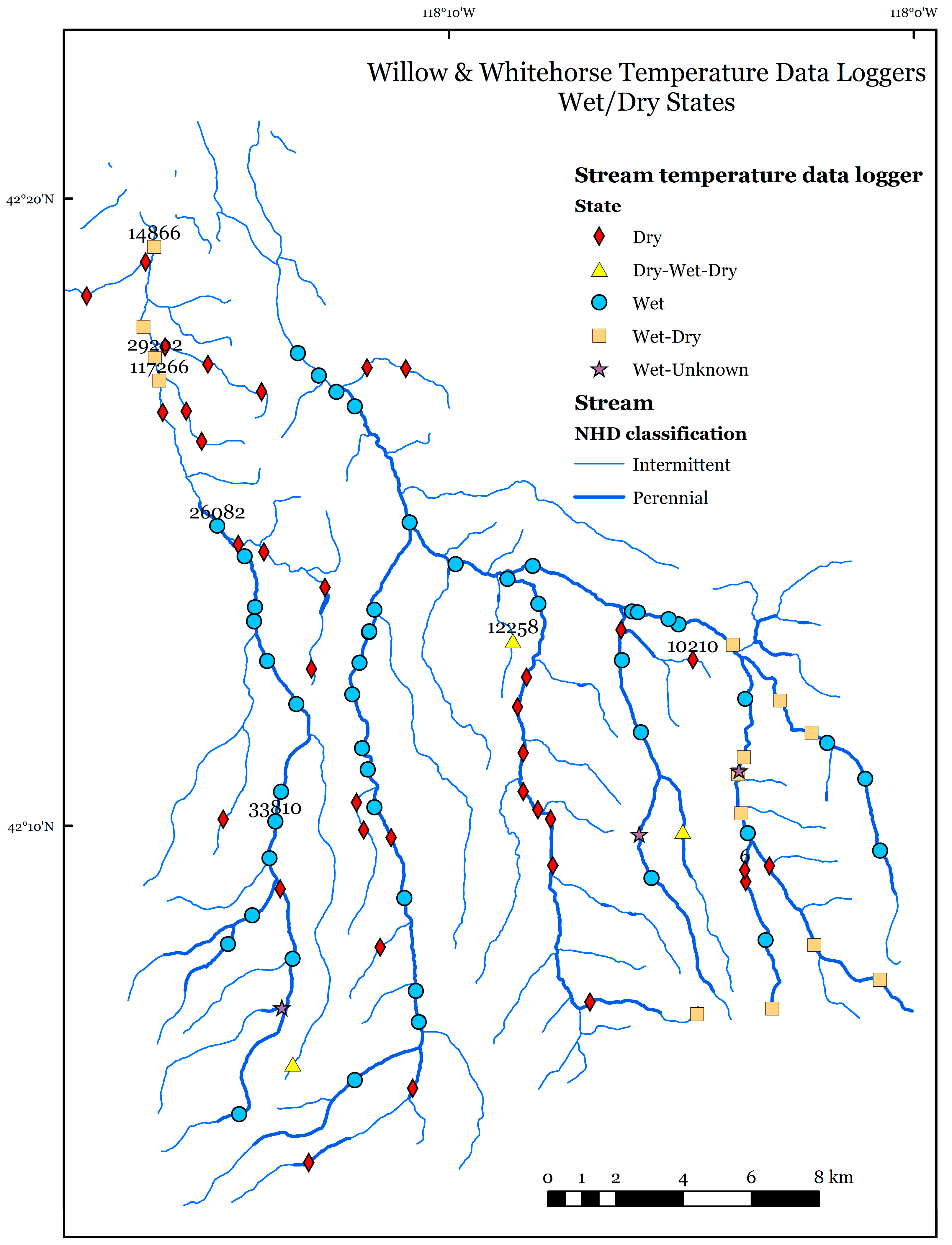
To examine spatial patterns of stream drying, we applied HMMs to 102 time series of daily SD of stream temperature at the WWC (Figure 5 and Figure 6). Our approach allowed us to identify both single and multiple states occurring among stream reaches during the period 1 April–27 August 2015. The majority of sites (80%) within WWC exhibited a single state with most of them (46%) having water over the entire time. There were also sites that showed one or more shifts among states (17%) with most of them shifting from wet to dry (14%). The cumulative number of sites that changed from wet to dry was useful to identify patterns of drying over time (Figure 5). There were two time periods that illustrated a rapid (5 June to 22 June 2015) versus a slow (23 June to 13 August 2015) pattern of drying (Figure 5c). The timing, duration and frequency of events (wet or dry) can also be extracted from this analysis as well as the spatial coherence among nearby sites. To provide a simple illustration, we mapped the presence of permanent wet or dry sites, as well as those that changed in state within the study time frame (1 April to 27 August 2015, Figure 6).
4. Discussion
Our findings demonstrate that Hidden Markov Models (HMMs) can effectively diagnose drying of stream channels based on patterns of variability in hourly recorded stream temperatures, without a need for data loggers specifically designed to detect drying [20]. Specifically, increases in the daily SD associated with the transition from water to air as streams dried produced a strong and predictable signal that was relatively easy to detect [10]. Though most methods to detect drying from temperature records are based on qualitative screens [9], application of Hidden Markov Models removes much, but not all, of the subjectivity that can be a limitation of such approaches.
Because we were interested in only two states in stream channels—wet or dry—we applied a two-state HMM to each sampled location. In cases where the true state was likely continuously dry or wet, the hidden Markov model produced unrealistically high frequency changes in states (e.g., seven or more within the time span we analyzed). Thus, as applied here, our choice of states and the decision to assign one or two states to any given site still involved an element of subjectivity, but less so than the level of subjectivity involved with existing methods of diagnosing drying [9]. Note here that we refer to drying at the point where our field data loggers were no longer in water. We deployed our instruments in the stream channel thalweg, therefore we are confident that if an instrument was no longer in water that the stream indeed dried at the sampled location, but we cannot extrapolate beyond that point (e.g., to intermittent reaches outside of the site or any conditions outside of the data logger itself).
As a general procedure to diagnose drying based on our findings, we recommend the following series of steps. To begin, we recommend initially plotting individual time series of stream temperature to visually identify potential anomalies. If available, information from nearby air temperature time series can be compared to stream temperatures to look for evidence of drying [9]. Following these steps, we recommend separating the time series into potential wet and dry seasons. In this study, we considered the dry season to be the time frame over which drying of streams was most likely (i.e., from 1 April into late summer). With this period of inference defined, an HMM can be applied to evaluate evidence for changes in state based on daily SD of temperature. If the HMM procedure results in an unexpectedly large number of changes among states (approximately seven in our study region) that do not relate to likely drivers of stream flow permanence (e.g., episodic patterns of water diversion, snowmelt, or precipitation), then there is likely only one true single state (wet or dry). To identify if the true single state represents wet or dry conditions, we recommend using air temperature time series from nearby sites as reference information. In our study region, for example, we reasoned that if maximum daily stream temperature was the same as maximum daily air temperature and both were above 30 °C, then the true state was likely dry. To further clarify whether a state represents the wet or dry condition of the site, we also used field notes describing the condition of data loggers during deployment and retrieval and available time series of air temperature. Finally, the assignment of states can be defined based on the table of probabilities (e.g., >0.5 for a given state) from the HMM output. Thus, we do not recommend diagnosing drying based on applications of HMMs alone, but rather as a complement to existing methods for screening temperature data [9,10].
Statistical issues aside, it is worth noting that the relatively arid systems we studied present a stark contrast between hydrologic (wet) and atmospheric (dry) conditions influencing heat fluxes, and thus the signal within the daily SD of temperatures. In very humid systems, or during times of the year when clouds, short photoperiods, snow cover, or other confounding factors could be in play, the thermal signature of water versus air may be less pronounced, and statistical pattern detection to diagnose drying may be less efficient. In such cases, the only alternative may be to deploy a more diverse data logger array [20] or alternative models for pattern detection in highly ephemeral systems [21]. It is also important to emphasize that we considered only a portion of the year (spring–summer) in this study. Studies of year-round variability in temperature [22] may encounter other changes in state, such as freezing in winter. Additional tests of the efficiency of HMMs for diagnosing drying under a broader range of conditions (continuous information on temperature with known patterns of drying) would be needed to more comprehensively evaluate where and when they are most likely to be useful. Given widespread and increasing amounts of stream temperature data collected from continuously recording temperature data loggers, information on flow permanence extracted from time series of temperatures using Hidden Markov Models offers potentially powerful new insights into patterns of flow permanence.
Although the question of flow permanence has drawn increasing attention in scientific and policy arenas [23], the fundamental problem of quantifying the status of flowing water in stream networks represents a long-standing challenge. Flow permanence in streams can be classified based on the processes that generate flows [24] and the corresponding timing, duration, and extent of flows at any given location [1]. Past stream flow permanence classifications have proven quite useful, but they may not be detailed enough to capture hydrologically and ecologically important dynamics in the timing, duration, frequency, and extent of flow events in stream networks [1] that are possible to extract from time series of temperature, as we have demonstrated here. Our application of HMMs across an entire stream network demonstrates the utility of this approach to describe patterns in the timing, duration, and frequency of flow permanence within a large watershed. Specifically, our findings show that most of the sites that were sampled within the stream network stay wet or dry during the entire season. In addition, some stream reaches synchronously shift from a wet to a dry state, but some sites shift sooner than others. In our study system, a detailed understanding of patterns of flow permanence was critical for identifying potential ecological responses of both aquatic and terrestrial species to seasonally and annually shifting patterns of water availability across the landscape [14]. Furthermore, our proposed method, in combination with modeling of flow duration curves (e.g., [25,26,27]), may be useful to understand shifts between wet and dry conditions or to determine minimum streamflow requirements in non-perennial (intermittent or ephemeral) streams.
In the context of possible drying of stream channels due to warming climates and increased probability of drought [14,28], understanding patterns of flow permanence in streams is paramount. Existing efforts to crowd-source stream temperature datasets across the northwest U.S., for example, have proven immensely valuable for predicting stream temperature across drainage networks and evaluating climate vulnerability for coldwater species [8]. However, these datasets are often biased towards perennial streams, as data from dry streams are typically removed [9]. The approach described herein highlights the value of such observations to contribute critical information on climate-sensitive patterns of flow permanence [1,5]. These, in turn, can be incorporated with information on thermal regimes from perennial streams to provide a more dynamic and comprehensive view of water quality and availability across broad spatial extents.
Acknowledgments
We would like to thank T. Allai, R. Flitcroft and S. L. Johnson for discussion and suggestions to improve this study. Fieldwork assistance was generously provided by C. Bailey, A. Berthold, J. Blake, B. Jones, M. McGuire, J. Pearson, B. Sempert, and A. Wong. Funding for this study was provided by the Vale office of the Bureau of Land Management, the U.S. Geological Survey Science Support Program, and the U.S. Geological Survey National Climate Change and Wildlife Science Center. Any use of trade, firm, or product names is for descriptive purposes only and does not imply endorsement by the U.S. Government. This manuscript is submitted for publication with the understanding that the United States Government is authorized to reproduce and distribute reprints for Governmental purposes. The data used in this publication can be accessed at https://doi.org/10.5066/F7BR8QFV and https://doi.org/10.5066/F7JQ0ZW2.
Author Contributions
I.A. designed and ran analysis, wrote and edited the paper; J.B.D. secured funding, designed study, wrote and edited the paper; M.P.H. designed study, collected data, and edited the paper; L.D.S. collected data, wrote and edited the paper; D.H.-W. collected data, manipulated data, and edited the paper.
Conflicts of Interest
The authors declare no conflict of interest.
References
- Jaeger, K.L.; Olden, J.D.; Pelland, N.A. Climate change poised to threaten hydrologic connectivity and endemic fishes in dryland streams. Proc. Natl. Acad. Sci. USA 2014, 38, 13894–13899. [Google Scholar] [CrossRef] [PubMed]
- Datry, T.; Arscott, D.B.; Sabater, S. Recent perspectives on temporary river ecology. Aquat. Sci. 2011, 73, 453–457. [Google Scholar] [CrossRef]
- Morisawa, M.E. Accuracy of determination of stream lengths from topographic maps. Eos Trans. AGU 1957, 38, 86–88. [Google Scholar] [CrossRef]
- Fritz, K.M.; Hagenbuch, E.; D’Amico, E.; Reif, M.; Wigington, P.J., Jr.; Leibowitz, S.G.; Comeleo, R.L.; Ebersole, J.L.; Nadeau, T. Comparing the Extent and Permanence of Headwater Streams from Two Field Surveys to Values from Hydrographic Databases and Maps. J. Am. Water Resour. Assoc. 2013, 49, 867–882. [Google Scholar] [CrossRef]
- Sando, R.; Blasch, K.W. Predicting alpine headwater stream intermittency: A case study in the northern Rocky Mountains. Ecohydrol. Hydrobiol. 2015, 15, 68–80. [Google Scholar] [CrossRef]
- Constantz, J.; Stonestrom, D.; Stewart, A.E.; Niswonger, R.; Smith, T.R. Analysis of streambed temperatures in ephemeral channels to determine streamflow frequency and duration. Water Resour. Res. 2001, 37, 317–328. [Google Scholar] [CrossRef]
- Bhamjee, R.; Lindsay, J.B. Ephemeral stream sensor design using state loggers. Hydrol. Earth Syst. Sci. 2011, 15, 1009–1021. [Google Scholar] [CrossRef] [Green Version]
- Isaak, D.J.; Wenger, S.J.; Peterson, E.E.; Ver Hoef, J.M.; Hostetler, S.W.; Luce, C.H.; Dunham, J.B.; Kershner, J.L.; Roper, B.B.; Nagel, D.E.; et al. NorWeST Modeled Summer Stream Temperature Scenarios for the Western U.S. Fort Collins, CO. For. Serv. Res. Data Arch. 2016. [Google Scholar] [CrossRef]
- Sowder, C.; Steel, E.A. A note on the collection and cleaning of water temperature data. Water 2012, 4, 597–606. [Google Scholar] [CrossRef]
- Blasch, K.W.; Ferré, T.; Hoffman, J.P. A statistical technique for interpreting streamflow timing using streambed sediment thermographs. Vadose Zone J. 2004, 3, 936–946. [Google Scholar] [CrossRef]
- Dunham, J.B.; Chandler, G.L.; Rieman, B.E.; Martin, D. Measuring Stream Temperature with Digital Data Loggers: A User’s Guide; Rocky Mountain Research Center General Technical Report RMRS-GTR-150WWW; U.S. Dep. Agric., Forest Service: Fort Collins, CO, USA, 2005. [CrossRef]
- Zucchini, W.; MacDonald, I. Hidden Markov Models for Time Series: An Introduction Using R, 1st ed.; CRC Press: Boca Raton, FL, USA, 2009; ISBN 978-1-58488-573-3. [Google Scholar]
- Blasch, K.W.; Ferré, T.; Christensen, A.H.; Hoffman, J.P. New field method to determine streamflow timing using electrical resistance sensors. Vadose Zone J. 2002, 1, 289–299. [Google Scholar] [CrossRef]
- Schultz, L.D.; Heck, M.P.; Hockman-Wert, D.; Allai, T.; Wenger, S.; Cook, N.A.; Dunham, J.B. Spatial and temporal variability in the effects of wildfire and drought on thermal habitat for a desert trout. J. Arid Environ. 2017, 145, 60–68. [Google Scholar] [CrossRef]
- Heck, M.P.; Schultz, L.D.; Hockman-Wert, D.; Dinger, E.; Dunham, J.B. Monitoring stream temperatures: A guide for non-specialists. 2017; manuscript in preparation. [Google Scholar]
- Chapin, T.P.; Todd, A.S.; Zeigler, M.P. Robust, low-cost data loggers for stream temperature, flow intermittency, and relative conductivity monitoring. Water Resour. Res. 2014, 50, 6542–6548. [Google Scholar] [CrossRef]
- Visser, I. Seven things to remember about hidden Markov models: A tutorial on Markovian models for time series. J. Math. Psychol. 2011, 55, 403–415. [Google Scholar] [CrossRef]
- Visser, I.; Speekenbrink, M. depmixS4: An R Package for Hidden Markov Models. J. Stat. Softw. 2010, 36, 1–21. [Google Scholar] [CrossRef]
- R Development Core Team. R: A Language and Environment for Statistical Computing; R Foundation for Statistical Computing: Vienna, Austria, 2011; ISBN 3-900051-07-0. [Google Scholar]
- Bhamjee, R.; Lindsay, J.B.; Cockburn, J. Monitoring ephemeral headwater streams: A paired sensor approach. Hydrol. Process. 2016, 30, 888–898. [Google Scholar] [CrossRef]
- Gungle, B. Timing and Duration of Flow in Ephemeral Streams of the Sierra Vista Subwatershed of the Upper San Pedro River Basin, Cochise County, Southeastern Arizona; Scientific Investigations Report 2005–5190, Govt. Doc. Number I 19.42/4-4:2005-5190; United States Geological Survey: Reston, VA, USA, 2006.
- Arismendi, I.; Johnson, S.L.; Dunham, J.B. Technical Note: Higher-order statistical moments and a procedure that detects potentially anomalous years as two alternative methods describing alterations in continuous environmental data. Hydrol. Earth Syst. Sci. 2015, 11, 1169–1180. [Google Scholar] [CrossRef]
- Acuña, V.; Datry, T.; Marshall, J.; Barcelo, D.; Dahm, C.N.; Ginebreda, A.; McGregor, G.; Sabater, S.; Tockner, K.; Palmer, M.A. Why should we care about temporary waterways? Science 2014, 343, 1080–1081. [Google Scholar] [CrossRef] [PubMed]
- Meinzer, O.E. Plants as Indicators of Groundwater; Water Supply Paper 577; United States Geological Survey: Washington, DC, USA, 1927. Available online: https://pubs.usgs.gov/wsp/0577/report.pdf (accessed on 2 December 2017).
- Botter, G.; Zanardo, S.; Porporato, A.; Rodriguez-Iturbe, I.; Rinaldo, A. Ecohydrological model of flow duration curves and annual minima. Water Resour. Res. 2008, 44, W08418. [Google Scholar] [CrossRef]
- Iacobellis, V. Probabilistic model for the estimation of T year flow duration curves. Water Resour. Res. 2008, 44, W02413. [Google Scholar] [CrossRef]
- Pumo, D.; Viola, F.; La Loggia, G.; Noto, L.V. Annual flow duration curves assessment in ephemeral small basins. J. Hydrol. 2014, 519, 258–270. [Google Scholar] [CrossRef]
- Diffenbaugh, N.S.; Swain, D.L.; Touma, D. Anthropogenic warming has increased drought risk in California. Proc. Natl. Acad. Sci. USA 2015, 112, 3931–3936. [Google Scholar] [CrossRef] [PubMed]
Figure 1.
Map of watersheds within the northwest hydrographic Great Basin in southeast Oregon (Willow and Whitehorse Creek watershed—WWC, top) and north-central Nevada (Willow and Rock Creek watershed—WRC, bottom) from which data were collected and applied in this study. Within WWC, blue circles indicate locations where stream temperature was monitored, and yellow diamonds indicate locations where both temperature and electrical resistance were monitored. In WRC, both air and stream channel temperatures were monitored.

Figure 2.
Conceptual model that illustrates the use of daily standard deviation (SD) of stream temperature as the input metric for Hidden Markov Models (HMMs) for signal detection. The upper figure illustrates several metrics of stream temperature and the lower figure shows the output of using daily SD of stream temperature as a signal to separate wet and dry states. The timing (t1, start, t1, end) and duration (d1,1) of the events (event 1 is defined as t1, d1) can provide useful information to identify spatiotemporal patterns of stream drying over time.

Figure 3.
Illustrative examples of the use of time series of daily standard deviation of stream temperature as inputs for Hidden Markov Models (HMMs) at eight stream reaches from the Willow and Rock Creek watershed (WRC) between 1 April and 27 July 2016. Time series of paired air temperature loggers deployed at the same sites can be used as confirmatory information about states. Similar diel fluctuations between stream and air temperature indicate dry conditions whereas the opposite represents wet conditions. The left panel illustrates patterns of stream drying including wet–dry conditions over time. The right panel illustrates purely wet conditions of stream reaches even though HMMs identify multiple shifts among states. Under such circumstances, contrasting hourly values of stream versus air temperature can be used as confirmatory information of the type of single state.

Figure 4.
Illustrative examples of the use of time series of daily standard deviation of stream temperature as inputs for Hidden Markov Models (HMMs) at eight stream reaches from the Willow and Whitehorse Creek watershed (WWC) between 1 April and 27 August 2015. Time series of paired modified electrical resistance loggers deployed at the same sites can be used as confirmatory information about states. Negative values of electrical resistance indicate dry conditions whereas positive values represent wet conditions. The left panel illustrates patterns of stream drying including dry–wet–dry (site12258) and wet–dry (site117266, site29202, and site14866). The right panel illustrates purely wet (site33810, site26082) and purely dry (site00006, site10210) conditions of stream reaches even though HMMs identify multiple shifts among states. Under such circumstances, daily mean and hourly values of stream temperature can be used as confirmatory information of the type of single state.

Figure 5.
Spatiotemporal patterns of stream drying using time series of daily standard deviation of stream temperature as inputs for Hidden Markov Models (HMM) at 102 stream reaches from the Willow and Whitehorse Creek watershed (WWC) between 1 April and 27 August 2015. (a) Timing of shift between states among stream reaches. (b) Proportion of stream reaches having single and multiple states over time (unknown = state that accounts for a decrease in daily SD. This is due to data loggers that were buried in sediment or possibly due to the influence of groundwater). (c) Cumulative distribution of sites that shifted from wet to dry states.
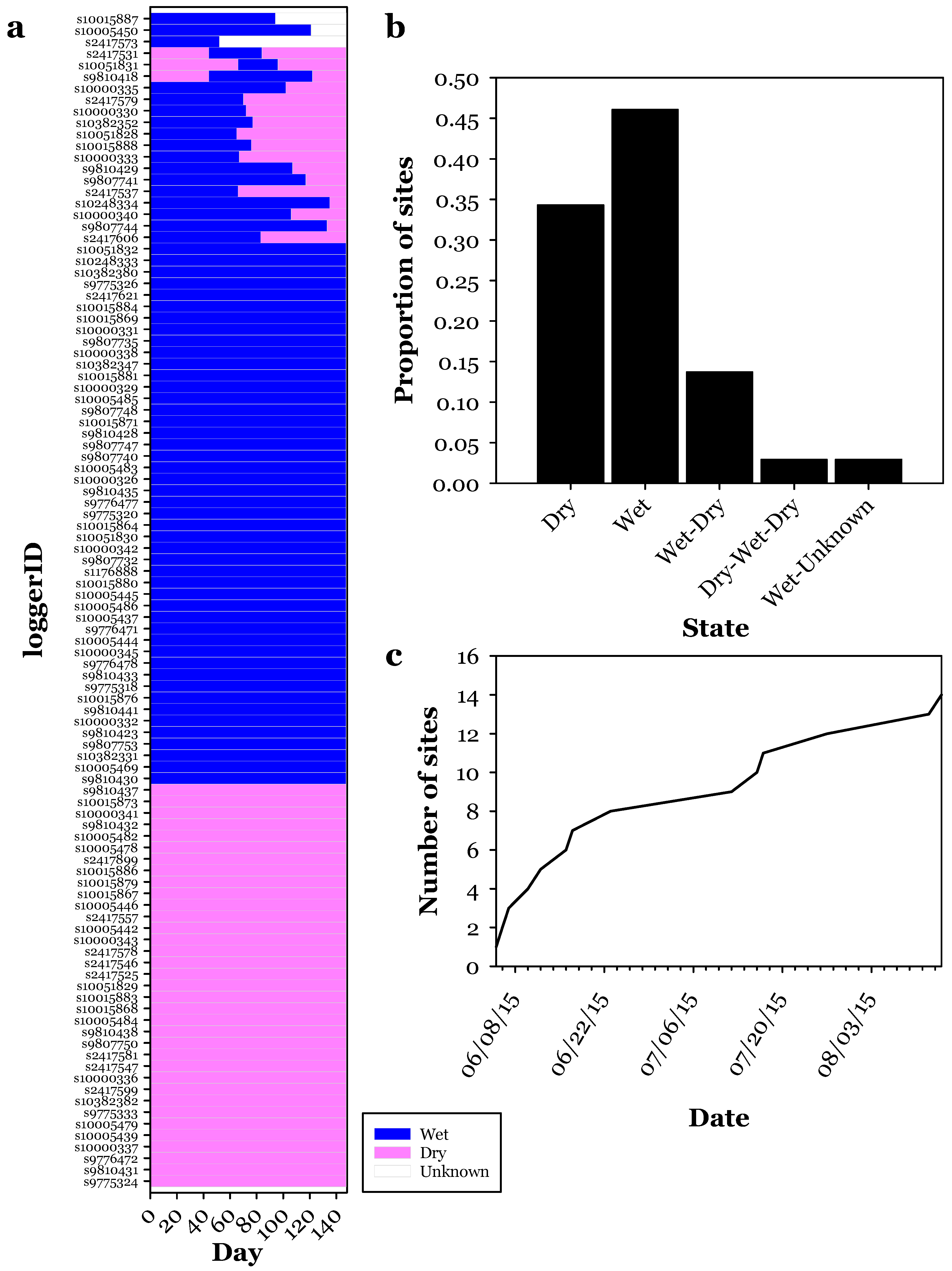
Figure 6.
Map of Willow and Whitehorse Creek watershed, OR, with location of points within the network indicating changes in the states of streams (Figure 5). Numbered sites correspond with those shown above (Figure 4). Streams shown are from the 1:100,000 scale National Hydrography Dataset (available at https://nhd.usgs.gov/).

© 2017 by the authors. Licensee MDPI, Basel, Switzerland. This article is an open access article distributed under the terms and conditions of the Creative Commons Attribution (CC BY) license (http://creativecommons.org/licenses/by/4.0/).
Share and Cite
MDPI and ACS Style
Arismendi, I.; Dunham, J.B.; Heck, M.P.; Schultz, L.D.; Hockman-Wert, D. A Statistical Method to Predict Flow Permanence in Dryland Streams from Time Series of Stream Temperature. Water 2017, 9, 946. https://doi.org/10.3390/w9120946
AMA Style
Arismendi I, Dunham JB, Heck MP, Schultz LD, Hockman-Wert D. A Statistical Method to Predict Flow Permanence in Dryland Streams from Time Series of Stream Temperature. Water. 2017; 9(12):946. https://doi.org/10.3390/w9120946
Chicago/Turabian StyleArismendi, Ivan, Jason B. Dunham, Michael P. Heck, Luke D. Schultz, and David Hockman-Wert. 2017. "A Statistical Method to Predict Flow Permanence in Dryland Streams from Time Series of Stream Temperature" Water 9, no. 12: 946. https://doi.org/10.3390/w9120946
Note that from the first issue of 2016, this journal uses article numbers instead of page numbers. See further details here.