Measurement and Simulation of Soil Water Contents in an Experimental Field in Delta Plain


1
State Key Laboratory of Hydrology-Water Resources and Hydraulic Engineering, Hohai University, Nanjing 210098, China
2
College of Hydrology and Water Resources, Hohai University, Nanjing 210098, China
*
Author to whom correspondence should be addressed.
Water 2017, 9(12), 947; https://doi.org/10.3390/w9120947
Submission received: 8 October 2017
/
Revised: 27 November 2017
/
Accepted: 2 December 2017
/
Published: 6 December 2017
(This article belongs to the Special Issue Soil Water Conservation: Dynamics and Impact)
Abstract
:Variation in soil water content in the delta plain has its own particularity and is significant for agricultural improvement, the utilization of water resources and flood risk mitigation. In this study, experimental data collected from a plot of farmland located in the Taihu Basin were used to investigate the temporal and vertical variation of soil water content, as well as the effects of individual rainfall on soil water and shallow groundwater and their interaction. The results showed that the variation of soil water content is dependent on the comprehensive influence of soil hydraulic properties, meteorological factors and shallow groundwater and the correlation to the groundwater table is the strongest due to the significant capillary action in the delta plain. A saturated-unsaturated three-dimensional soil water numerical model was developed for the study area in response to rainfall and evapotranspiration. Scenario simulations were performed with different soil depths for soil water content and the error source was analyzed to improve the model. The average RMSE, RE and R2 values of the soil water content at the five depths between the measured and simulated results were 0.0192 cm3·cm−3, 2.09% and 0.8119, respectively. The results indicated that the developed model could estimate vertical soil water content and its dynamics over time at the study site at an acceptable level. Moreover, further research and application to other sites in delta plains are necessary to verify and improve the model.
1. Introduction
Most delta plains are lowlands, which are often densely populated and form centers of agricultural production, economic activity and transportation [1] such as the Taihu Basin in the Yangtze River Delta, East China, approximately 30% of which are lowland polders [2]. However, these areas are characterized by low elevation, flat topography, a shallow groundwater table, extensive river networks and uncertain catchment boundaries [3,4,5]. Therefore, delta plains require more attention to keep out natural hazards given their vulnerability to flooding, climatic variation and water quality deterioration. To avoid and mitigate the effects of natural and artificial disasters, exploring and simulating the specific hydrologic processes of delta plains are quite important for regional risk assessment and water resource engineering design.
Soil water content is a key state variable in the terrestrial system as it interacts with various system components [6,7] and is of great importance in many investigations and applications pertaining to agriculture, hydraulic engineering, hydrology, meteorology and soil mechanics [8,9,10]. Climatic conditions [11], vegetation types [12,13,14], topography [15], soil properties [16,17], antecedent soil water content [18] and hysteresis [19,20] determine the spatio-temporal variability of soil water content [21], which in turn affects the exchange of energy and water in the unsaturated zone of the hydrological system [22]. These exchange processes are characterized by high nonlinearity and complex feedback mechanisms [6]. Consequently, different measurement technologies (e.g., sensor technologies and distributed sensor networks [23,24,25]) and simulation models have been used to study the importance of soil water content for describing and understanding vadose zone processes [26], climate and atmospheric processes [27], soil moisture estimation [28] and so on.
There are two main approaches for soil water study and prediction: field observation-based and modeling-based methods. As one of the dielectric-based techniques to determine soil water content at the local scale, the well-known time domain reflectometry (TDR) was introduced by Topp et al. [29] and has developed into a standard method to measure soil water content. It provides the apparent relative dielectric permittivity of soil determined by monitoring the travel time of a fast-rise-step voltage pulse along a transmission line connected to a suitable probe placed in the soil at the required measuring depth [8]. Nevertheless, observations of shallow groundwater and meteorology (e.g., temperature, rainfall and evaporation) should also be considered and applied to models when simulating soil water content. Two of the most widespread soil water models are the Richards equation-based models and the Bucket model. HYDRUS [30,31], which numerically solves the Richards equation for saturated–unsaturated water flow and convection–dispersion type equations for heat and solute transport, has been widely used to analyze the multi-layer soil water flow for preferential flow [32,33,34,35], transport domains for both laboratory [36,37] and field-scale applications [38,39]. However, it is not recommended to use HYDRUS for very large 3D domains such as entire catchments [40]. For certain types of applications, a successful synopsis of both monitoring and modeling issues was presented by Morbidelli et al. [41] that referred to the experimental field campaigns carried out to measure the soil water content with the TDR method in the vertical soil profiles of five different plots. However, it was not designed for delta plains with shallow groundwater. Some models coupling surface water to groundwater can also be used for soil water dynamics analysis or simulation. The SWATMOD model [42] is the coupling of the SWAT model and the MODFLOW model but tends to simulate soil percolation which skips unsaturated soil water. The MODBRNCH model [43] develops a pattern to connect the MODFLOW model and the BRNCH model where Saint-Venant equations need to be solved with much shorter steps than in the former. There are other models, like the HSPF-MODFLOW model, GSFLOW model, MODFLOW-DAFLOW model, IFM Mike model, IGSM model [44], etc., where most of these models are the direct coupling of two mature models referring to saturated and understanding the soil water, respectively, which saves much work but also has their own shortages and limitations. Furthermore, the two sub models are in an unconsolidated couple by infiltration but with independent processes and calculations. Comparatively, the Mike-SHE model [45] developed by the Danish Institute of Water Conservancy is complete with different functions but it is a model based on the actual physical process which needs a large amount of hydrologic data, topographic map and parameters. Therefore, a simplified specific model is required for conducting research in a particular location to greatly improve work efficiency, especially as the basis for an upscaling model in further work. Meanwhile, field observation is an important and pervasive way to support analysis and verification.
In this study, an experimental field was introduced in detail and measured data were analyzed in different ways. A three-dimensional numerical model was built up, calibrated and validated for the soil water flow at the study site based on the Richards equation. The basic research into soil water and addressing this as a backbone for specific model development will help us understand various hydrological processes, provide reference to improving agricultural planning and more accurate hydrological prediction. Three objectives of this study are proposed: (1) Construct a special experimental field with necessary instruments in the Yangtze River Delta to make future experiments more targeted, operable and flexible; (2) Explore the temporal and vertical variations of soil water content, the effects of individual rainfall on soil water and shallow groundwater and their interaction; (3) Seek a simplified special model for soil water estimation in the delta plain. In this paper, the field experiments and the numerical methods are provided in Section 2. The data analyses and modeling results for soil water are presented in Section 3. Several significant points are discussed in Section 4. Conclusions are made in Section 4.
2. Materials and Methods
2.1. Site, Soil Sampling and Instrumentation
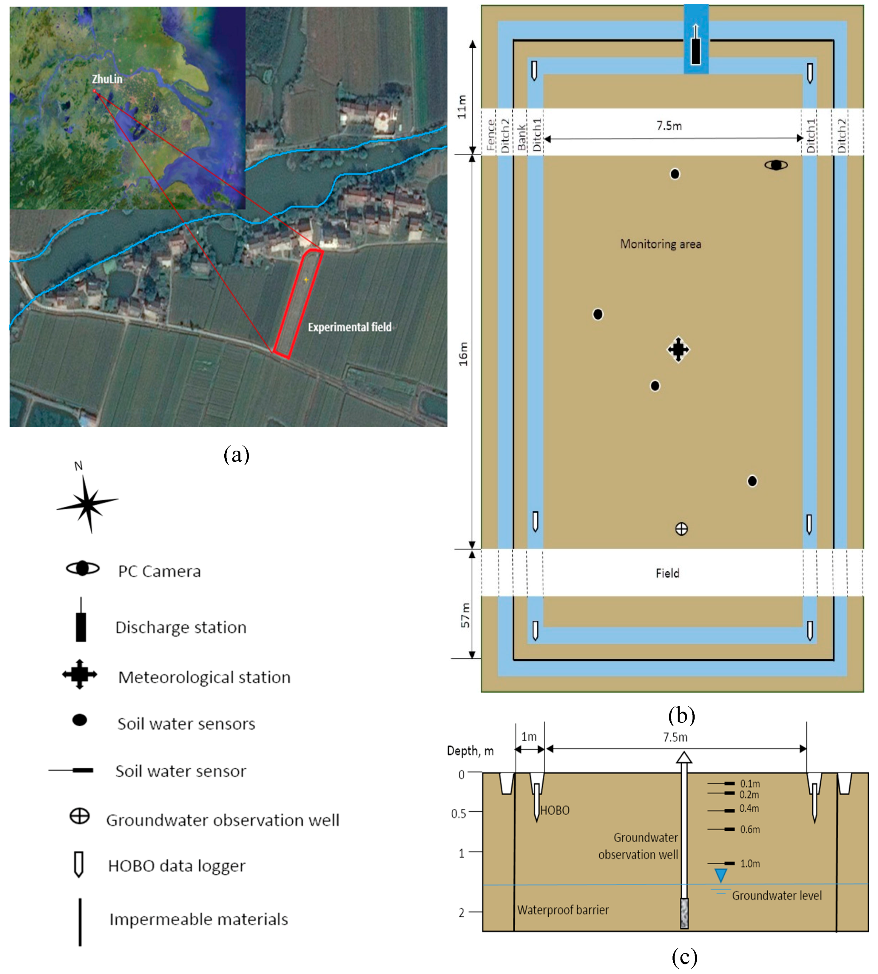
The study site for the hydrological observation and field experiment is located in ZhuLin, Changzhou City in China (Figure 1a). It is part of the Taihu Basin in the Yangtze River Delta and is characterized by flat terrain and a river network. The region has a subtropical monsoon climate with 900–1100 mm annual rainfall and 1000–1500 mm annual evaporation. The soil consists of a 30 m deposit of Quaternary. The upper 0.55–0.6 m soil layer is plain fill with high clay and the lower 0.7–0.9 m consists of silty clay. From 1.9 to 3.2 m below the ground surface, the third layer is mainly composed of silt and silty sand. The phreatic water table level is located at approximately 1 m in depth. The saturated hydraulic conductivity (K) is around 3 × 10⁻⁴ m/s according to testing results.
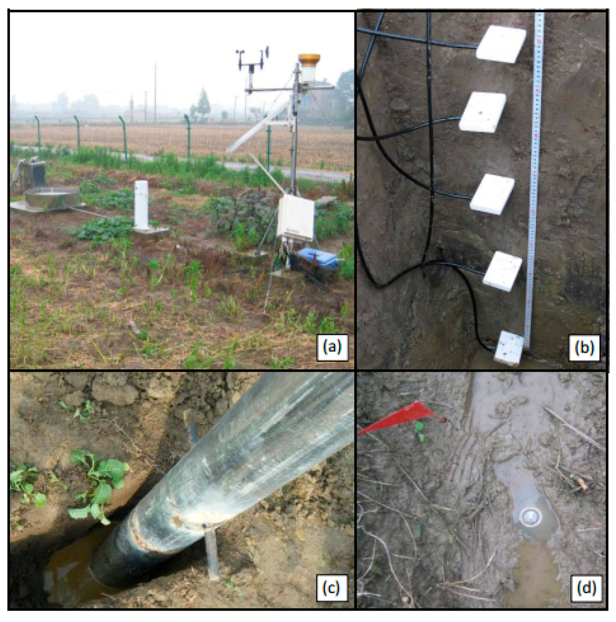
The experimental field is isolated from the surrounding surface water with a waterproof barrier. Two drainage ditches inside and outside the impermeable materials are linked at the outlet leading to a river. Figure 1b shows the layout of the field, which has an area of 798 m2 with a length of 84 m and width of 9.5 m. Measuring instruments installed there included a video camera, a discharge meter next to a V-notch weir, a meteorological station, four soil water profiles, a groundwater observation well and some HOBO data loggers (Figure 2). Meteorological factors such as rainfall, evaporation, temperature, wind speed and direction were measured by the meteorological station. The measurements of soil water content at different depths (10, 20, 40, 60 and 100 cm) of soil profile were performed by the soil water sensors (TDR100, Campbell Scientific) and were recorded at intervals of 10 min in terms of volumetric water content obtained from the TDR signal through the universal calibration curve of Topp et al. [29]. The phreatic water table was recorded continuously with a time step of 5 min by the groundwater observation well. The HOBO data loggers recorded the water table and temperature in the ditch with a time step of 5 min. Detailed information on the vertical layout of the field is shown in Figure 1c.
Soil samples were collected using a corner with a 100 cm3 volume sample ring at 0.10, 0.20, 0.40, 0.60 and 1.00 m depths near the sensor probe below the ground surface in the experimental field. First, the oven-drying method was used to verify the accuracy of the soil water content measured by the sensor. The results indicated that the value measured by the sensor was systematically higher than by the oven-drying method. The range of calibrated soil water content was further determined by the membrane pressure gauge method. The soil water content at a pressure of 0 kPa and 30 kPa was determined as the saturated value (maximum) and the field capacity (minimum), respectively. The rest of the soil water content data were calibrated in proportion. Pan evaporation measured by the evaporation gauge (255-100 Novalynx Analog Output Evaporation Gauge, Campbell Scientific, Inc., Logan, UT, USA) was used to calculate potential evapotranspiration. The physical properties and grain composition of soil samples at 10, 20, 40, 60 and 100 cm depths in the north, center and south of the experimental field were measured by certified professionals. Some of the results are shown in Table 1, which can presumably reflect the spatial heterogeneity of soil.
2.2. Mathematic Model and Parameters
2.2.1. Equations of Saturated-Unsaturated Soil Water Flow
Water moves from where the soil water potential is higher to where it is lower. The soil water potential in the unsaturated zone is constructed of gravitational potential and matric potential, while the saturated zone is composed of gravitational potential and pressure potential. Gravitational potential is expressed as the pressure head of vertical position, z; pressure potential shows as the positive pressure head, h; and matric potential is represented as the negative pressure head, h, based on the assumption of a 0 air pressure. Soil water potential, ψ, is expressed as pressure head, h.
The Darcy Buckingham equation [46] is substituted into the continuity equation based on the principle of mass conservation and the storage term is modified to construct saturated-unsaturated flow conditions, then the 3D Richards equation in partial differential form expressed by the pressure head h is as follows:
where Kx(h), Ky(h) and Kz(h) are the hydraulic conductivities in the x, y and z directions, respectively; h is the pressure head (L); and W is a volumetric source or sink term (L3·L−3·T−1) including rainfall infiltration, evapotranspiration and so on. C(h) is the specific moisture capacity (L−1); Sf is the saturation ratio (=θ/η); θ is the moisture content; η is the porosity; and us is the specific storage (L−1). Equation (1) involving the saturated zone is called the modified Richards equation [47].
Hydraulic conductivity can be calculated from this empirical equation by the Van Genuchten [48] parametric functions:
where Ks is the saturated hydraulic conductivity; h is the pressure head; α and n are fitting parameters in the soil water retention curve; and m = 1 − 1/n, n > 1.
Paniconi et al. [49] modified van Genuchten and Nielsen’s [48] closed-form equation for hydraulic conductivity using the moisture retention curve. Thus, the specific moisture capacity C(h) can be calculated by:
where θr is the residual water content; θs is the saturated soil water content; β = (|h/hs|)n; hs is the air entry pressure head (L); n is a fitting parameter in the soil water retention curve; m = 1 − 1/n; and h0 is a parameter solved on the basis of a given value of C(h) = us.
2.2.2. Rainfall Infiltration
Rainfall and evapotranspiration are treated as the volumetric source or sink term (W) in the modified 3D Richards equation. The rainfall is going down and up is taken to be the positive direction for the z-axis, so the infiltration rate of the land surface is defined as Iz2. The value of Iz2 is dependent on the magnitude relationship between rainfall intensity and infiltration capacity, which is equal to the smaller one. The volumetric source from rainfall can be calculated as follows:
where is the area of the grid cell.
2.2.3. Potential Evapotranspiration
Evapotranspiration in this model is treated as a combination of transpiration and evaporation. Potential evapotranspiration (PET) can be calculated using two different options. The first option is the pan evaporation technique, which requires daily measured pan evaporation values and pan coefficients. In this method, PET is calculated as:
where Cpan is the pan coefficient, which is generally equal to approximately 0.7; and Epan is the measured pan evaporation [50]. Actual evaporation (Ea) is assumed to be equal to PET in the moist areas empirically and applied to the land surface as a negative flux boundary condition.
2.3. Boundary Conditions
In this model, variable boundary conditions are used to describe rainfall (infiltration) and evapotranspiration processes. The rainfall reaching the land surface is treated as a specified flux boundary condition. If the total head on the land surface is greater than the maximum ponding depth, this means that the infiltration capacity has been reached and the boundary condition is changed to a specified head boundary condition. Similarly, the evapotranspiration is applied to an outward flux boundary at the surface (i.e., a Neumann boundary) until water arrives at the top surface of the soil. Then, if the soil water content is reduced to a specified minimum water content, the boundary conditions are set to a prescribed minimum pressure (i.e., a Drichlet boundary), which infrequently occurs considering the climate characteristics in this region. The maximum potential evapotranspiration is first calculated [22].
The boundary condition at the bottom was specified as a free drainage condition and the water flux through the bottom was considered as an approximation of groundwater recharge due to the soil water contents in the deep (more than 100 cm) being relatively steady. The soil water pressure and pressure head at the water table at the beginning of each simulation period were used to characterize the initial condition. The soil water pressures can be calculated by the van Genuchten model with the soil water content measured by the soil water content sensor. The measured value of the pressure head at the water table is zero.
2.4. Model Calibration
Relative error (RE), root-mean squared error (RMSE) and the coefficient of correlation (R2) between the simulated and observed soil water content were calculated to evaluate the accuracy of the model [51,52]:
where Oi is the observed; Si the simulated soil water content and n is the sample size. The match between the model prediction and observation increased as the relative error and root-mean squared error decreased.
3. Results and Discussion
3.1. Data Set Analysis
Figure 3 presents several meteorological elements and volumetric soil water content observed at the experimental field during 2014. Rainfall was mostly concentrated between April and September, with the maximum appearing in July reaching about 100 mm a day. The evaporation had roughly same tendency as the daily mean temperature. The trend of soil water content of the topsoil at the depth of 10 cm resembled that of the daily mean temperature and rainfall [53]. It changed less than the daily mean temperature but had large fluctuations (the greatest variation was about 37%) with rainfall. The soil water content at five depths had similar varying tendency, while the fluctuation range became smaller and values gradually increased from a depth of 10 cm to 100 cm. Higher values of soil water content appeared between the depths of 60 cm and 100 cm, ranging from 0.44–0.563.
3.1.1. Effect of Rainfall on the Soil Water Content
To investigate the impact of rainfall on soil water content at different depths, a representative rainfall event was selected to record the soil water content in a soil profile before, during and after it with a time step of one hour (Figure 4a). Before the rain, the soil water content first increases, then decreases with increasing soil depth, where the maximum was 0.458 at a depth of 60 cm. This difference may be caused by the combined effect of evapotranspiration, the supply of shallow groundwater and disparities in soil property at different depths. The increasing soil depth produced a mild drag on the increase of soil water content with the rainfall, which may be due to different field capacities. The soil water content of the topsoil increased greatly at a depth of less than 40 cm and the maximum increment at 0.2 appeared at a 10 cm depth. The soil water content at the depths of 60 cm and 100 cm were similarly always the maximum, while producing relative minimum increments of 0.03 with the rainfall. The soil water content at the depths of 10 cm and 2 0 cm stopped increasing and at 20 cm and 40 cm depths tended to be the same after the rainfall process.
In comparison, the decrease of soil water content is mainly caused by evapotranspiration without human activity. The pan evaporation measured in this experimental field was used to calculate potential evapotranspiration in the model. A 12-day evaporation period is shown in Figure 4b, which indicated that the soil water content decreased mostly at a depth of less than 20 cm, particularly in the topsoil at a 10 cm depth with the evaporation. The differences between Figure 4a,b suggested that the soil water content was more sensitive to rainfall than evapotranspiration and that the effects of rainfall could reach deeper soil layers. Therefore, soil water contents above the 20 cm depth are essentially controlled by rainfall and evapotranspiration [20] and those below the 40 cm depth are mainly controlled by rainfall and shallow groundwater in this field.
3.1.2. Combined Effects of Rainfall and Water Table Depth on Soil Water Content
The experimental field where the study was conducted is a typical site in the Taihu Basin with a river network. Figure 5b–f show the variations in shallow groundwater table (depth: 0.237–1.491 m) and soil water contents (θ: 0.266–0.563) at the depths of 10, 20, 40, 60 and 100 cm during different rainfalls. The annual dynamic changes in Figure 5a presents a positive correlation between the water table depth and soil water content between depths from 10 cm and 60 cm. The soil water content increases with increasing soil depth when the shallow groundwater table falls and is at a relatively low level with no rainfall. However, when the water table starts to rise, the distribution rule begins to be broken due to the rainfall. The soil water content at a depth less than 10 cm can usually go beyond that at depths between 20 cm and 40 cm under rainfall, while the soil water content at depths of 60 cm and 100 cm (θ: 0.44–0.563) are always much greater than the others (θ: 0.266–0.492). Soil water content at a depth of 100 cm is relatively stable with values around 0.513 and its slight increase appears earlier than the rising of the water table. This indicates that the soil water and groundwater are mainly supplied by rainfall and the soil water content at the depths of more than 100 cm can obtain enough recharge from the groundwater [54] by capillary pressure to remain fairly constant when there is little or no rain. However, the soil water content at depths less than 60 cm can increase considerably and quickly with rainfall and decrease gradually with evaporation as it is too far relatively to receive enough groundwater recharge.
Furthermore, the soil water content at a depth of 100 cm decreases when the water table falls to where it is still above the depth of 1 m. This may be due to the falling water table decreasing the pressure on the residual gas in the soil pore, so that the volume of gas becomes relatively greater and the soil water content decreases. Similarly, the special stage where soil water content at a depth of 60 cm exceeds that at a depth of 100 cm occurs when the shallow groundwater table is above a depth of 60 cm for a fairly long period of time. This may be caused by the difference of soil properties [55] at the two depths and the rising water table above a depth of 60 cm increases the pressure on the gas in the soil pore at a depth of 60 cm, which makes the volume of gas relatively smaller and the soil water content greater.
The rainfall conditions and details of shallow groundwater table for Figure 5b–f are given in Table 2. When the rainfall was as small as 9.3 mm (Figure 5b), only the soil water content at depths of 10 cm and 20 cm increased by 0.051 (16.5%) and 0.017 (5.1%), respectively. Instead of rising after the rain, the shallow groundwater table fell by 0.079 m (8.3%). This was because the long period of rainfall before had allowed the water table to rise significantly and then began to fall with evaporation, despite this small rain. At the same time, the soil water content of the deep layers remained relatively stable for capillary rise [56,57]. When the rainfall increased to 17.5 mm (Figure 5c) and 30.8 mm (Figure 5d), the water table rose by 0.065 m (5.2%) and 0.360 m (31.0%), respectively. This difference was caused by a relatively high-intensity rainfall and a low initial water table for the latter. During these two rainfall events, the soil water content at depths of 10, 20 and 40 cm all increased and the increment decreased with the increase of depth, which ranged from 0.091–0.019 (27.7–5.0%) for the former and 0.129–0.025 (46.2–7.1%) for the latter. The difference was that, in the former case, the value of the soil water content at a depth of 60 cm approached that of a depth of 100 cm and remained increasing, while in the latter case, the soil water content at a depth of 100 cm was 0.06 greater and increased much more than that at a depth of 60 cm. This indicates that only when the rainfall intensity is high enough can the soil water content at depths of more than 100 cm increase remarkably or quickly. Additionally, the soil water content at a depth of 60 cm in May was generally greater than that in March, which suggested that evaporation was less able to influence the deep soil layer with the onset of the rainy season and intermittent rains could make the soil water content at depths less than 60 cm change with the seasons [20,53], forming an annual cycle similar to a cosine curve (Figure 5a). However, soil water content and shallow groundwater table tend to be steady values when the rainfall was more intense or heavier. Figure 5e,f show that under rainfalls of 72.3 mm and 138.6 mm, respectively, the rainfall intensity of the former was nearly three times higher than the latter. The soil water content at a depth of 10 cm increased 0.118 more under conditions of higher intensity than a larger amount of rainfall. Although the soil water content at the other depths in the former case all increased normally, only that at a depth of 20 cm increased by 2.7% in the case of the latter. Furthermore, the water table rose by only 0.056 m with the largest amount of rainfall in this study, which was only one tenth that of the former. The differences indicate that the shallow groundwater table is greatly controlled by rainfall and evaporation and the initial depth of the water table decides the sensitivity.
The maximum soil water content varied at different depths and the natural minimum of shallow groundwater table depth was around 0.2 m in the field. Soils were wetted to the degree of saturation from 26.6 to 56.3%. This was closely associated with the soil properties, soil hydraulic properties, capillary action and hydrologic characteristics of the plain river network in this region [57,58,59]. Therefore, it was significant to calculate or calibrate the values of the hydraulic parameters for the five soil zones separately in the model. The ranges of several hydrological factors were accepted by experimental data analysis and provide reference for inputting the model parameters and validating the model.
The relationship between the soil water content (θ) and rainfall (P) or water table depth (H) were analyzed using the Pearson correlation analysis method [60] (Table 3). The soil water contents were positively correlated with rainfall in topsoil, while there was weak correlation between them below the depth of 20 cm as only topsoil water can be replenished when there is not much rainfall. However, the soil water contents were all negatively correlated with the shallow groundwater table to varying degrees and the correlation between the water table and soil water content was relatively strong in the deep soil layers, which was strongest at a depth of 100 cm. The results indicated that the soil water contents in the topsoil at depths between 10 cm and 20 cm were much more affected by meteorological factors than groundwater, while those below depths of 40 cm were related to the shallow groundwater table in the field. High values of soil water content were observed at the deeper soil layers and strong correlation between soil water content and the water table were found at a depth of around 100 cm. The capillary action is significant in this region and the height of this capillary rise can be quite substantial [56,57].
3.2. Parameter Calibration and Model Validation
Based on the field observations and laboratory experiment results, the numerical model was calibrated to identify reasonable values of the parameters. The experimental field was divided into a 98 × 14 × 200 three-dimensional grid of cuboid cells with corresponding measured elevations. The time step-size used in the computation was one hour. Model calibration was based on the data obtained from 1 January to 30 June 2014 using the measured soil moisture contents at various depths (10 cm, 20 cm, 40 cm, 60 cm and 100 cm) as the initial condition. It was found that the change rule of soil water contents at different depths were various when simulating the soil water with observed data as the boundary conditions. Accordingly, each soil layer was independently given hydraulic parameters.
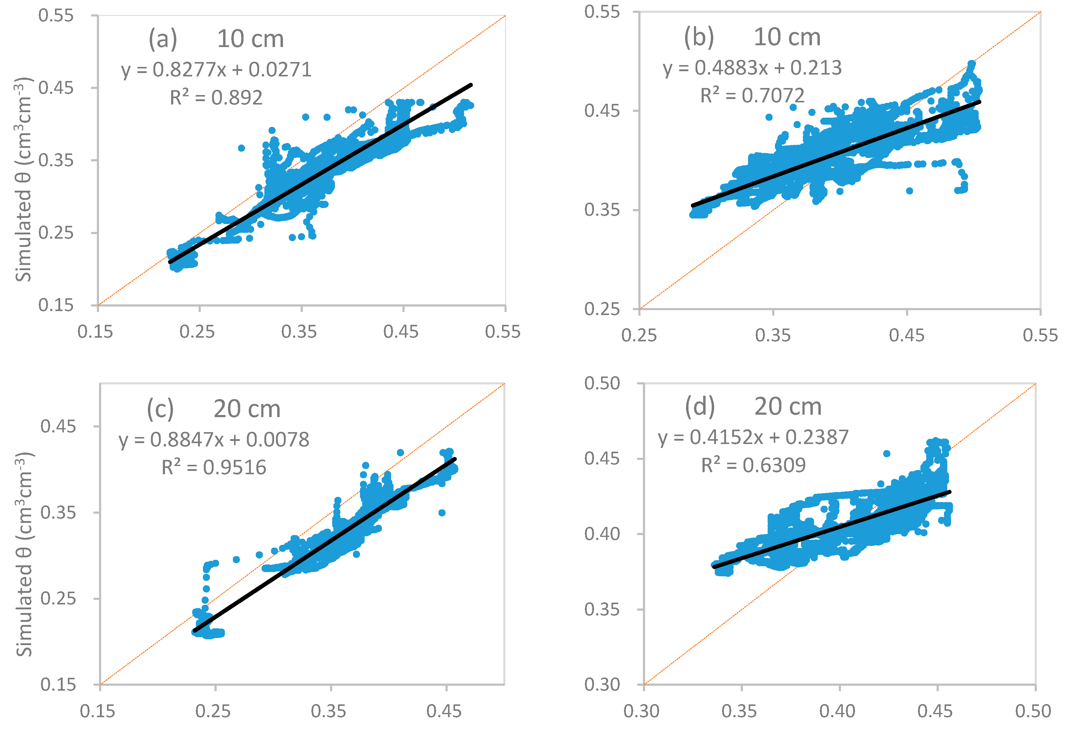
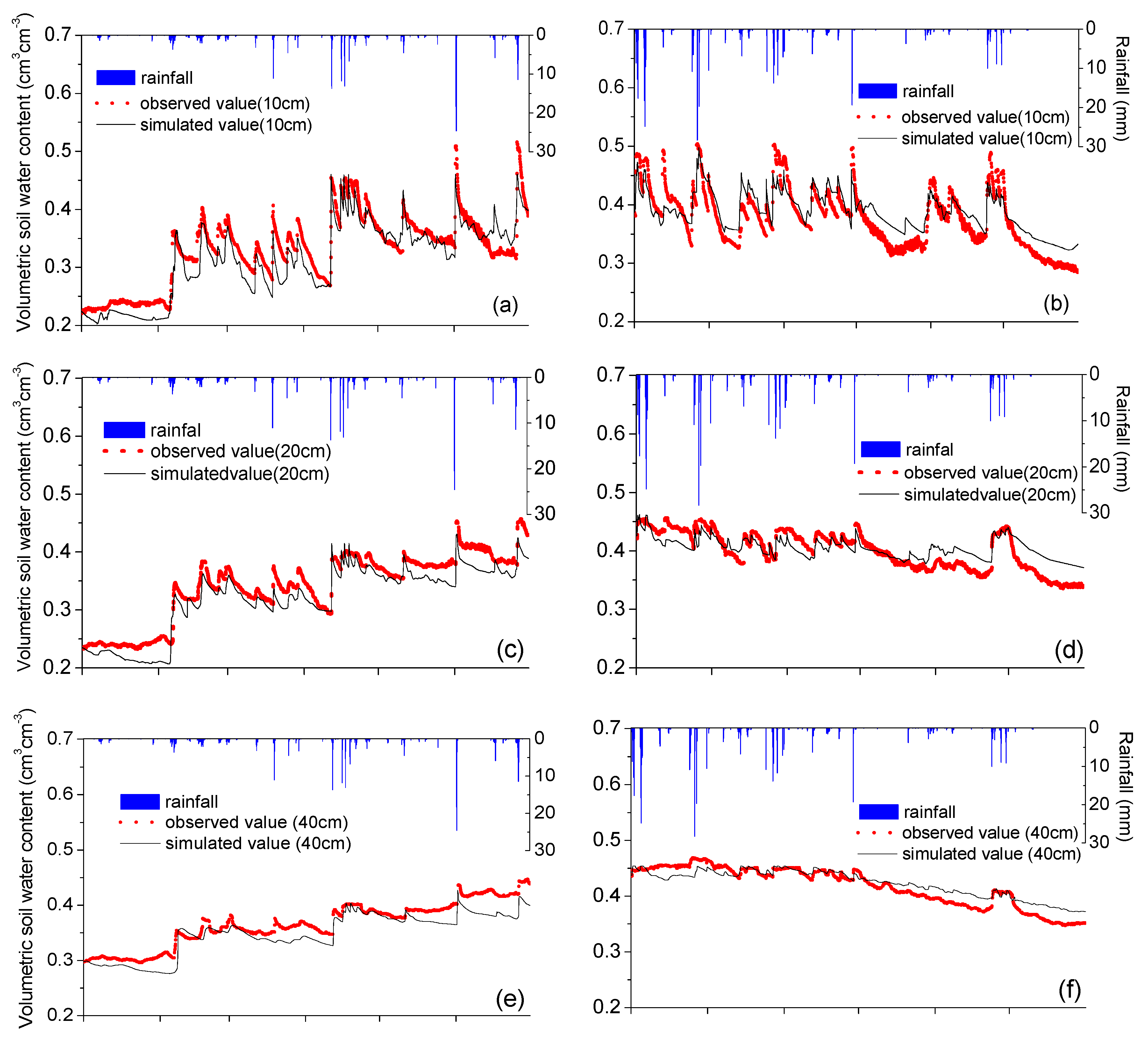
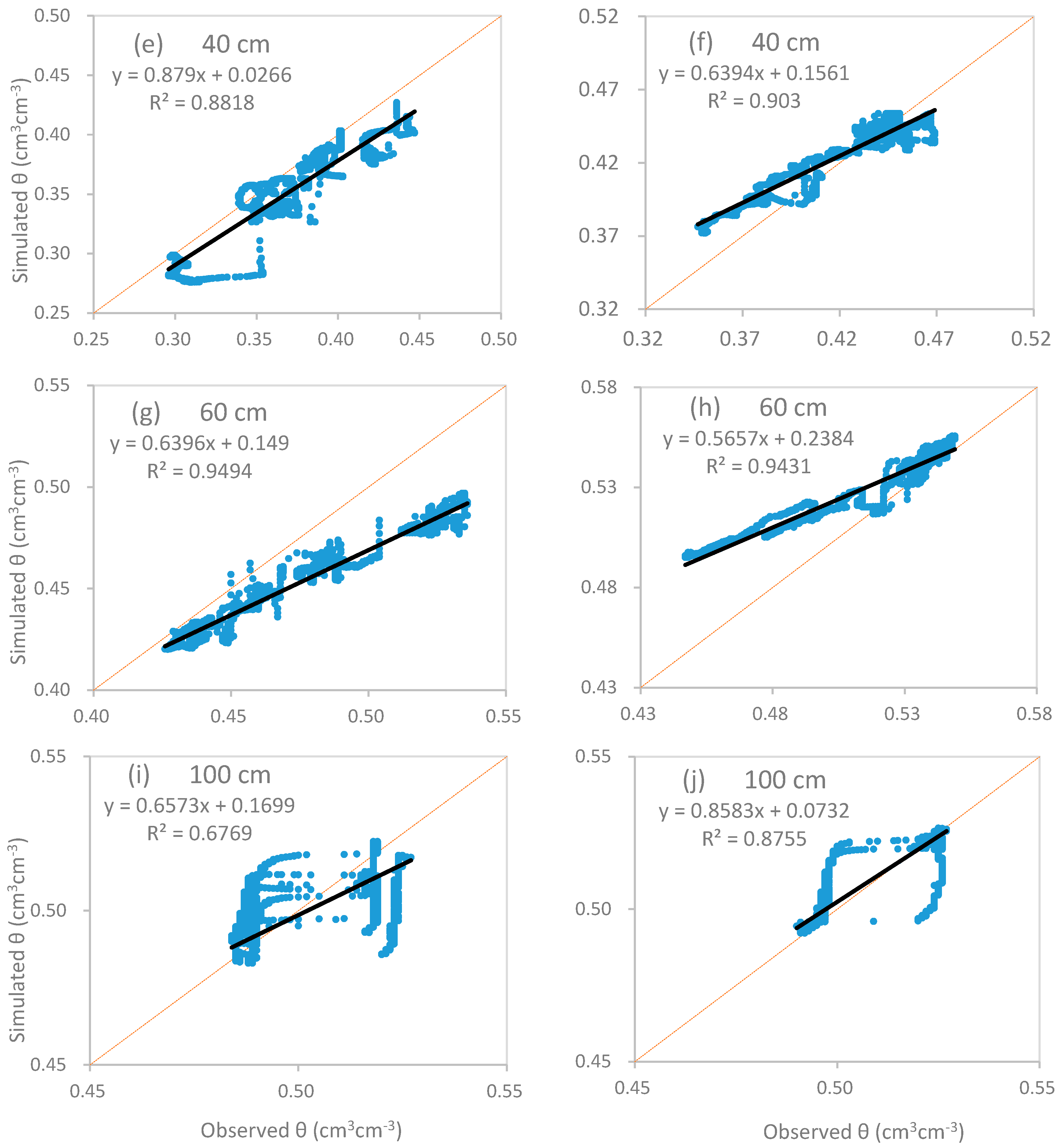
The parameters θr, θs, α, n, Ks and l at the study site were finally identified by calibration and the results are shown in Table 4. To illustrate the performance of the model, comparisons between the simulated and observed values of the soil water content at five depths from 1 January to 30 June 2014 are shown in Figure 6. The agreement of the results is indicated by the relatively large values of R2 and the comparatively small values of RE and RMSE, which are listed in Figure 7 and Table 5.
The model provided good simulations of hourly soil water content compared to the hourly soil water sensor measurements with relatively small RMSE values that were less than 0.05 and comparatively large R2 values of more than 0.6. The values of RE at depths less than 20 cm were over 9%, which were much bigger than those below a 40 cm depth. These discrepancies may be related to uncertainties in the estimation of potential evapotranspiration, which was calculated using pan evaporation data measured out of the experimental field. Additionally, the runoff and discharge in the field deserve further investigation to improve the simulation results [61].
The observed soil water contents increased and decreased more slowly than the simulated values after most rainfall events in the upper layers of soil, while a contrary relationship appeared in the deeper soil layers. A tendency of overall increasing of soil water contents from winter to summer was more obvious in the measurements than simulation. These may be caused by the shallow groundwater table in the field being connected to the water table of the whole plain. Many influential factors can make the shallow groundwater table change out of the control of the direct atmospheric boundary such as irrigations for huge regions of farmland and irregular precipitation in space and time [20,53].
The previously calibrated model was further validated based on the observation data from 1 July to 31 December 2014, using the measured soil volumetric water contents of different soil layers at depths of 10 cm, 20 cm, 40 cm, 60 cm and 100 cm to construct the initial condition. Results are shown in Figure 6. On the whole, the simulated results were close to the observations, especially for the soil water contents in deep soil. The average RMSE and RE values of the soil water content at the five depths were 0.0192 cm3·cm−3 and 2.09%, respectively. The coefficient of correlation (R2 = 0.8119) showed an acceptable correlation between the measured and simulated hourly soil water contents. As indicated in Figure 6, the modeling simulation slightly overestimated the soil water contents at soil depths less than 100 cm, which was the opposite of calibration results. This difference may be caused by the seasonal changes as the observations from summer to winter had the opposite tendency of those from winter to summer, being affected by seasonal variations of several meteorological elements. Moreover, the shallow groundwater table in the study site is controlled by the water table of the whole area and is influenced by anthropogenic recharge and discharge and the temporal and spatial variations of rainfall. Therefore, further investigation will take the problems of a series of uncertain factors and scale in consideration to illustrate the changes in soil water content and improve the model [62,63,64].
4. Conclusions
Soil water is a determinant part in the interaction between surface water and groundwater, both of which are important for crop growth and for farm planning decisions. Furthermore, it affects flood risk mitigation and increases in productivity.
In the present study, to research the temporal and vertical change rule of soil water contents as a typical example for delta plains, two approaches were combined: First, a special experimental field was set up in a delta plain and targeted observations for soil water content were conducted where a series of analyses of soil water content data indicated that soils in this field were wetted to the degree of saturation from 26.6–56.3% and the maximum soil water contents varied at different depths. The capillary action was significant in this region and the height of this capillary rise could be quite substantial and the soil water contents at depths of more than 100 cm could obtain enough recharge from the groundwater to remain fairly constant. Second, a simplified 3D soil water numerical model, especially for delta plains was built, which treated the complete subsurface space as a unified whole and the soil water in the unsaturated zone was integrated with the saturated flow. The simulation results were close to the field observations and followed short-term responses to hydrological events, although the longer-term seasonal trend needed to be improved. The results indicated that the model could be used to calculate soil water content in three dimensions based on the given rainfall data, especially for where the capillary rise of the soil is significant. Temporal and spatial expansion should be the orientation of future research activities. The model should be further improved for long-term simulation suitability and be applied in basin scale.
Acknowledgments
This research is supported by the National Key R&D Programme of China (2016YFA0601000), the Postgraduate Research & Practice Innovation Program of Jiangsu Province (KYCX17_0411), the state major project of water pollution control and management (2014ZX07101-011), the Fundamental Research Funds for the Central Universities (2017B608X14 and 2017B05814) and Jiangsu water conservancy science and technology project (SLT-KY-2015007). We also wish to thank the students who contributed to the field work including Shipeng Du, Liguo Zhu and Jingbo Chen.
Author Contributions
The field work was conducted by Wenjuan Hua, Chuanhai Wang, Hai Yang and Yue Zhai; the paper was written by Wenjuan Hua; Chuanhai Wang and Gang Chen reviewed and improved the manuscript with comments; and the data compilation and statistical analyses were completed by all authors.
Conflicts of Interest
The authors declare no conflict of interest.
References
- Brauer, C.C.; Teuling, A.J.; Torfs, P.J.J.F.; Uijlenhoet, R. The wageningen lowland runoff simulator (walrus): A lumped rainfall-runoff model for catchments with shallow groundwater. Geosci. Model Dev. 2014, 7, 2313–2332. [Google Scholar] [CrossRef] [Green Version]
- Yan, R.; Gao, J.; Dong, C.; Huang, J. Assessment of ecosystem services for polder terrestrial ecosystem in the Taihu Basin. Res. Environ. Sci. 2015, 28, 393–400. [Google Scholar]
- Wandee, P. Optimization of Water Management in Polder Areas: Some Examples for the Temperate Humid and the Humid Tropical Zone. Ph.D. Thesis, Wageningen University, Wageningen, The Netherlands, 2005. [Google Scholar]
- Koch, S.; Bauwe, A.; Lennartz, B. Application of the swat model for a tile-drained lowland catchment in north-eastern Germany on subbasin scale. Water Resour. Manag. 2013, 27, 791–805. [Google Scholar] [CrossRef]
- Northcott, W.J.; Cooke, R.A.; Walker, S.E.; Mitchell, J.K.; Hirschi, M.C. Modeling flow on tile-drained watershed using a GIS-integrated DRAINMOD. Trans. ASAE 2002, 45, 1405–1423. [Google Scholar] [CrossRef]
- Vereecken, H.; Huisman, J.A.; Pachepsky, Y.; Montzka, C.; Kruk, J.V.D.; Bogena, H.; Weihermüllera, M.; Herbsta, M.; Martinezb, G.; Vanderborghta, J.; et al. On the spatio-temporal dynamics of soil moisture at the field scale. J. Hydrol. 2014, 516, 76–96. [Google Scholar] [CrossRef]
- Cornelissen, T.; Diekkrüger, B.; Bogena, H.R. Significance of scale and lower boundary condition in the 3D simulation of hydrological processes and soil moisture variability in a forested headwater catchment. J. Hydrol. 2014, 516, 140–153. [Google Scholar] [CrossRef]
- Romano, N. Soil moisture at local scale: Measurements and simulations. J. Hydrol. 2014, 516, 6–20. [Google Scholar] [CrossRef]
- Servadio, P. Applications of empirical methods in central Italy for predicting field wheeled and tracked vehicle performance. Soil Tillage Res. 2010, 110, 236–242. [Google Scholar] [CrossRef]
- Servadio, P.; Bergonzoli, S.; Beni, C. Soil tillage systems and wheat yield under climate change scenarios. Agronomy 2016, 6, 43. [Google Scholar] [CrossRef]
- Western, A.W.; Zhou, S.L.; Grayson, R.B.; McMahon, T.A.; Blöschl, G.; Wilson, D.J. Spatial correlation of soil moisture in small catchments and its relationship to dominant spatial hydrological processes. J. Hydrol. 2004, 286, 113–134. [Google Scholar] [CrossRef]
- Schwärzel, K.; Menzer, A.; Clausnitzer, F.; Spank, U.; Häntzschel, J.; Grünwald, T.; Köstner, B.; Bernhofer, C.; Feger, K.H. Soil water content measurements deliver reliable estimates of water fluxes: A comparative study in a beech and a spruce stand in the Tharandt forest (Saxony, Germany). Agric. For. Meteorol. 2009, 149, 1994–2006. [Google Scholar] [CrossRef]
- Schume, H.; Jost, G.; Hager, H. Soil water depletion and recharge patterns in mixed and pure forest stands of European beech and Norway spruce. J. Hydrol. 2004, 289, 258–274. [Google Scholar] [CrossRef]
- Jost, G.; Schume, H.; Hager, H. Factors controlling soil water-recharge in a mixed European beech (Fagus sylvatica L.)–Norway spruce [Picea abies (L.) Karst.] stand. Eur. J. For. Res. 2004, 123, 93–104. [Google Scholar] [CrossRef]
- Grayson, R.B.; Western, A.W.; Chiew, F.H.S.; Böschl, G. Preferred states in spatial soil moisture patterns: Local and nonlocal controls. Water Resour. Res. 1997, 33, 2897–2908. [Google Scholar] [CrossRef]
- Vereecken, H.; Kamai, T.; Harter, T.; Kasteel, R.; Hopmans, J.; Vanderborght, J. Explaining soil moisture variability as a function of mean soil moisture: A stochastic unsaturated flow perspective. Geophys. Res. Lett. 2007, 34, 315–324. [Google Scholar] [CrossRef]
- Beni, C.; Servadio, P.; Marconi, S.; Neri, U.; Aromolo, R.; Diana, G. Anaerobic digestate administration: Effect on soil physical and mechanical behavior. Commun. Soil Sci. Plant Anal. 2012, 43, 821–834. [Google Scholar] [CrossRef]
- Pan, F.; Peters-Lidard, C.D. On the relationship between mean and variance of soil moisture fields. J. Am. Water Resour. Assoc. 2008, 44, 235–242. [Google Scholar] [CrossRef]
- Ivanov, V.Y.; Fatichi, S.; Jenerette, G.D.; Espeleta, J.F.; Troch, P.A.; Huxman, T.E. Hysteresis of soil moisture spatial heterogeneity and the ‘‘homogenizing’’ effect of vegetation. Water Resour. Res. 2010, 46. [Google Scholar] [CrossRef]
- Rosenbaum, U.; Bogena, H.R.; Herbst, M.; Huisman, J.A.; Peterson, T.J.; Weuthen, A.; Western, A.W.; Vereecken, H. Seasonal and event dynamics of spatial soil moisture patterns at the small catchment scale. Water Resour. Res. 2012, 48, 3472–3476. [Google Scholar] [CrossRef]
- Servadio, P.; Bergonzoli, S.; Verotti, M. Delineation of management zones based on soil mechanical-chemical properties to apply variable rates of inputs throughout a field (VRA). Eng. Agric. Environ. Food 2017, 10, 20–30. [Google Scholar] [CrossRef]
- Motz, L.H.; Dogan, A. Saturated-unsaturated 3D Groundwater Model. I: Development. J. Hydrol. Eng. 2005, 10, 492–504. [Google Scholar]
- Fares, A.; Temimi, M.; Morgan, K.; Kelleners, T.J. In-situ and remote soil moisture sensing technologies for vadose zone hydrology. Vadose Zone J. 2013, 12, 332–338. [Google Scholar] [CrossRef]
- Robinson, D.A.; Binley, A.; Crook, N.; Day-Lewis, F.D.; Ferré, T.P.A.; Grauch, V.J.S.; Knight, R.; Knoll, M.; Lakshmi, V.; Miller, R.; et al. Advancing process-based watershed hydrological research using near-surface geophysics: A vision for and review of, electrical and magnetic geophysical methods. Hydrol. Process. 2008, 22, 3604–3635. [Google Scholar] [CrossRef]
- Robinson, D.A.; Campbell, C.S.; Hopmans, J.W.; Hornbuckle, B.K.; Jones, S.B.; Knight, R.; Ogden, F.; Selker, J.; Wendroth, O. Soil moisture measurement for ecological and hydrological watershed-scale observatories: A review. Vadose Zone J. 2008, 7, 358–389. [Google Scholar] [CrossRef]
- Vereecken, H.; Huisman, J.A.; Bogena, H.; Vanderborght, J.; Vrugt, J.A.; Hopmans, J.W. On the value of soil moisture measurements in vadose zone hydrology: A review. Water Resour. Res. 2008, 44, 253–270. [Google Scholar] [CrossRef]
- Seneviratne, S.I.; Corti, T.; Davin, E.L.; Hirschi, M.; Jaeger, E.B.; Lehner, I.; Orlowsky, B.; Teuling, A.J. Investigating soil moisture–climate interactions in a changing climate: A review. Earth Sci. Rev. 2010, 99, 125–161. [Google Scholar] [CrossRef]
- Zhu, Q.; Liao, K.; Xu, Y.; Yang, G.; Wu, S.; Zhou, S. Monitoring and prediction of soil moisture spatial-temporal variations from a hydropedological perspective: A review. Soil Res. 2012, 50, 625–637. [Google Scholar] [CrossRef]
- Topp, G.C.; Davis, J.L.; Annan, A.P. Electromagnetic determination of soil water content: Measurements in coaxial transmission lines. Water Resour. Res. 1980, 16, 574–582. [Google Scholar] [CrossRef]
- Simunek, J.; Sejna, M.; van Genuchten, M.T. The HYDRUS-1D software package for simulating the one-dimensional movement of water, heat and multiple solutes in variably-saturated media. In Version 4.0. HYDRUS; University of California Riverside: Riverside, CA, USA, 2008. [Google Scholar]
- Šimunek, J.; Genuchten, M.T.V.; Šejna, M. Recent developments and applications of the HYDRUS computer software packages. Vadose Zone J. 2016, 6. [Google Scholar] [CrossRef]
- Dash, C.J.; Sarangi, A.; Singh, D.K.; Singh, A.K.; Adhikary, P.P. Prediction of root zone water and nitrogen balance in an irrigated rice field using a simulation model. Paddy Water Environ. 2015, 13, 281–290. [Google Scholar] [CrossRef]
- Garg, K.K.; Das, B.S.; Safeeq, M.; Bhadoria, P.B.S. Measurement and modeling of soil water regime in a lowland paddy field showing preferential transport. Agric. Water Manag. 2009, 96, 1705–1714. [Google Scholar] [CrossRef]
- Sander, T.; Gerke, H. Modelling field-data of preferential flow in paddy soil induced by earthworm burrows. J. Contam. Hydrol. 2009, 104, 126–136. [Google Scholar] [CrossRef] [PubMed]
- Tan, X.; Shao, D.; Liu, H. Simulating soil water regime in lowland paddy fields under different water managements using HYDRUS-1D. Agric. Water Manag. 2014, 132, 69–78. [Google Scholar] [CrossRef]
- Rühle, F.A.; Klier, C.; Stumpp, C. Changes in water flow and solute transport pathways during long-term column experiments. Vadose Zone J. 2013, 12, 918–924. [Google Scholar] [CrossRef]
- Rühle, F.A.; Netzer, F.V.; Lueders, T.; Stumpp, C. Response of transport parameters and sediment microbiota to water table fluctuations in laboratory columns. Vadose Zone J. 2015, 10, 1623–1636. [Google Scholar] [CrossRef]
- Yakirevich, A.; Gish, T.J.; Imunek, J.; Genuchten, M.T.V.; Pachepsky, Y.A.; Nicholson, T.J.; Cady, R.E. Potential impact of a seepage face on solute transport to a pumping well. Vadose Zone J. 2010, 9, 686–698. [Google Scholar] [CrossRef]
- Pachepsky, Y.A.; Guber, A.K.; Yakirevich, A.M.; Mckee, L.; Cady, R.E.; Nicholson, T.J. Scaling and pedotransfer in numerical simulations of flow and transport in soils. Vadose Zone J. 2014, 13. [Google Scholar] [CrossRef]
- Šimunek, J.; Van Genuchten, M.T.; Šejna, M. HYDRUS: Model use, calibration and validation. Trans. ASABE 2012, 55, 1561–1574. [Google Scholar]
- Morbidelli, R.; Saltalippi, C.; Flammini, A.; Rossi, E.; Corradini, C. Soil water content vertical profiles under natural conditions: Matching of experiments and simulations by a conceptual model. Hydrol. Process. 2013, 28, 4732–4742. [Google Scholar] [CrossRef]
- Sophocleous, M.A.; Koelliker, J.K.; Govindaraju, R.S.; Birdie, T.; Ramireddygari, S.R.; Perkins, S.P. Integrated numerical modeling for basin-wide water management: The case of the rattlesnake creek basin in south-central Kansas. J. Hydrol. 1999, 214, 179–196. [Google Scholar] [CrossRef]
- Zhang, B.; Lerner, D.N. Modeling of ground water flow to adits. Groundwater 2010, 38, 99–105. [Google Scholar] [CrossRef]
- Labolle, E.M.; Ahmed, A.A.; Fogg, G.E. Review of the integrated groundwater and surface-water model (IGSM). Groundwater 2003, 41, 238–246. [Google Scholar] [CrossRef]
- Demetriou, C.; Punthakey, J.F. Evaluating sustainable groundwater management options using the mike she integrated hydrogeological modelling package. Environ. Model. Softw. 1998, 14, 129–140. [Google Scholar] [CrossRef]
- Narasimhan, T.N. Something to think about … Darcy-Buckingham’s law. Groundwater 1998, 36, 194–195. [Google Scholar] [CrossRef]
- Celia, M.A.; Bouloutas, E.T.; Zarba, R.L. A general mass-conservative numerical solution for the unsaturated flow equation. Water Resour. Res. 1990, 26, 1483–1496. [Google Scholar] [CrossRef]
- Genuchten, M.T.V.; Nielsen, D.R. On describing and predicting the hydraulic properties of unsaturated soil. Ann. Geophys. 1985, 3, 615–628. [Google Scholar]
- Paniconi, C.; Aldama, A.A.; Wood, E.F. Numerical evaluation of iterative and noniterative methods for the solution of the nonlinear Richards equation. Water Resour. Res. 1991, 27, 1147–1163. [Google Scholar] [CrossRef]
- Fares, A. Environmental Impact of Unharvested Forest Buffer Zones upon Cypress-Pond System in Coastal Plains Regions: Modeling Analyses. Ph.D. Thesis, University of Florida, Gainesville, FL, USA, 1996. [Google Scholar]
- Hou, L.; Wang, X.S.; Hu, B.X.; Shang, J.; Wan, L. Experimental and numerical investigations of soil water balance at the hinterland of the Badain Jaran Desert for groundwater recharge estimation. J. Hydrol. 2016, 540, 386–396. [Google Scholar] [CrossRef]
- Schwen, A.; Bodner, G.; Loiskandl, W. Time-variable soil hydraulic properties in near-surface soil water simulations for different tillage methods. Agric. Water Manag. 2011, 99, 42–50. [Google Scholar] [CrossRef]
- Geris, J.; Tetzlaff, D.; Mcdonnell, J.J.; Soulsby, C. Spatial and temporal patterns of soil water storage and vegetation water use in humid northern catchments. Sci. Total Environ. 2017, 595, 486–493. [Google Scholar] [CrossRef] [PubMed]
- Schindler, U.; Müller, L.; Behrendt, A. Field investigations of soil hydrological properties of fen soils in North-East Germany. J. Plant Nutr. Soil Sci. 2003, 166, 364–369. [Google Scholar] [CrossRef]
- García, G.M.; Pachepsky, Y.A.; Vereecken, H. Effect of soil hydraulic properties on the relationship between the spatial mean and variability of soil moisture. J. Hydrol. 2014, 516, 154–160. [Google Scholar] [CrossRef]
- Wang, N.Q.; Wang, Q.T.; Liu, X.L.; Pang, Q. Prediction study of capillary rise height on unsaturated soil. Adv. Mater. Res. 2013, 860–863, 1260–1264. [Google Scholar] [CrossRef]
- Al-Samahiji, D.; Houston, S.; Houston, W. Degree and extent of wetting due to capillary rise in soils. Transp. Res. Rec. 2000, 1709, 114–120. [Google Scholar] [CrossRef]
- Amer, A.M. Water flow and conductivity into capillary and non-capillary pores of soils. J. Soil Sci. Plant Nutr. 2012, 12, 99–112. [Google Scholar] [CrossRef]
- Huza, J.; Teuling, A.J.; Braud, I.; Grazioli, J.; Melsen, L.A.; Nord, G.; Raupach, T.H.; Uijlenhoet, R. Precipitation, soil moisture and runoff variability in a small river catchment (Ardèche, France) during hymex special observation period 1. J. Hydrol. 2014, 516, 330–342. [Google Scholar] [CrossRef] [Green Version]
- Lin, G.; Wang, T.; Zheng, X. Assessing effects of soil hydraulic properties on the temporal stability of absolute soil moisture content and soil moisture anomaly under different climatic conditions. Environ. Earth Sci. 2016, 75, 143. [Google Scholar] [CrossRef]
- Brocca, L.; Ciabatta, L.; Massari, C.; Camici, S.; Tarpanelli, A. Soil moisture for hydrological applications: Open questions and new opportunities. Water 2017, 9, 140. [Google Scholar] [CrossRef]
- Dogan, A.; Motz, L.H. Saturated-unsaturated 3D groundwater model. II: Verification and application. J. Hydrol. Eng. 2005, 10, 505–515. [Google Scholar] [CrossRef]
- Porporato, A.; Daly, E.; Rodrigueziturbe, I. Soil water balance and ecosystem response to climate change. Am. Nat. 2004, 164, 625–632. [Google Scholar] [CrossRef] [PubMed]
- Ojha, R.; Morbidelli, R.; Saltalippi, C.; Flammini, A.; Rao, S.G. Scaling of surface soil moisture over heterogeneous fields subjected to a single rainfall event. J. Hydrol. 2014, 516, 21–36. [Google Scholar] [CrossRef]
Figure 1.
Field tests: (a) Site of the study in Taihu Basin; (b) layout of the experimental field; and (c) vertical layout of the field (0.0–2.0 m depth).
Figure 1.
Field tests: (a) Site of the study in Taihu Basin; (b) layout of the experimental field; and (c) vertical layout of the field (0.0–2.0 m depth).

Figure 2.
View of the some measuring instruments installed in the experimental field: (a) meteorological station; (b) soil water profile and sensors; (c) groundwater observation well; and (d) HOBO data logger.
Figure 2.
View of the some measuring instruments installed in the experimental field: (a) meteorological station; (b) soil water profile and sensors; (c) groundwater observation well; and (d) HOBO data logger.

Figure 3.
Daily mean temperature (°C), evaporation (mm), rainfall (mm) and volumetric soil water contents (cm3·cm−3) at five depths of soil layers: 10, 20, 40, 60 and 100 cm at the experimental field, from 1 January 2014 to 31 December 2014.
Figure 3.
Daily mean temperature (°C), evaporation (mm), rainfall (mm) and volumetric soil water contents (cm3·cm−3) at five depths of soil layers: 10, 20, 40, 60 and 100 cm at the experimental field, from 1 January 2014 to 31 December 2014.
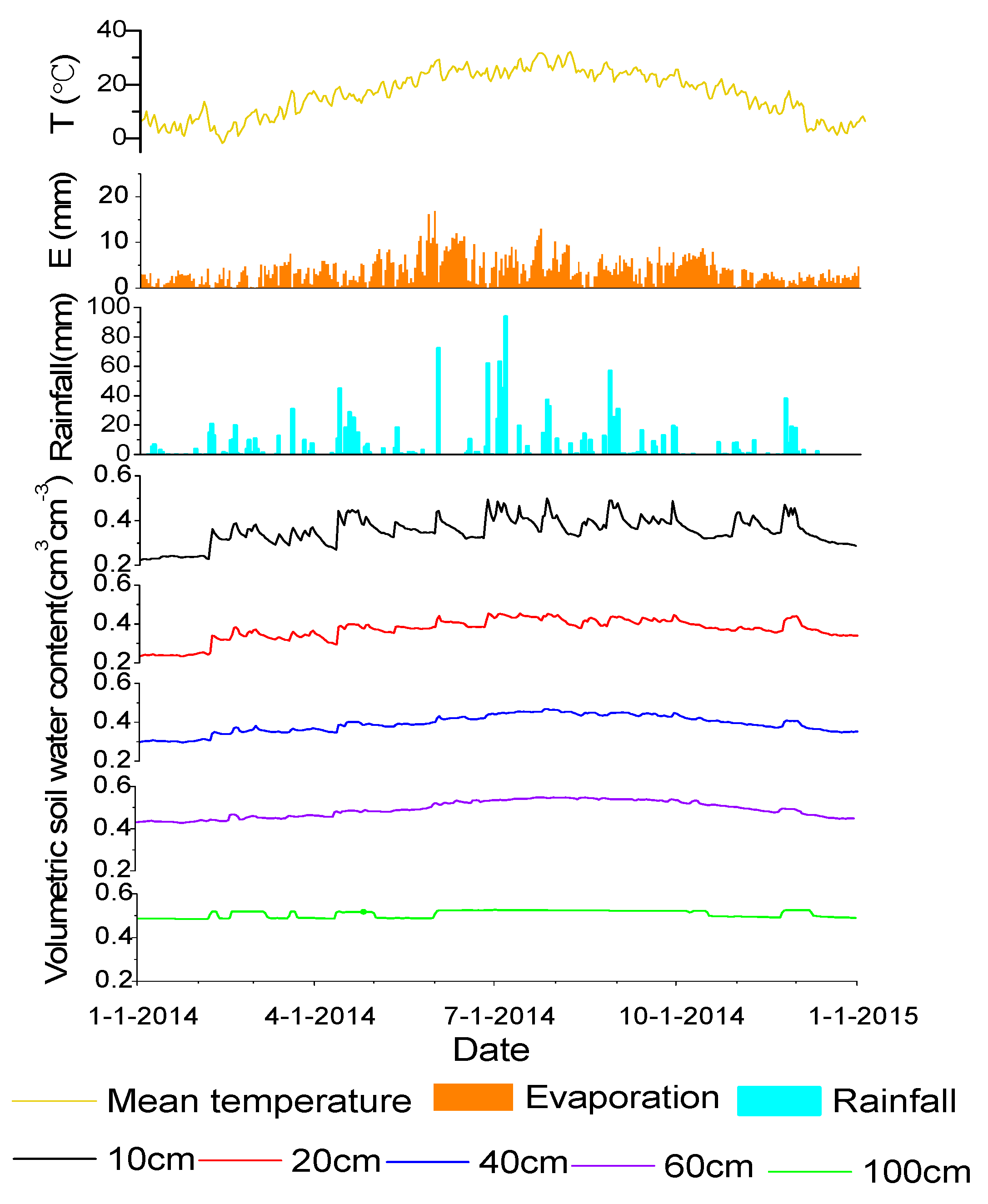
Figure 4.
Soil water content at different depths of a soil profile: (a) during a rainfall event; and (b) during the 12-day evaporation period. Lines B1 to B3, D5 to D30 and A32 to A36 represent the soil water content before, during and after a rainfall event, respectively; the numbers represent the number of hours. Lines Day1 to Day12 show the soil water content from the first day to the twelfth day and the numbers represent the number of days.
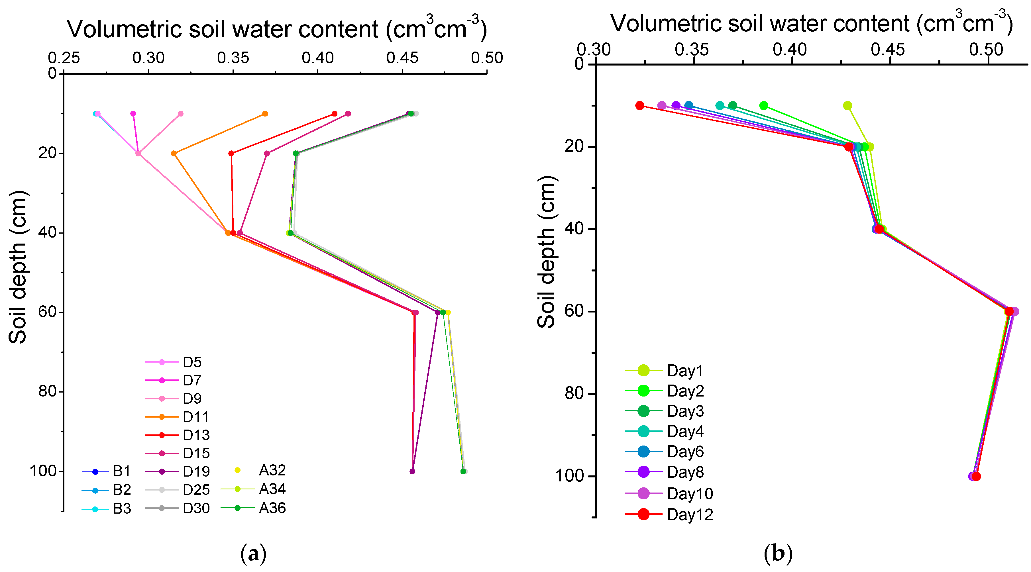
Figure 5.
Rainfall conditions: (a) Shallow water table and soil water contents at 0.10, 0.20, 0.40, 0.60 and 1.00 m soil depths during 2014; (b–f) changes under five different rainfall conditions.
Figure 5.
Rainfall conditions: (a) Shallow water table and soil water contents at 0.10, 0.20, 0.40, 0.60 and 1.00 m soil depths during 2014; (b–f) changes under five different rainfall conditions.
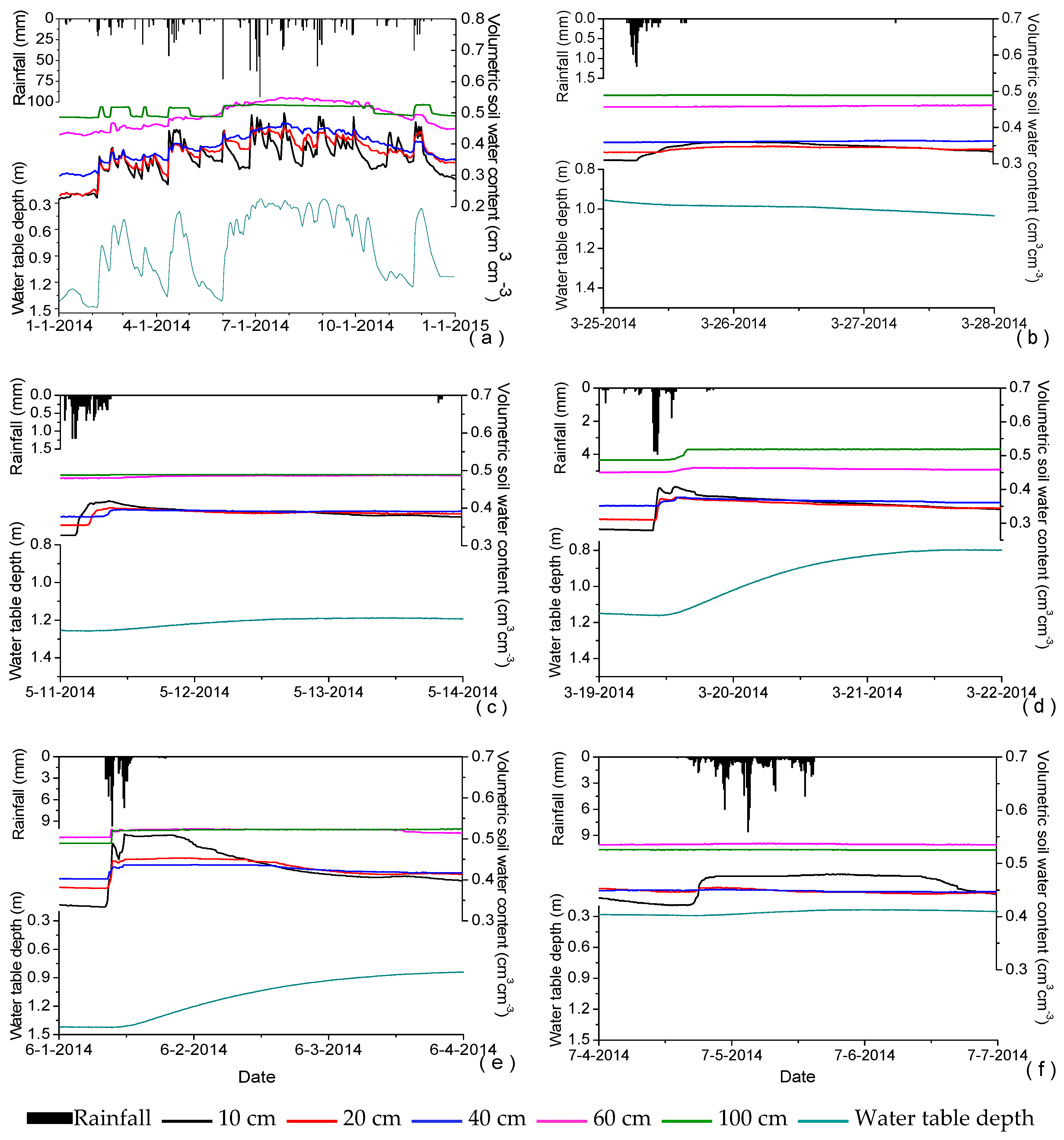
Figure 6.
Simulated results (curves) versus observed (dots) soil water contents at different depths from 1 January 2014 to 30 June 2014 for calibration (a,c,e,g,i) and from 1 July 2014 to 31 December 2014 for validation (b,d,f,h,j). Daily rainfall measurements were also plotted.
Figure 6.
Simulated results (curves) versus observed (dots) soil water contents at different depths from 1 January 2014 to 30 June 2014 for calibration (a,c,e,g,i) and from 1 July 2014 to 31 December 2014 for validation (b,d,f,h,j). Daily rainfall measurements were also plotted.

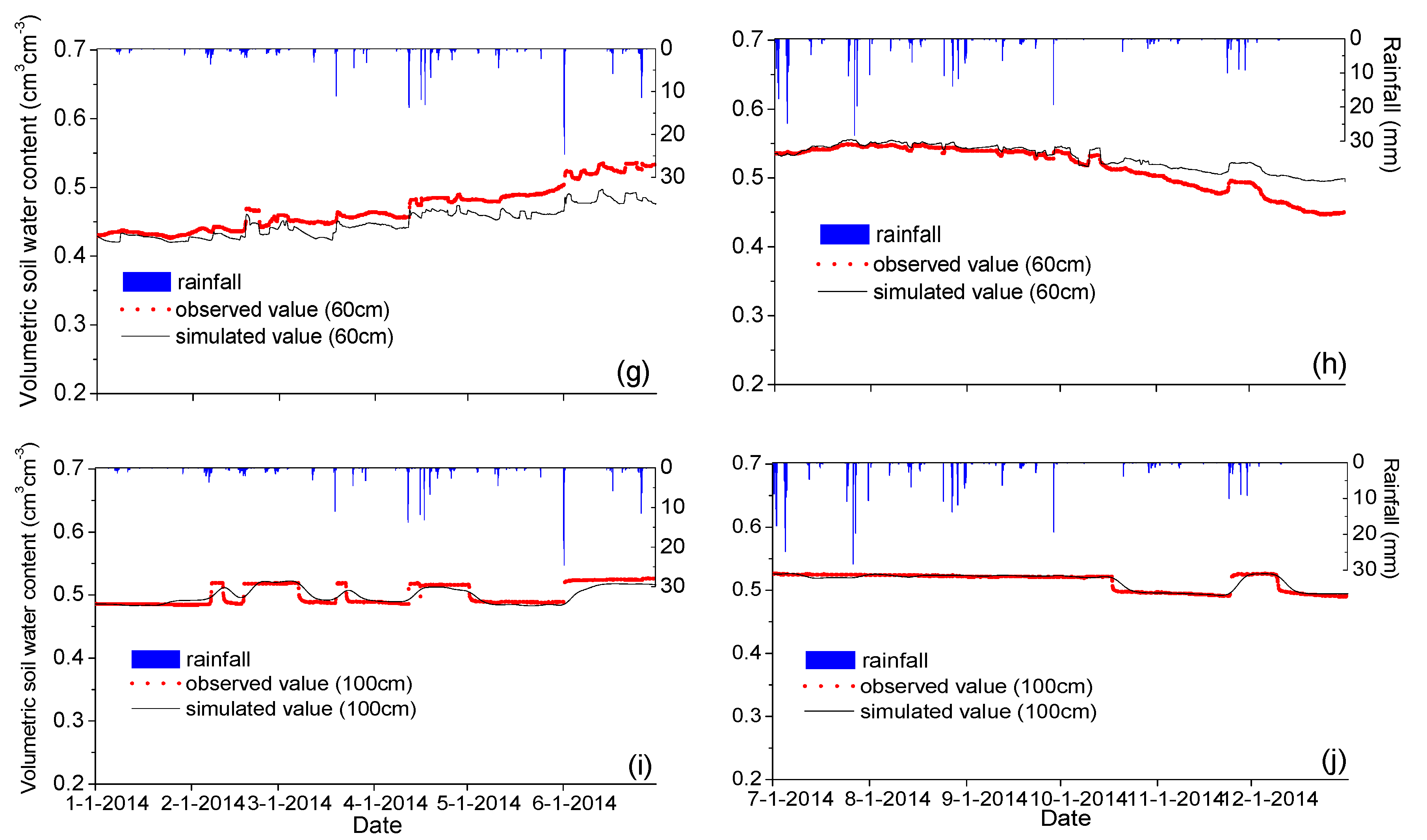
Figure 7.
Correlation of simulated vs. observed volumetric soil water content (θ) at different depths. Results of the calibration (a,c,e,g,i) and validation (b,d,f,h,j) for the model are shown.
Figure 7.
Correlation of simulated vs. observed volumetric soil water content (θ) at different depths. Results of the calibration (a,c,e,g,i) and validation (b,d,f,h,j) for the model are shown.


Table 1.
Physical properties and grain composition of soil samples at different depths in the north, center and south of the experimental field.
Table 1.
Physical properties and grain composition of soil samples at different depths in the north, center and south of the experimental field.
| Soil Sample at Different Depths | Unit Weight (g/cm3) | Saturated Hydraulic Conductivity (10−4 cm/s) | Grain Composition (Particle Diameter) | ||
|---|---|---|---|---|---|
| <0.002 (%) | 0.002–0.05 (%) | >0.05 (%) | |||
| N10 cm | 1.24 | 7.44 | 29.87 | 57.07 | 13.07 |
| N20 cm | 1.13 | 13.08 | 27.20 | 60.80 | 12.00 |
| N40 cm | 1.44 | 17.71 | 27.73 | 65.07 | 7.20 |
| N60 cm | 1.43 | 23.60 | 33.60 | 59.73 | 6.67 |
| N100 cm | 1.48 | 5.24 | 42.13 | 52.80 | 5.07 |
| C10 cm | 1.12 | 21.98 | 30.40 | 58.67 | 10.93 |
| C20 cm | 1.35 | 2.49 | 29.87 | 61.87 | 8.27 |
| C40 cm | 1.50 | 8.89 | 28.80 | 61.33 | 9.87 |
| C60 cm | 1.47 | 14.98 | 33.60 | 61.33 | 5.07 |
| C100 cm | 1.43 | 7.10 | 39.47 | 56.53 | 4.00 |
| S10 cm | 1.24 | 31.11 | 32.00 | 54.40 | 13.60 |
| S20 cm | 1.21 | 22.14 | 30.40 | 60.27 | 9.33 |
| S40 cm | 1.46 | 8.05 | 31.47 | 63.47 | 5.07 |
| S60 cm | 1.47 | 9.27 | 32.00 | 62.40 | 5.60 |
| S100 cm | 1.48 | 1.23 | 40.53 | 53.33 | 6.13 |
Table 2.
Variation of shallow groundwater table under different rainfall conditions.
| Figure 5 | Rainfall Amount (mm) | Rainfall Intensity (mm/h) | Rainfall Duration (mm) | Water Table Depth 1 (m) | Water Table Depth 2 (m) | Water Table Variation (m) |
|---|---|---|---|---|---|---|
| (b) | 9.3 | 1.47 | 6.33 | 0.955 | 1.034 | –0.079 |
| (c) | 17.5 | 2.19 | 8.0 | 1.255 | 1.190 | 0.065 |
| (d) | 30.8 | 6.16 | 5.0 | 1.160 | 0.800 | 0.360 |
| (e) | 72.3 | 16.07 | 4.5 | 1.423 | 0.840 | 0.583 |
| (f) | 138.6 | 5.78 | 24.0 | 0.290 | 0.238 | 0.052 |
Table 3.
Pearson correlation analysis between daily soil water content (θ) and rainfall (P) or water table depth (H) at different soil depths.
Table 3.
Pearson correlation analysis between daily soil water content (θ) and rainfall (P) or water table depth (H) at different soil depths.
| Pearson Correlation Coefficient | ||
|---|---|---|
| Soil Depths(cm) | P-θ | H-θ |
| 10 cm | 0.327 | –0.680 |
| 20 cm | 0.202 | –0.785 |
| 40 cm | 0.179 | –0.811 |
| 60 cm | 0.151 | –0.759 |
| 100 cm | 0.175 | –0.925 |
Table 4.
Calibrated hydraulic parameters for the five soil zones in the model.
| Depth | θr | θs | α (1/cm) | n | Ks (10−4 cm/s) | l |
|---|---|---|---|---|---|---|
| 0~15 cm | 0.10 | 0.46 | 0.013 | 1.48 | 2.6 | 0.5 |
| 15~30 cm | 0.10 | 0.42 | 0.0116 | 1.35 | 1.7 | 0.5 |
| 30~55 cm | 0.10 | 0.42 | 0.009 | 1.38 | 0.8 | 0.5 |
| 55~80 cm | 0.10 | 0.50 | 0.010 | 1.43 | 0.4 | 0.5 |
| 80~200 cm | 0.10 | 0.49 | 0.010 | 1.42 | 0.5 | 0.5 |
Table 5.
The root mean square error (RMSE), mean relative error (RE) and coefficient of correlation (R2) between the simulated and observed soil water contents.
Table 5.
The root mean square error (RMSE), mean relative error (RE) and coefficient of correlation (R2) between the simulated and observed soil water contents.
| Soil Depths (cm) | Volumetric Soil Water Content | |||
|---|---|---|---|---|
| RMSE (cm3·cm−3) | RE (%) | R2 | ||
| Model calibration | 10 | 0.0363 | 9.03 | 0.8920 |
| 20 | 0.0343 | 9.25 | 0.9516 | |
| 40 | 0.0225 | 4.84 | 0.8818 | |
| 60 | 0.0239 | 4.34 | 0.9494 | |
| 100 | 0.0094 | 0.35 | 0.6769 | |
| Model validation | 10 | 0.0348 | 5.13 | 0.7072 |
| 20 | 0.0216 | 1.09 | 0.6309 | |
| 40 | 0.0152 | 1.28 | 0.9030 | |
| 60 | 0.0198 | 2.87 | 0.9431 | |
| 100 | 0.0047 | 0.08 | 0.8755 | |
© 2017 by the authors. Licensee MDPI, Basel, Switzerland. This article is an open access article distributed under the terms and conditions of the Creative Commons Attribution (CC BY) license (http://creativecommons.org/licenses/by/4.0/).
Share and Cite
MDPI and ACS Style
Hua, W.; Wang, C.; Chen, G.; Yang, H.; Zhai, Y. Measurement and Simulation of Soil Water Contents in an Experimental Field in Delta Plain. Water 2017, 9, 947. https://doi.org/10.3390/w9120947
AMA Style
Hua W, Wang C, Chen G, Yang H, Zhai Y. Measurement and Simulation of Soil Water Contents in an Experimental Field in Delta Plain. Water. 2017; 9(12):947. https://doi.org/10.3390/w9120947
Chicago/Turabian StyleHua, Wenjuan, Chuanhai Wang, Gang Chen, Hai Yang, and Yue Zhai. 2017. "Measurement and Simulation of Soil Water Contents in an Experimental Field in Delta Plain" Water 9, no. 12: 947. https://doi.org/10.3390/w9120947
Note that from the first issue of 2016, this journal uses article numbers instead of page numbers. See further details here.