Modeling Stream Bank Erosion: Practical Stream Results and Future Needs


Technical Service Center, U.S. Bureau of Reclamation, Bldg. 67, P.O. Box 25007, Denver, CO 80225, USA
Water 2017, 9(12), 950; https://doi.org/10.3390/w9120950
Submission received: 12 October 2017
/
Revised: 29 November 2017
/
Accepted: 30 November 2017
/
Published: 6 December 2017
(This article belongs to the Special Issue Streambank Erosion: Monitoring, Modeling and Management)
Abstract
:Coupled two-dimensional (2D) morphodynamic and bank erosion models are gaining attentions in recent years. It has been shown that such models have advantages over the one-dimensional (1D) modeling approaches. In this paper, a previous 2D bank erosion model with the moving mesh method is extended to include the fixed mesh approach. Further, two practical streams with differing complexity are simulated to demonstrate the extended model. Both the moving mesh and fixed mesh methods are used in the modeling. The model consists of two components: a 2D flow and mobile-bed model for vertical bed changes and hydraulic forces acting on a bank and a lateral bank retreat model. The 2D vertical model and the lateral bank erosion model are coupled together spatially and temporally through a special procedure and a common mesh. With the experiences gained with practical stream modeling, the modeling procedure and key model input parameters are described. The study shows that the moving and fixed mesh methods together make the extended bank erosion model numerically robust and capable of predicting both the vertical bed changes and the lateral stream bank erosion for complex streams. Each individual method, however, has its own limitations in terms of model accuracy and efficiency. The moving mesh works well if bank retreat is relatively small, e.g., less than one channel width, and produces more accurate results than the fixed mesh method. The fixed mesh may be needed for ensuring numerical stability if a bank may be subject to significant retreat (e.g., more than one channel width). The fixed mesh method, however, is less accurate than the moving mesh method and a much refined mesh may be needed. Both methods need future research and improvements in terms of their model accuracy.
1. Introduction
Stream bank erosion has both benefits and consequences. Bank erosion is important to waterway ecology as bank changes may create a variety of habitats contributing to ecological diversity [1,2]. For this reason, bank protection was removed by some restoration projects [3] and macro-roughness elements such as lateral cavities are added to promote morphological diversity [4]. Bank erosion, however, is mostly detrimental for streams. It causes road collapse and land loss and becomes a significant resource maintenance problem [5]. Accelerated bank erosion can also be a significant point source pollutant [1], presenting challenges to river and reservoir managers. There is a great need to develop reliable and practical numerical models which can be used to understand and predict stream bank erosion in practical streams.
Vertical stream bed erosion has been studied routinely and its modeling is getting wide acceptance [6,7,8]. The same cannot be said with lateral stream bank erosion since both its measurements and numerical modeling are challenging. Simulation of bank erosion requires a numerical model capable of coupling the in-channel vertical erosion processes with the lateral bank erosion processes. Significant effort has been expended in the past on developing numerical models to estimate and/or predict lateral stream bank erosion, but most are for simple cases. Two types of models may be identified [9]: empirical models and process models. Empirical models may be used to estimate equilibrium channel width using either regime equations developed from field data or extremal hypotheses that assume that alluvial channels attain equilibrium when an indicator variable reaches a maximum or minimum. Empirical models may be used for estimating long term changes of channel width and are suitable mostly for dynamically stable channels—they are not the focus of the study. Process models explicitly simulate the physical processes most important for quantifying stream vertical and lateral changes. They may be used to provide short- to medium-term channel changes and are suitable for both stable and unstable streams. The process model is the focus of this study.
A literature review of combined vertical and lateral erosion models has been reported by a number of authors. For example, ASCE [10] provided a review of such models that existed before 1997; Rinaldi and Darby [11] updated this review to include seepage modeling; Langendoen and Simon [12] provided a review focusing primarily on models with geotechnical modeling capabilities; Motta et al. [13] provided a review of models that linearized the 2D governing equations; and Lai [14,15] provided an extensive review of most process models.
A continuous dynamic simulation of combined vertical and lateral erosion has rarely been carried out. Such a simulation requires a vertical mobile-bed model which can provide reliable near-bank fluvial variables used by the lateral bank erosion model. Further, a robust coupling procedure is needed to feed the predicted bank retreat back to the vertical model. One of the early attempts was reported by Mosselman [16] who incorporated the excess bank height concept into the bank erosion model which was then linked to the quasi-steady 2D flow model. This early model simulated equilibrium sediment transport of a single grain size. The model, however, suffered from numerical truncation errors when the mesh became overly skewed, or distorted, and required constant manual rearrangement of the mesh. The model was applied to a reach of the River Ohre, but with poor results. Mosselman [16] attributed the errors to the formulation of the bank erosion mechanism as well as the simplicity of the 2D flow model. Darby et al. [17] incorporated the bank erosion model of Mosselman [16] into an improved 2D depth-averaged model named RIPA. They, however, found that the new coupled model did not significantly improve the previous model of Mosselman [16]. They ascribed this to the systematic under-prediction of transverse bed slope by the flow model and the systematic over-prediction of bank stability by the geotechnical module. Nagata et al. [18] developed a coupled bank erosion research model in which the governing equations were cast in a moving boundary fitted coordinate system along with a new formulation of the non-equilibrium sediment transport. The model was applied to examine the morphological behaviors of experimental channels with good results. Their bank erosion model, however, neglected the difference between basal erosion (a lateral process) and bed degradation (a vertical process). The model is yet to be demonstrated for complex streams. Duan et al. [19] reported a bank erosion research model that integrated a non-cohesive uniform bank module with a 2D vertical model. The rate of bank retreat was linked to the longitudinal gradient of sediment transport, strength of secondary flow and erosion of sediment from the bank. The model was tested with flume cases and found that the simulated meandering wavelength and amplitude did not agree with the observations. A recent bank erosion model was developed by Motta et al. [13] who coupled the bank stability algorithms of Langendoen and Simon [12] to the linearized solutions of the 2D depth-averaged shallow water equations. The approach overcame the need for a migration coefficient to be specified but was strictly valid only for the central region of mildly curved channels in which helical flow could be neglected. The vertical model, however, is not general enough for practical applications.
More general and practical bank erosion models are needed. One such model was reported by Langendoen and Simon [12] who incorporated a comprehensive bank erosion module into a 1D vertical model CONCEPTS (CONservational Channel Evolution and Pollutant Transport System) [20]. The model was applicable to multi-layer cohesive stream banks. The geotechnical algorithm of the model generalized the limit equilibrium method of Simon et al. [21] by employing vertical slices to distribute the weight of the failure block along the failure plane and enabling the automatic detection and insertion of tension cracks. The model was used to simulate the bank retreat of a bendway at the Goodwin Creek, Mississippi. Good agreements were reported in comparison with the measured data after a proper calibration of the bank erodibility coefficient. Following the approach of Langendoen and Simon [12], Lai et al. [22] advanced the combined vertical and lateral bank erosion modeling by incorporating a lateral model into a 2D depth-averaged vertical model. The lateral model was based on the deterministic bank stability and toe erosion model BSTEM [21,23], while the stream vertical changes were predicted with the SRH-2D model [24,25,26]. A robust coupling procedure was developed which minimized the number of model calibration parameters. Satisfactory results were obtained when it was applied to the multi-layer cohesive banks at the Goodwin Creek, Mississippi. In particular, the study found that the use of 2D vertical models improved the bank erosion predictions over the previous 1D modeling of the same site by Langendoen and Simon [12].
Despite much progress over the past decade, a fully coupled vertical and lateral bank erosion model that is generally applicable to practical streams is still elusive. Most models suffer from one or several of the following limitations: (a) use of inflexible meshes to simulate a moving boundary problem; (b) use of steady or quasi-steady flow models; (c) limited consideration of secondary currents that are characteristic of natural meander bends; (d) simplifications to sediment transport and bed deformation sub-models, making them applicable only to idealized cases (e.g., equilibrium transport of single grain sizes); (e) simplistic bank retreat models neglecting key physical processes (e.g., explicitly accounting for only fluvial erosion or mass failure or neither) and requiring a number of “fudge factors” to obtain realistic behaviors; and (f) inappropriate or non-existent coupling procedures. Additionally, most previous efforts have been focused more on the mass failure processes and less on the coupling between the lateral bank processes and the vertical stream processes. Most models lack the demonstration of a continuous dynamic simulation of lateral and vertical processes for practical streams.
An effort in improving the practical side of the bank erosion modeling was reported by Lai [14] in which a simpler bank erosion model was developed besides the more complex, mechanistic failure bank erosion model. This study represents a further advancement by developing a capability into the model of Lai et al. [22] and Lai [14]. Specifically, a fixed mesh approach is developed in lieu of a potential limitation with the moving mesh approach. The revised model removes all limitations in the above list except (f). Our objective is to develop a bank erosion model that is practical, reliable and stable with a minimal set of calibration parameters. Therefore, the revised model is applied to two practical streams. The simulation experience and the results lead to the establishment of the modeling procedure and key model inputs. Lessons learned are also reported along with recommendations for the future needs.
2. Coupled Bank Erosion Model
The coupled vertical and lateral bank erosion model in this study is based on the SRH-2D model developed at the U.S. Bureau of Reclamation as described by Lai et al. [22] and Lai [14]. Readers may refer to those references for further technical details. Herein a summary of the model relevant to this study is provided along with the new fixed mesh approach to handle bank retreat.
2.1. Vertical Erosion
The in-stream vertical fluvial processes are simulated with the 2D depth-averaged hydraulic and sediment transport model SRH-2D. The flow model theory was documented by Lai [24,25]. The model adopts the arbitrarily shaped element method of Lai et al. [26] using the finite-volume discretization and implicit integration scheme. The numerical procedure allows all flow regimes (sub-, super-, and trans-critical flows) simulated simultaneously. The special wetting-drying algorithm makes the model stable to handle the flow over dry surfaces. The vertical erosion module adopts the methodology of Greimann et al. [27] and the theories were described by Lai and Greimann [6] and Lai et al. [7]. The vertical model predicts vertical stream bed changes by tracking multi-size, non-equilibrium sediment transport for suspended, mixed, and bed loads, and for cohesive and non-cohesive sediments, and on granular, erodible rock, or non-erodible beds. The effects of gravity and secondary flows on the sediment transport are accounted for by displacing the direction of the sediment transport vector from that of the local depth-averaged flow vector [6,7].
2.2. Basal Erosion
Basal erosion is the direct removal of bank materials by flowing water in a stream. Several methods may be used to compute basal erosion. In one method, lateral erosion of a bank node is computed using the vertical erosion predicted by the 2D vertical model over a wetted bank. This approach, or its variant, was proposed by Hasegawa [28], and subsequently adopted by Nagata et al. [18], Duan et al. [19], and Chen and Duan [9]. The approach, however, worked well only for special cases; it might incur large uncertainties for steep banks due to limited number of mesh nodes that may be used to represent the banks.
A different approach is adopted in the present study. An arbitrary number of banks may be chosen for the simultaneous modeling of vertical channel processes and lateral bank retreat. Each bank geometry is represented by the toe and top nodes irrespective of the geometry in between. If the fluvial shear stress is known on a bank node, the lateral erosion rate is computed using the following equation e.g., [17,29]:
where εL is lateral erosion rate (m s−1), k is erodibility coefficient (m s−1), τ is shear stress on a bank node (Pa), and τc is critical shear stress (Pa). Two empirical coefficients, critical shear stress and erodibility, are user inputs.
Shear stress distribution along a wetted bank is needed to use Equation (1) but it is not readily available from 2D depth-averaged vertical models (3D models are needed instead). In this study, the linear distribution assumption is adopted. That is, the shear stress is assumed to decrease linearly from bank toe to the intersect point between the bank and water election. The toe shear stress is computed by the 2D vertical model while the shear stress at the intersect point is zero. The linear assumption is appropriate with the present model since the bank has been lumped together as a single unit and only the total amount of eroded bank materials is sought. Uncertainties introduced by the linear assumption may be compensated for through the erodibility coefficient which is to be discussed later.
2.3. Lateral Bank Retreat Rate
The uniform retreat module of Lai [14] is adopted which assumes that the bank is retreating uniformly as a whole without regard to the bank profile details. Mass failure is computed by assuming that a constant bank angle is maintained, such as the angle of repose, and the loss of the bank material equals to the basal erosion. In theory, the uniform bank retreat assumption is strictly valid only for non-cohesive uniform banks with planar failure. It, however, may be applied to other bank types if only the global bank retreat distance, over a specified period, is of interest. More complex process-based bank models, such as those by Langendoen and Simon [12] and Lai [22] are needed if the timing of the bank mass failure or bank face shape is of primary interest. Such complex modeling, however, is still at the research stage and yet to be demonstrated for practical streams [15].
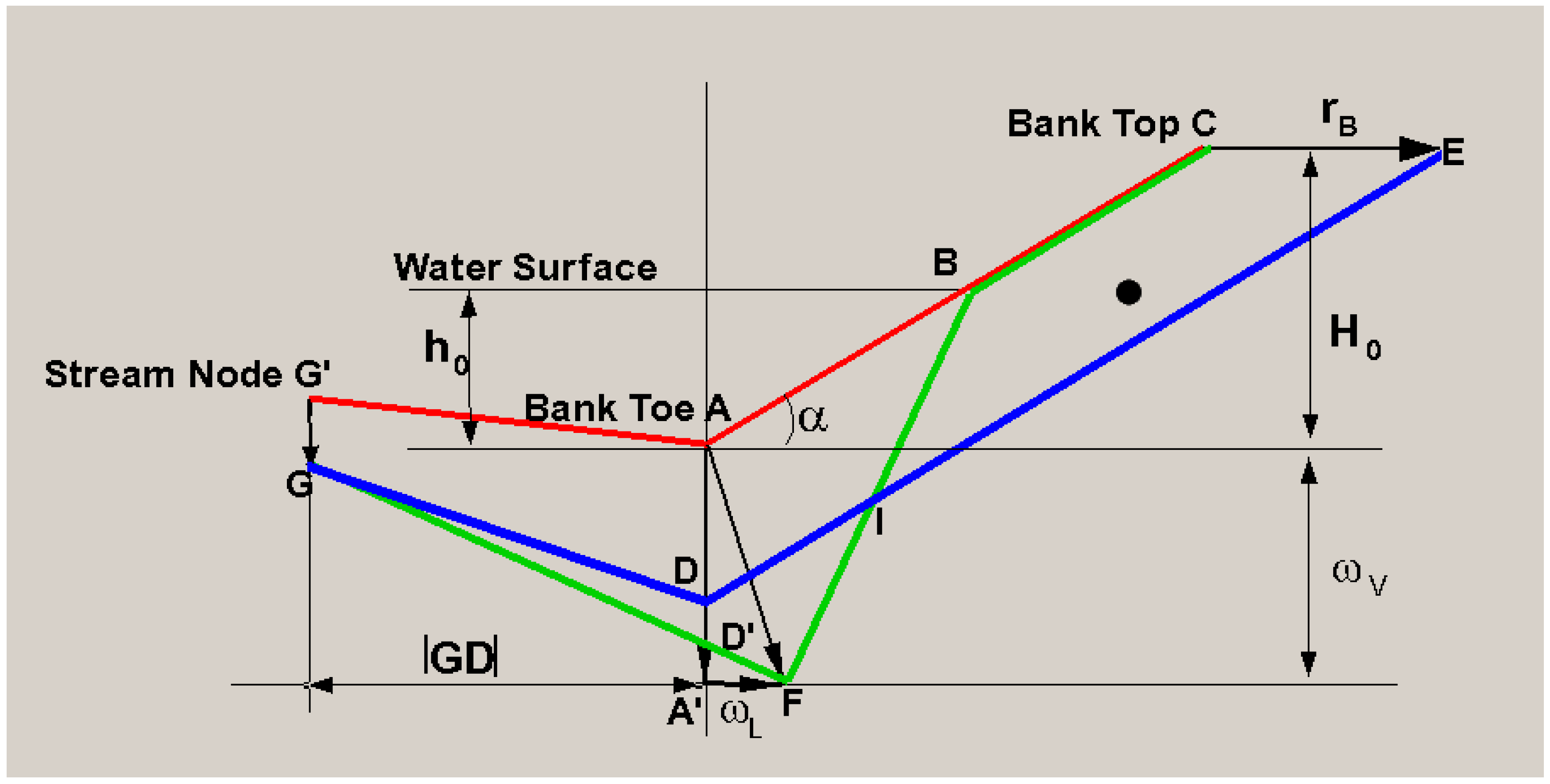
A unique feature of the uniform retreat model is that the bank retreat rate may be derived to give an analytical expression resorting to the mass conservation principle. Its derivation is described herein. Consider a generic bank in Figure 1. The initial bank is G’ABC where G’AB is under water while BC is above and dry. ABC represents the straight bank face at the angle of repose. A is bank toe node, C is bank top, B is the intersect point between the bank and water surface, and G’ is the nearest mesh node to A in the stream. Assume that erosion is occurring: A is eroded vertically to A’ and G’ to G. These vertical erosions are predicted by the 2D vertical model. If the lateral erosion of the toe node is added, A’ would move to point F. The new bank face after basal erosion would be GFBC based on the linear assumption of the shear stress along AB. Now the new bank angle of FB exceeds the angle of repose; therefore, the bank material above B would “fail” to fill the toe area and a final bank face, GDIE, with the angle of repose, would form. The intercept D between the new bank and the vertical line of AA’ may be above or below D’. In Figure 1 and the derivation below, D is assumed to be above D’. Under such a scenario, D is the final toe location. Mass (or area) conservation requires the following to be true (IBCE refers to the area contained within the polygon, etc.):
IBCE = GDIFD’
With some manipulation, the bank retreat distance rB per time step (i.e., distance between C and E) may be computed by the following equation:
In the above, rB is the bank retreat distance (m); h0 is the initial water depth at toe (m); H0 is the initial bank height (m); α is the bank angle or angle of repose (-); ωV is the vertical toe erosion distance predicted by the 2D model (m); ωL is the lateral toe erosion distance computed by equation (m); and |GD| is the horizontal distance between G and D (m).
The bank retreat distance per time step rB under the other scenario of D below D’ may be similarly derived; the final retreat rate expression is the same as Equation (3) by simply setting |GD| = 0. Further, under the scenario of deposition at the bank toe A, the bank would intrude towards the stream. The bank intrusion distance may also be derived similarly; the rate expression is also similar to Equation (3) and they are not repeated. Rate Equation (3) may be viewed as a generalization of Chen and Duan method [9].
2.4. Vertical and Lateral Coupling Procedure
A strategy is needed to couple the lateral bank model with the 2D vertical model. This is probably one of the most important steps in the bank erosion model development as it impacts the stability and ease-of-use of the model for a time accurate dynamic simulation. A general yet simple procedure is described next which facilitates the model application to practical streams.
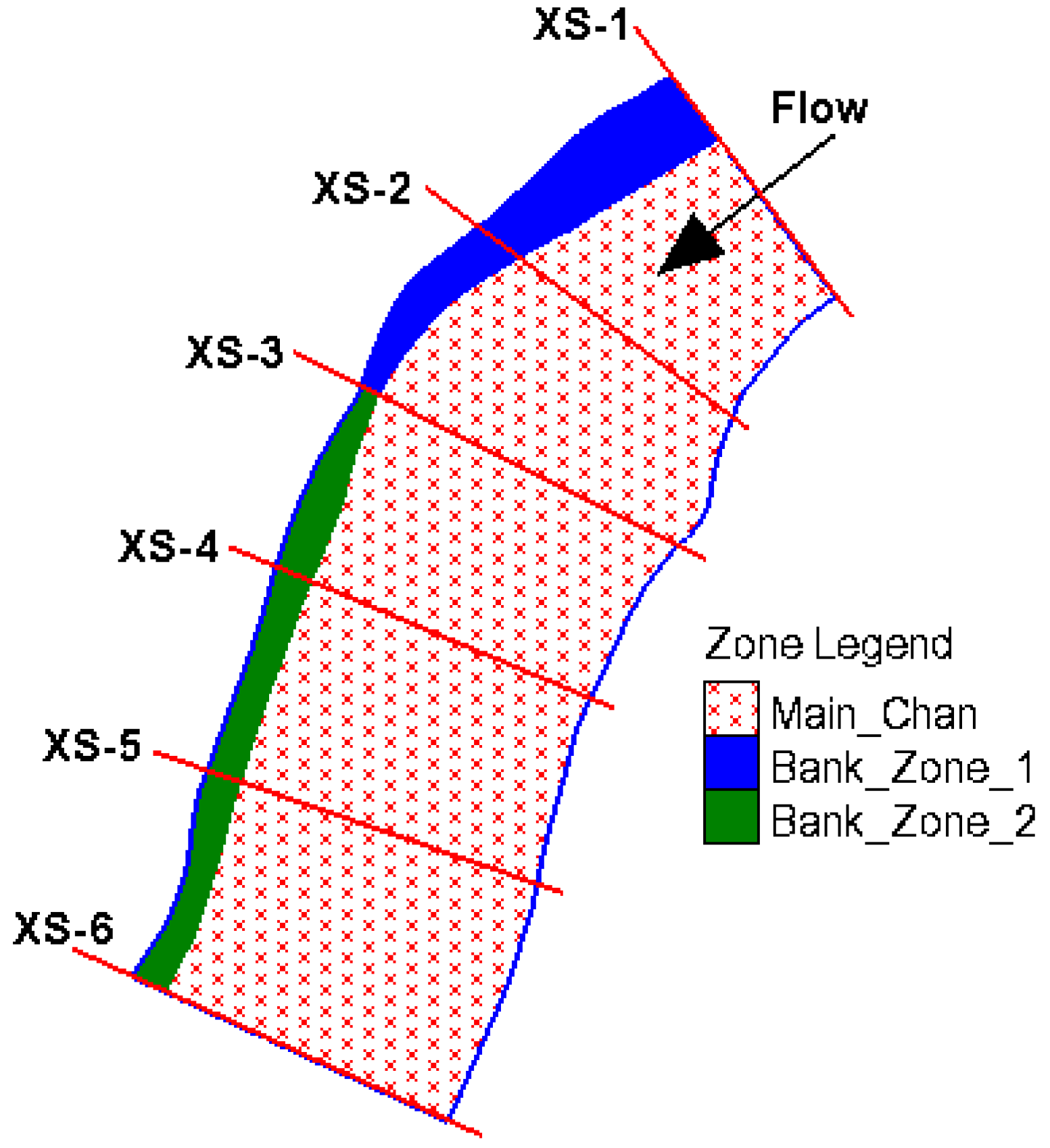
The model setup and inputs for a bank erosion modeling are made the same as a non-bank erosion modeling. An initial 2D mesh is generated along with normal boundary conditions specified. The only extra effort for a bank modeling is that the 2D mesh should have mesh cells representing one or multiple bank zones. A bank zone is used to represents a bank section along which several banks are to be simulated for retreat. As an illustration, Figure 2 shows a sample stream reach whose right bank is to be simulated for bank retreat. Two bank zones are used in the example. Bank zone 1 contains three banks while zone 2 has four banks. Each bank zone is defined by two mesh lines. With the moving mesh approach (to be described next), the two mesh lines represent the bank toe and bank top. With the fixed mesh approach, the two mesh lines represent only the beginning and ending edges of a bank zone.
A key issue is the way to accommodate bank retreat within the 2D mesh during a continuous dynamic simulation. Two approaches are used in this study: the moving mesh and the fixed mesh approaches. The moving mesh approach was described before [14,22]; with this approach, the 2D mesh lines representing the bank toe and top will follow the bank retreat continuously during the dynamic simulation. That is, the 2D mesh is moved and deformed to follow the bank movement. The moving mesh approach has the benefit of a better bank representation and more accurate retreat computation. A drawback is that the 2D mesh has to be re-generated in a dynamic simulation. The mesh regeneration is done automatically for practical model applications; however, the process has the potential to distort the mesh too much to cause model instability. This study shows that the moving mesh approach is the choice if no significant bank retreat is expected (e.g., less than one channel width). In this study, the fixed mesh approach is developed to remove the potential limitations of the moving mesh approach. The fixed mesh approach does not move the mesh during a dynamic simulation. Instead, the moving bank toe and top are represented by fixed mesh nodes at any instance of time through an interpolation procedure. Once the bank toe and top nodes are found associated with mesh nodes, retreat computation may be carried out as described before. The fixed mesh approach removes the mesh distortion issue, but bank toe and top locations are only approximately represented by the mesh. This may lead to high numerical errors if the mesh is coarse. The computed bank retreat errors increase with the mesh size. A much refined mesh may be required to capture the bank retreat reasonably well. For practical applications, however, increased mesh refinement may lead to much increased computational cost. The fixed mesh method is recommended if bank retreat is expected to be large (e.g., more than a couple of channel width).
The fixed mesh approach requires tedious bookkeeping in terms of model programming and development but is straightforward otherwise. The moving mesh approach has been described by Lai et al. [22] and Lai [14] and is not repeated herein. With the moving mesh, the main flow and sediment variables represented by the moving mesh are automatically computed in a time-accurate manner with the moving mesh approach. There is no need for additional interpolations except for the derived variables such as bed topography.
2.5. Solution Procedure and Data Exchange
The time scale of bank retreat processes is much longer than that of in-stream fluvial processes; thus, the time step of a bank erosion modeling is usually much larger than that for the 2D vertical model. In a typical simulation, 2D vertical simulation is carried out first by assuming fixed banks, allowing flow and vertical bed changes. The vertical modeling proceeds in its own time until it reaches the bank time step when the lateral bank erosion model is activated. The lateral modeling follows these steps: (a) time-average the vertical model predicted toe shear stress, toe vertical erosion and other near-bank variables over the duration of the bank time step and then transfer these to each bank; (b) activate the lateral model by performing the combined basal erosion and mass failure computation using the derived analytical rate equation; (c) pass the bank retreat distance and eroded bank materials back to the 2D vertical model; (d) either perform the mesh regeneration with the moving mesh approach or find the mesh nodes to host the bank toe and top with the fixed mesh approach; and (e) deposit the eroded bank materials to the steam for transport by the 2D vertical model. The coupling between the vertical and lateral models is done in an automatic manner. It, however, is decoupled as vertical erosion is computed first assuming fixed bank and lateral retreat is then computed with known vertical erosion.
3. Model Applications
The early version of the coupled vertical and lateral bank erosion model has been verified and validated before by Lai [14] using a simple sine wave channel in the laboratory setting. In this study, the focus is on the model applications to two practical streams: Middle Rio Grande and Chosui River. Only the moving mesh method is used for the Rio Grande modeling while both the moving and fixed mesh methods are used with the Chosui River case due to its large bank retreat distance. The model results are presented and discussed along with the modeling procedure, practical aspects of the simulation, and lessons learnt.
3.1. Bank Retreat: The Middle Rio Grande
The first model application site is located at River Mile (RM) 111, downstream of the San Acacia Diversion Dam, on the middle Rio Grande, New Mexico. A series of historical aerial photographs were available between 2002 and 2012 and they delineated the bank retreat changes over the years. A five-year period, October 2005 to September 2010, is simulated for a combined vertical and lateral modeling. The river bathymetry in October 2005 is reconstructed from the cross section surveys conducted in July–August 2005 by Tetra Tech., Inc., the dry areas for bank top and floodplains are obtained from the 2003 DTM and 2012 LiDAR data. The SMS software is used for bathymetry development.
The practical stream modeling procedure is established in the process of this study and it is described. The modeling consists of two stages: hydraulic analysis and bank erosion modeling. Hydraulic analysis is a necessary step to check and verify the model development and setup and a key model input, the Manning’s roughness coefficient, is calibrated if necessary. The calibration is done by matching the model results with the measured stages. The flow analysis results are used as the initial condition for the subsequent bank erosion modeling. Hydraulic analysis also helps guide a proper selection of the model domain and the development of an appropriate 2D mesh. In general, the hydraulic analysis is carried out in the following steps: (a) solution domain selection; (b) mesh generation; (c) topography and flow roughness representations on the mesh; (d) model calibration if the Manning’s coefficient is unknown; and (e) model application. Bank erosion modeling is carried out after the hydraulic analysis. It follows the following step: (a) bed gradation representation on the mesh; (b) key mode input parameters; (c) model calibration; and (d) model application. It is recommended to use a very coarse mesh for initial model setup and tests. Once verified with the model, a final mesh is used for project applications. The above procedure is illustrated below with the Rio Grande modeling.
The model domain is dictated by the area of interest for the study questions and often limited by the availability of bathymetric and terrain data. The model domain for the present study is chosen as shown in Figure 3a. The domain covers cross sections SA-1246 in the upstream to SA-1262 in the downstream and has a reach longitudinal length of 2900 m. The 2D mesh generated for the final simulation consists of 11,722 mixed quadrilateral and triangular cells (11,584 nodes) as shown in Figure 3b. The terrain data reconstructed from the survey data, representing the October 2005 condition, is interpolated onto the 2D mesh using SMS. The 2D represented terrain is displayed in Figure 3c.
The flow roughness and initial surface and subsurface sediment gradations are found to be the two major model inputs with the vertical model. In this study, the Manning’s coefficient with a value of 0.026 is used in the main channel and bare bars based on the previous studies of the same river [5]—no calibration is needed. For the vertical erosion modeling, the initial surface and subsurface sediment gradations are specified in 13 zones corresponding to 13 survey points shown in Figure 4a. Zones are delineated using the nearest-distance criterion and each zone has the same gradation as the measured data at the corresponding point. The bed gradation was surveyed by Bauer [30] during the periods of 15–20 June 2006 and 17–19 July 2006. The measured gradations at the survey points are plotted in Figure 4b,c. The bed gradation is one of the most important inputs for the vertical erosion simulation based on the previous experience in modeling many other streams.
A time-series flow hydrograph, from July 2005 to the end of 2010, is imposed as the upstream boundary condition based on the data at the USGS San Acacia Floodway station (#08354900) (Figure 5a). The upstream sediment supply is based on the capacity equation of Parker [31] as no measured sediment flux data is available. Discharges less than 28.32 cubic meter per second (m3/s) are excluded from the modeling per suggestions by Lai [32,33]. Low flows do not change the channel morphology and their exclusion can speed up the simulation significantly. At the downstream boundary, the normal depth boundary condition is applied.
A total of seven sediment size classes are used, from 0.002 to 125 mm, which represent the size range of the bed material load (Table 1). The vertical erosion model uses the Parker equation [31] as the sediment transport capacity. The bedload adaptation length is chosen to be 51.82 m (about the average channel width of the study reach) and the active layer thickness is 30 mm which is about twice the mean particle diameter in the main channel. These parameters are recommended as the standard inputs by SRH-2D.
The final set of needed model inputs are associated with the bank properties for the lateral bank erosion modeling. For the study case, a section of the outer bank, on the river right, is simulated (see Figure 5b) as this section experienced bank erosion. Initial bank toe and top lines are delineated and represented by two mesh lines. The polygon formed by them represents the bank zone to be simulated for lateral retreat. The bank zone consists of quadrilateral cells and has a total of five lateral nodes. Longitudinally, fifteen bank profiles are used; the toe and top nodes of each bank are displayed in Figure 5b as filled dots. At each bank, a set of bank erosion specific parameters are needed as inputs; they are summarized below:
- constant time step of 1 h is used for the bank erosion model which is compared with 5 s time step for the vertical model.
- Bank material properties are needed as inputs: Bank porosity = 0.4, critical shear stress = 0.0 Pa; and volumetric compositions in terms of the seven size classes in Table 1 = 13%, 29%, 29%, 29%, 0%, 0%, and 0%.
- The erodibility coefficient is calibrated and the final values are: 2.0 × 10⁻⁵ for banks 2 to 10, 5.0 × 10⁻⁶ for banks 11 to 12, and 2.0 × 10⁻⁶ from banks 13 to 15.
The combined vertical and lateral simulation is carried out from October 2005 to September 2010. First, a constant flow discharge of 28.32 m3/s is imposed for the flow modeling (without invoking the sediment and bank erosion models). The flow results are used as the initial condition. It is also used as the cutoff discharge for the combined vertical and lateral modeling.
The predicted flow velocity and shear stress distributions are shown in Figure 6. The results show that flow in the upstream section above the bend has higher velocity and shear stress than the section downstream due to narrower cross sections upstream. The outer bank of the RM 111 bend is subject only to moderate fluvial loading with a shear stress about 1.0 Pa. This is a bit surprising considering that this bend has been subject to bank erosion over the study period. At the study site, the hydraulic flow results may indicate possible bank erosion mechanisms. First, the outer bank must be made of weaker materials than those in the upstream; it can be owing to geological reasons and/or vegetation covers. A field trip by the author in February 2013 confirmed the above conjecture. It was found that banks at RM 111 composed of very fine, unconsolidated, easily erodible materials while the upstream section was covered mostly by mature bushes. Bank retreat occurred mostly along the bare section of the bend. Second, non-fluvial processes such as seepage and/or piping may contribute to the bank erosion but it cannot be confirmed during this study. If this is the case, rainfall events would also influence the erosion process, and the fluvial stress based models alone are insufficient to capture all processes. At best, the erodibility coefficient may be used to take the non-fluvial processes into consideration, but only to a limited extent.
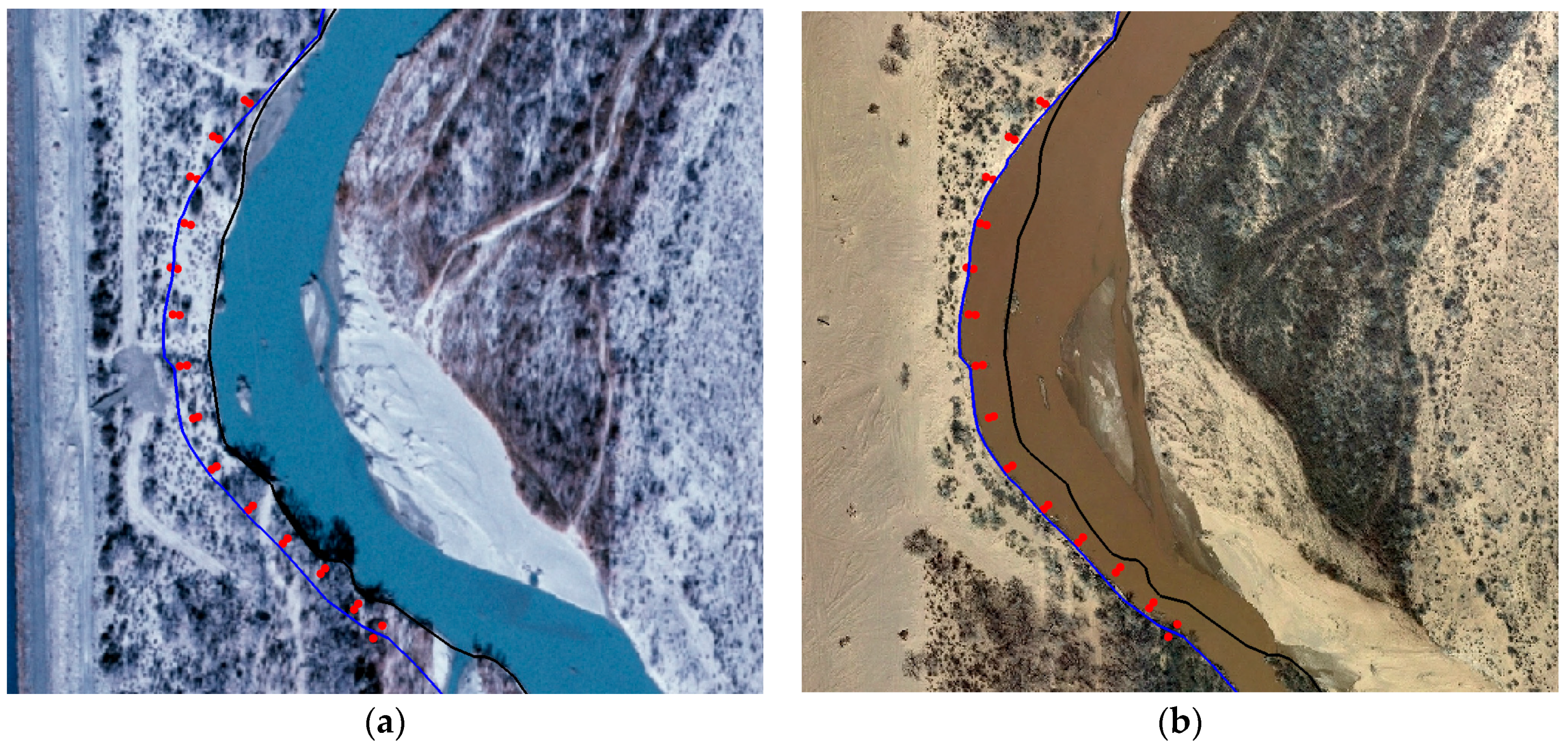
The combined vertical and lateral simulation is carried out next and results are presented. Among several model inputs, the erodibility coefficient is found to be the major calibration parameter for the simulation. The predicted 2010 bankline, shown as red dots in Figure 7 representing bank toe and top nodes, is compared with the data (blue solid line). In the figure, the January 2006 and summer 2010 historical aerial photographs are also displayed for comparison. It is seen that the calibrated model does a reasonably good job in capturing the bank retreat over the five-year simulation period. Up to 23.8 m of bank retreat distance is predicted at several banks and it is in agreement with the historical data.
It is noted that the calibrated erodibility coefficient varies along the outer bank with its value reduced towards the downstream. For example, the erodibility value is 2.0 × 10⁻⁵ for banks 2 to 10, 5.0 × 10⁻⁶ for banks 11 to 12, and 2.0 × 10⁻⁶ from banks 13 to 15. The reduction along banks 11–15 may be justified as the banks in this section were reinforced by the presence of bushes as shown in Figure 7a. The presence of bushes with roots deep in the bank was also confirmed during the field trip in February 2013 by the author.
The five-year modeling at this site shows that the present combined vertical and lateral model is applicable to practical streams. The model is robust and simple to apply for engineering applications. The moving mesh approach works well for the case and the model results compare well with the available data. Despite the success, the simulation reveals also areas that need future attention. First, field investigation is recommended for the bank erosion site so that the dominant bank erosion mechanisms may be identified. The present model is valid primarily for fluvial processes. If non-fluvial processes are present, the model would be less accurate, although the erodibility coefficient may be adjusted to take those effects into account to a certain extent. In addition, the terrain data in the main channel of the retreating banks are too scarce (Figure 3a). The October 2005 terrain reconstructed from the cross section data is probably inaccurate. High uncertainty in terrain may cast doubts on the reasonableness of the calibrated erodibility coefficient. Erodibility coefficient is a physical parameter; however, it is possible that the calibrated value can contain non-physical components contributed by the terrain data uncertainty. A new bathymetric survey, with denser and more accurate measuring equipment, is recommended.
3.2. Bank Retreat: The Choshui River
The present model is next applied to simulate the vertical and lateral morphological processes of a Chosui River reach in Taiwan. Choshui River is the longest river in Taiwan with about 187 km in length, draining from an area of 3157 square kilometers watershed. Details about the river hydrology and geomorphic features may be found in Lai et al. [15].
Following the modeling procedure described for the Rio Grande case, the model domain is selected first, as shown in Figure 8a. The study reach is about 16.7 km long and an average of 1.9 km in width. It is located near the river mouth with an average slope of 1:900. The upstream boundary is located 2.9 km upstream of the Ziqiang bridge and the downstream boundary is 1.8 km downstream of the Xibin bridge. The study reach is challenging to simulate as it is of the multi-channel braided type and subject to significant morphological changes. In addition, both moving mesh and fixed mesh approaches are used for the modeling to evaluate the pros and cons of each. With the model domain determined, a 2D mesh is generated consisting of 16,698 mixed quadrilateral and triangular mesh cells. This initial mesh is used by both the moving mesh and fixed mesh approaches.
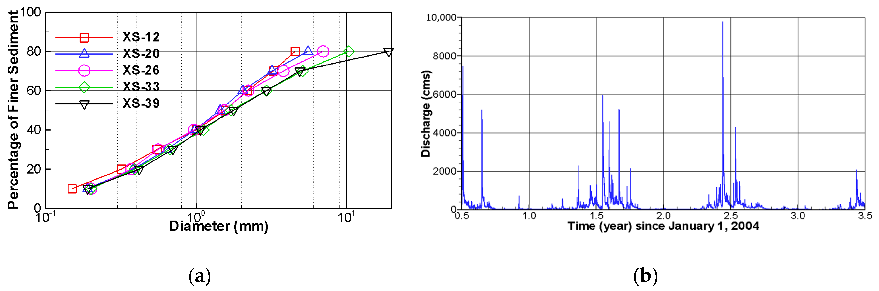
A three-year simulation is carried out from July 2004 to August 2007. The initial river bathymetry was based on the field measured bed elevation in April 2004 (black lines in Figure 8a) and the final bathymetry used by the model is shown in Figure 8b. Interpolation from the field data to the model is performed with the SMS software. The key model inputs are as follows. The flow resistance is represented by the Manning’s coefficient (n) and a constant value of n = 0.027, estimated using the field data, is adopted. The initial bed gradation is based on the measurement carried out in April 2004. The data showed that the bed had a medium diameter of 1.44~1.78 mm during the simulation period. Five data points within the study area are plotted in Figure 9a. Five sediment size classes are used to represent the range of sediments in the river: (1) 0.0625–0.125 mm; (2) 0.125–0.25 mm; (3) 0.25–0.5 mm; (4) 0.5–2.0 mm; and (5) 2.0–32 mm. The Engelund–Hansen sediment capacity equation [34] is used to compute the erosional rate potential as this equation is suitable for sandy rivers. At the upstream boundary, the hourly recorded discharge data are used as the boundary condition (Figure 9b) while the sediment supply rate is estimated to be 75% of the capacity computed by the Engelund–Hansen equation. At the downstream boundary, the stage-discharge rating curve developed from the measured data is used.
Model inputs specific to the lateral bank erosion model are presented next. A section of the left bank is selected for bank retreat modeling along with vertical processes in the channels. The bank zone, represented by the 2D mesh, is shown in Figure 10 in which bank toe and top bank lines are also marked. A total of 21 banks, shown as black circles, are used for bank retreat modeling. The bank erosion parameters are as follows: (a) a constant time step of one hour is used with the bank module (the time step for the vertical model is 5 s); and (b) all banks have a porosity of 0.3 (measured), the critical shear stress of 0.5 Pa (estimated from field data), erodibility of 3.0 × 10⁻⁵ (calibrated), the angle of repose of 30° (estimated), and the volumetric sediment composition of 0.5, 0.35, 0.15, 0.0, and 0.0 for the five size classes (measured), respectively. The critical shear stress of 0.5 Pa is estimated based on the 0.045 critical Shields parameter and 0.65 mm diameter. Again, this modeling shows that the erodibility coefficient is the only major parameter that should be calibrated using the measured bank retreat data. For the present simulation, the same erodibility is used for all banks as the bank properties do not vary much from each other based on field observations. During the continuous dynamic simulation, the materials eroded from the bank is deposited to the nearby channels.
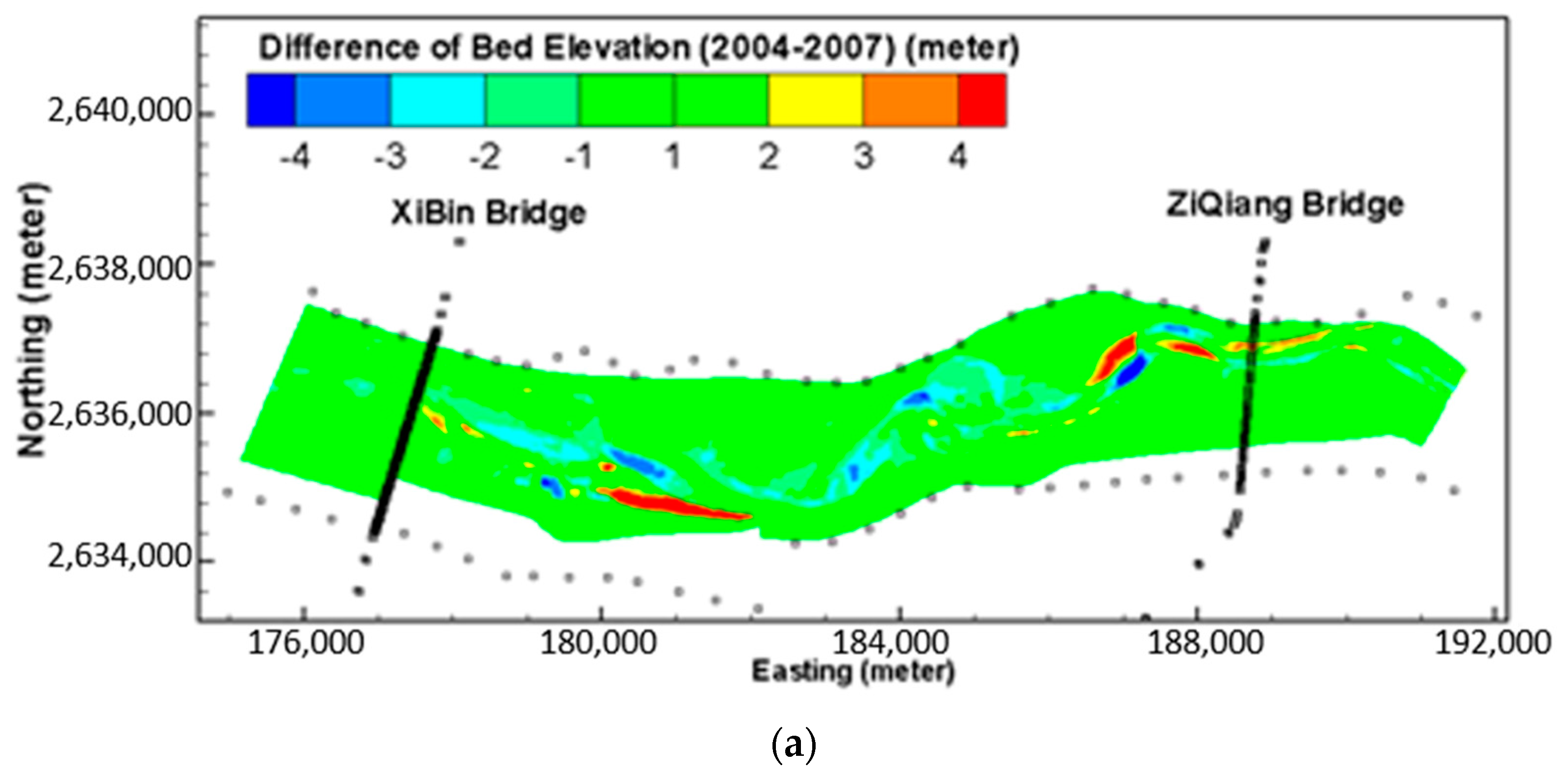
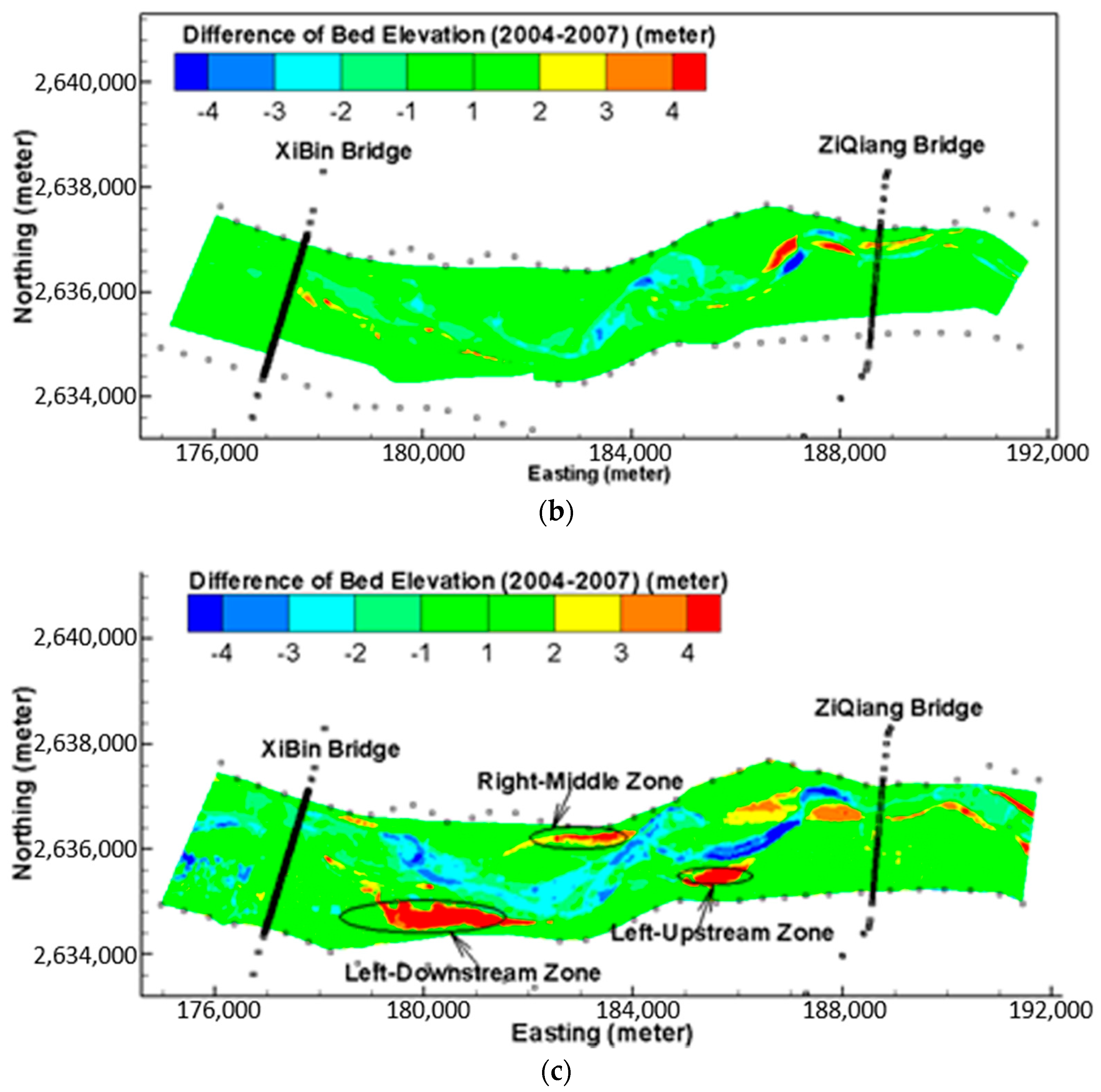
The combined vertical and lateral simulation is carried out from July 2004 to August 2007 (3-year) using both the moving mesh and fixed mesh approaches. A comparison of the predicted and measured net erosion and deposition depth over the three-year period is shown in Figure 11 for both mesh approaches. Large mismatch is observed upstream of the Ziqiang bridge near the upstream boundary. It is expected as the upstream boundary is located within a bend and results near the boundary are less accurate. Immediately downstream of the Ziqiang bridge, the model correctly predicts the “straightening” trend of the channel. Both immediate bars downstream of the bridge are eroded but the corresponding opposite banks of the bars experience aggradation. The model predicts the observed erosion trend in the area marked as “Left_Upstream Zone” in Figure 11c. The predicted erosion depth, however, is much less than the measured data and the extent is also not well predicted. The mismatch may be attributed to unaccounted flows: the area was impacted by the tributary flow nearby which is not incorporated by the numerical model due to lack of data. Bank erosion marked as “Right-Middle Zone” is not predicted by the model at all. Attempts have been made to simulate this zone by activating the lateral model along the banks. Such efforts are unsuccessful as it is found that there is very few water actually flowing towards this area. It is conjectured that the bank erosion in this zone is due probably to undocumented events. Possible causes include: (a) local peculiar topographic features that caused water directed towards the area but not captured by the model; (b) impact of the tributary flow on the opposite side of the bank which is not included by the model; and (c) bank failure due to non-fluvial processes. The bank marked as “Left-Downstream Zone” has experienced large and rapid bank retreat during the simulation period. Both moving and fixed mesh approaches encounter problems. Both models predict reasonable bank erosion but retreat distance is under-predicted. With the moving mesh approach, further increase of the erodibility coefficient to match the measured bank retreat distance is not possible; the model would diverge as the mesh representing the eroding bank has been distorted too much. With the fixed mesh approach, the simulated bank retreat distance is highly dependent on the mesh density. With the current mesh used, it is insufficient to represent each bank well leading to gross under-prediction of the bank erosion. The needed increase in mesh density results in prohibitively long computing time and it is abandoned during the study. Overall, the model predicts the overall erosion and deposition patterns, but the agreement is more qualitative than quantitative.
This application case demonstrates that the present vertical and lateral model can predict the gross erosion and deposition patterns and bank erosion processes although the river is subject to rapid and significant bank retreat. Agreement with the measured data is good quantitatively in some areas but only qualitatively in others. The uncertainty in bed gradation spatial distribution and lack of such data are partially responsible for the less satisfactory model predictions. In the current study, the bed gradation survey was carried out mostly at exposed bars which tend to underestimate the sediment size in the main channel. The modeling shows that even current state-of-the-art models are not yet able to make a quantitative prediction of bank erosions for braided or morphologically dynamic river systems such as the Chosui River. For such complex rivers, accurate measured data of bed gradation distribution is important. Without such data, the model may only be used for qualitative prediction of the future morphological trend and identification of potential erosion and deposition trouble spots.
4. Summary and Future Needs
An extended vertical and lateral bank erosion model is developed. A fixed mesh approach is proposed and implemented in addition to the moving mesh approach. Two practical streams with significant bank erosions are simulated to demonstrate the performance of the model, establish the modeling procedure, identify key model inputs, and reveal model limitations.
The study shows that the bank erosion model is robust and ready to use for engineering applications. Comparisons of the model results with the available data show that the model is only quantitative in some variables or areas and qualitative in others. For example, the model may predict the bank retreat distance over a specified period reasonably well but the overall erosion and deposition patterns only qualitatively.
This study has established the modeling procedure, as defined in the Rio Grande simulation case. It is simple to follow and no more complex than non-bank erosion modeling. Despite many model inputs needed, the study find that two model inputs are the most important for vertical erosion processes: the flow roughness coefficient and the initial bed gradation. For lateral bank erosion modeling, the most important calibration parameter is the erodibility coefficient that quantifies the rate of retreat at each simulated bank. The erodibility coefficient adopted in the model represents primarily fluvial processes. It, however, may be used to include other contributions such as the reinforcements by vegetation roots or bank protection materials. The erodibility coefficient may even be used to represent non-fluvial processes if they can be identified and quantified in the field. Once calibrated, the numerical model can perform a reasonable job in predicting bank retreat distance. Considering that the measured bank erodibility may vary by an order of magnitude, it is recommended that the erodibility parameter is treated as a calibration parameter.
Despite success achieved, the study reveals also areas that need future attention for model improvements. First, the mechanistic failure bank erosion model of Lai et al. [22] is found to be potentially unstable for practical stream modeling though it worked well for less complex cases. The uniform retreat model is found to be much more robust and can produce stable predictions. In the future, research is needed to understand how the erodibility coefficient of the uniform retreat model may be parameterized to the root strength and density so that the vegetation effects on bank erosion may be simulated. Second, the study finds that the moving mesh approach is more accurate and requires much less mesh points than the fixed mesh approach. It, however, works well only for small to moderate retreat distance (less than one stream width). The model may fail for banks experiencing large erosion (e.g., more than one stream width) due to excessive mesh distortions. The fixed mesh approach, on the other hand, is robust in that it does not suffer from the mesh-distortion related instability. It, however, requires a much refined mesh to represent the bank accurately. It is found that the model results using the fixed mesh are much less accurate than those of the moving mesh unless significantly more mesh points are used. High-resolution mesh modeling for practical streams can be prohibitive given the usual computational power currently available for engineers is desktop PCs. In the future, a hybrid approach may be developed so that vertical and lateral predictions are based on the moving mesh but a locally adaptive and fixed mesh is used to store model results.
Conflicts of Interest
The author declares no conflict of interest.
References
- Environment Agency. Waterway Bank Protection: A Guide to Erosion Assessment and Management; R and D Publication 11; Environment Agency: Bristol, UK, 1999; 235p.
- Florsheim, J.L.; Mount, J.F.; Chin, A. Bank erosion as a desirable attribute of rivers. Bioscience 2008, 58, 519–529. [Google Scholar] [CrossRef]
- Van der Mark, C.F.; van der Sligte, R.A.M.; Becker, A.; Mosselman, E.; Verheij, H.J. A method for systematic assessment of the morphodynamic response to removal of bank protection. River Flow 2012. In Proceedings of the International Conference on Fluvial Hydraulics, San Jose, Costa Rica, 5–7 September 2012. [Google Scholar]
- Juez, C.; Bühlmann, I.; Maechler, G.; Schleiss, A.J.; Franca, M.J. Transport of suspended sediments under the influence of bank macro-roughness. Earth Surf. Process. Landf. 2017. [Google Scholar] [CrossRef]
- Lai, Y.G. Erosion Analysis Upstream of the San Acacia Diversion Dam on the Rio Grande; Technical Report; Technical Service Center, Bureau of Reclamation: Denver, CO, USA, 2007.
- Lai, Y.G.; Greimann, B.P. Predicting contraction scour with a two-dimensional depth-averaged model. J. Hydraul. Res. 2010, 48, 383–387. [Google Scholar] [CrossRef]
- Lai, Y.G.; Greimann, B.P.; Wu, K. Soft bedrock erosion modeling with a two-dimensional depth-averaged model. J. Hydraul. Eng. 2011, 137, 804–814. [Google Scholar] [CrossRef]
- Juez, C.; Murillo, J.; García-Navarro, P. A 2D weakly-coupled and efficient numerical model for transient shallow flow and movable bed. Adv. Water Resour. 2014, 71, 93–109. [Google Scholar] [CrossRef]
- Chen, D.; Duan, J.G. Modeling width adjustment in meandering channels. J. Hydrol. 2006, 321, 59–76. [Google Scholar] [CrossRef]
- ASCE Task Committee on Hydraulics; Bank Mechanics and Modeling of River Width Adjustment. River width adjustment, II: Modeling. J. Hydraul. Eng. 1998, 124, 903–917. [Google Scholar]
- Rinaldi, M.; Darby, S.E. Modelling river-bank-erosion processes and mass failure mechanisms: Progress towards fully coupled simulations. In Gravel-Bed Rivers 6: From Process Understanding to River Restoration; Developments in Earth Surface Processes 11; Habersack, H., Piégay, H., Rinaldi, M., Eds.; Elsevier: Amsterdam, The Netherlands, 2008; pp. 213–239. [Google Scholar]
- Langendoen, E.J.; Simon, A. Modeling the evolution of incised streams. II: Streambank erosion. J. Hydraul. Eng. 2008, 134, 905–915. [Google Scholar] [CrossRef]
- Motta, D.; Abad, J.D.; Langendoen, E.J.; Garcia, M.H. A simplified 2D model for meander migration with physically-based bank evolution. Geomorphology 2012, 163–164, 10–25. [Google Scholar] [CrossRef]
- Lai, Y.G. Advances in geofluvial modeling: Methodologies and applications. In Advances in Water Resources Engineering, Handbook of Environmental Engineering; Yang, C.T., Wang, L.K., Eds.; Humana Press: New York, NY, USA; Springer Science and Business Media: Cham, Switzerland, 2014; Volume 14. [Google Scholar]
- Lai, Y.G. A Coupled Stream Bank Erosion and Two-Dimensional Mobile-Bed Model; Technical Report, SRH-2013-07; Technical Service Center, Bureau of Reclamation: Denver, CO, USA, 2013.
- Mosselman, E. Mathematical modeling of morphological processes in rivers with erodible cohesive banks. In Communications on Hydraulic and Geotechnical Engineering; Delft University of Technology: Delft, The Netherlands, 1998; Volume 92. [Google Scholar]
- Darby, S.E.; Alabyan, A.M.; van de Wiel, M.J. Numerical simulation of bank erosion and channel migration in meandering rivers. Water Resour. Res. 2002, 38, 1163–1183. [Google Scholar] [CrossRef]
- Nagata, N.; Hosoda, T.; Muramoto, Y. Numerical analysis of river channel processes with bank erosion. J. Hydraul. Eng. 2000, 126, 243–252. [Google Scholar] [CrossRef]
- Duan, G.; Wang, S.S.Y.; Jia, Y. The applications of the enhanced CCHE2D model to study the alluvial channel migration processes. J. Hydraul. Res. 2001, 39, 469–480. [Google Scholar] [CrossRef]
- Langendoen, E.J. CONCEPTS—Conservational Channel Evolution and Pollutant Transport System; Research Report No. 16; USDA, Agricultural Research Service, National Sedimentation Laboratory: Oxford, MS, USA, 2000.
- Simon, A.; Curini, A.; Darby, S.E.; Langendoen, E.J. Bank and near-bank processes in an incised channel. Geomorphology 2000, 35, 193–217. [Google Scholar] [CrossRef]
- Lai, Y.G.; Thomas, R.; Ozeren, Y.; Simon, A.; Greimann, B.P.; Wu, K. Modeling of multi-layer cohesive bank erosion with a coupled bank stability and mobile-bed model. Geomorphology 2015, 243, 116–129. [Google Scholar] [CrossRef]
- Simon, A.; Pollen-Bankhead, N.; Thomas, R.E. Development and application of a deterministic bank stability and toe erosion model for stream restoration. In Stream Restoration in Dynamic Fluvial Systems: Scientific Approaches, Analyses and Tools; Geophysical Monograph Series 194; American Geophysical Union: Washington, DC, USA, 2011; pp. 453–474. [Google Scholar]
- Lai, Y.G. Two-dimensional depth-averaged flow modeling with an unstructured hybrid mesh. J. Hydraul. Eng. 2010, 136, 12–23. [Google Scholar] [CrossRef]
- Lai, Y.G. SRH-2D Theory and User’s Manual Version 2.0; Technical Service Center, Bureau of Reclamation: Denver, CO, USA, 2008.
- Lai, Y.G.; Weber, L.J.; Patel, V.C. Non-hydrostatic three-dimensional method for hydraulic flow simulation—Part I: Formulation and verification. J. Hydraul. Eng. 2003, 129, 196–205. [Google Scholar] [CrossRef]
- Greimann, B.P.; Lai, Y.G.; Huang, J. Two-dimensional total sediment load model equations. J. Hydraul. Eng. 2008, 134, 1142–1146. [Google Scholar] [CrossRef]
- Hasegawa, K. Bank-erosion discharge based on a nonequilibrium theory. JSCE 1981, 316, 37–50. (In Japanese) [Google Scholar]
- Osman, M.A.; Thorne, C.R. Riverbank stability analysis: I. Theory. J. Hydraul. Eng. 1988, 114, 134–150. [Google Scholar] [CrossRef]
- Bauer, T.R. Bed Material Sampling on the Middle Rio Grande, New Mexcico; U.S. Bureau of Reclamation, Technical Service Center, Sedimentation and River Hydraulics Group: Denver, CO, USA, 2006.
- Parker, G. Surface-based bedload transport relation for Gravel Rivers. J. Hydraul. Res. 1990, 28, 417–436. [Google Scholar] [CrossRef]
- Lai, Y.G. Sediment Plug Prediction on the Rio Grande with SRH-2D Model; Technical Report, SRH-2009-41; Technical Service Center, U.S. Bureau of Reclamation: Denver, CO, USA, 2009.
- Lai, Y.G. Prediction of Channel Morphology Upstream of Elephant Butte Reservoir on the Middle Rio Grande; Technical Report, SRH-2011-04; Technical Service Center, U.S. Bureau of Reclamation: Denver, CO, USA, 2011.
- Engelund, F.; Hansen, E. A Monograph on Sediment Transport in Alluvial Streams; Teknish Forlag, Technical Press: Copenhagen, Denmark, 1972. [Google Scholar]
Figure 1.
Diagram of bank retreat computation with the uniform retreat model (red line G’ABC is the initial bank; green line GFIBC is the bank profile after basal erosion; and blue line GDIE is the final bank profile after bank failure).
Figure 1.
Diagram of bank retreat computation with the uniform retreat model (red line G’ABC is the initial bank; green line GFIBC is the bank profile after basal erosion; and blue line GDIE is the final bank profile after bank failure).

Figure 2.
Illustration of a channel reach for the modeling with right bank being eroded (blue area is bank zone 1; green area is bank zone 2; red-cross zone is the stream main channel).
Figure 2.
Illustration of a channel reach for the modeling with right bank being eroded (blue area is bank zone 1; green area is bank zone 2; red-cross zone is the stream main channel).

Figure 3.
Solution domain (a); 2D mesh (b); and terrain (c) for the study site of middle Rio Grande (blue lines in (a) represent the locations for the bathymetry survey data).
Figure 3.
Solution domain (a); 2D mesh (b); and terrain (c) for the study site of middle Rio Grande (blue lines in (a) represent the locations for the bathymetry survey data).
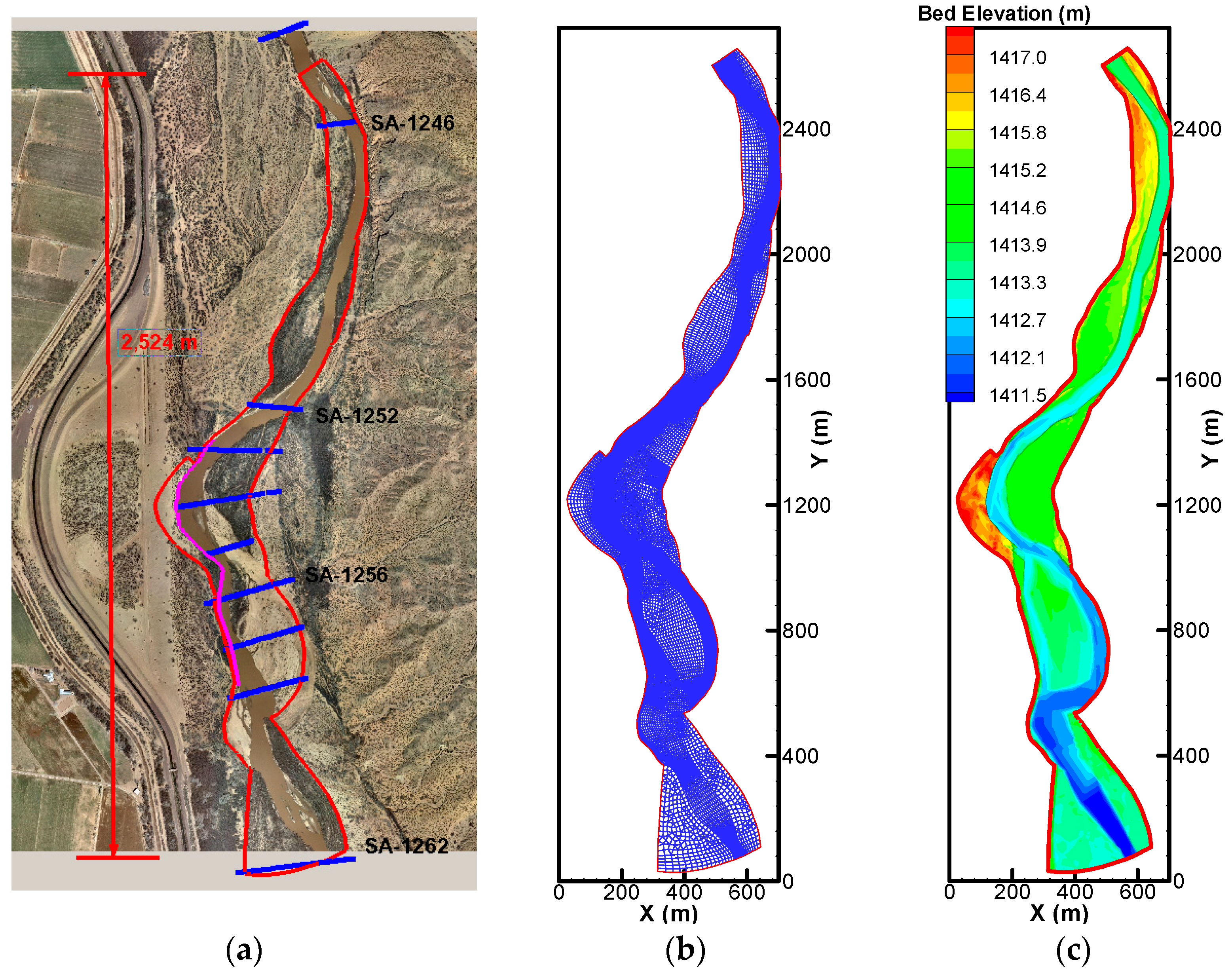
Figure 4.
Thirteen [13] survey locations for bed gradation along with the measured cumulative distribution of bed sediments at all survey points (Points 50 #1 and #2, Points 52 #1 and #2 and Points 54 #1 and #2 are close but not at the same locations): (a) Survey Points; (b) Points 51–54 and 56; and (c) Points 50, 54, 56.
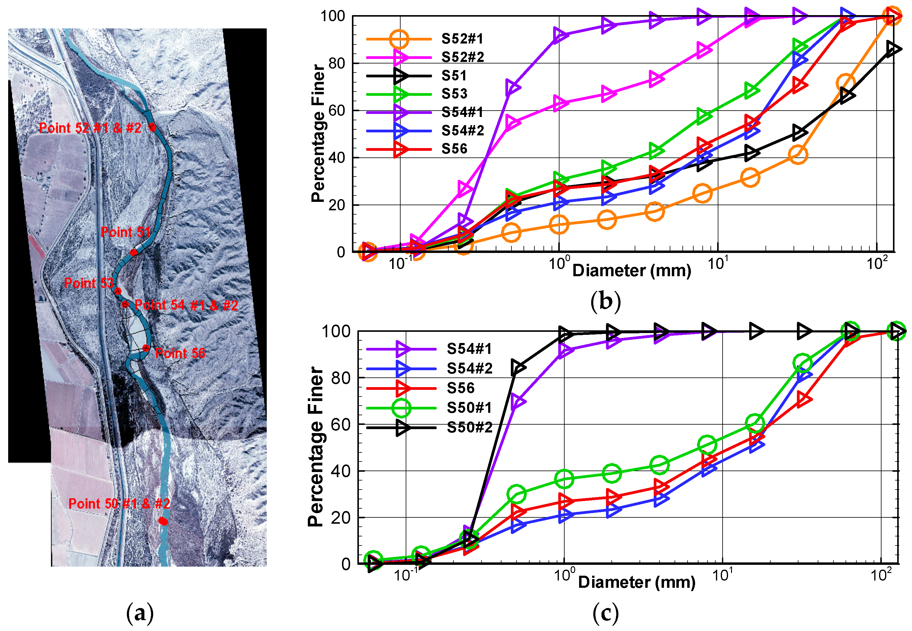
Figure 5.
Daily flow discharge data (left) and the bank zone used for the simulation (red dots represent bank toe nodes and black dots are bank top nodes): (a) discharge hydrograph; and (b) bank zone.
Figure 5.
Daily flow discharge data (left) and the bank zone used for the simulation (red dots represent bank toe nodes and black dots are bank top nodes): (a) discharge hydrograph; and (b) bank zone.
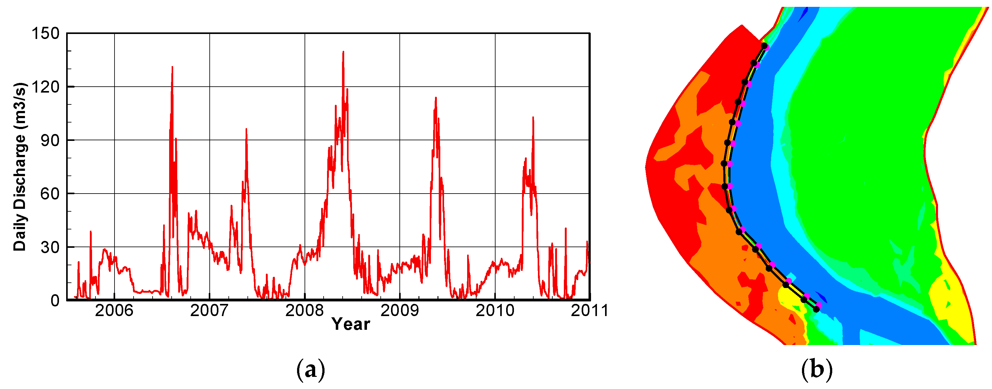
Figure 6.
Simulated velocity and shear stress distributions at 28.32 m3/s discharge for the Rio Grande case: (a) velocity overview; (b) velocity close-up view; and (c) shear stress close-up view.
Figure 6.
Simulated velocity and shear stress distributions at 28.32 m3/s discharge for the Rio Grande case: (a) velocity overview; (b) velocity close-up view; and (c) shear stress close-up view.
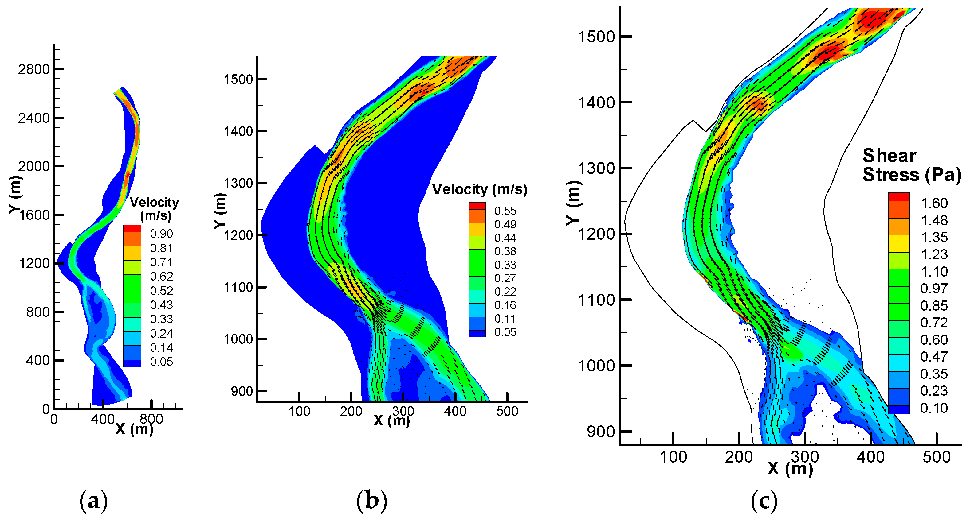
Figure 7.
Comparison of the predicted bankline and the historical bankline changes (black line: January 2006 line; blue line: summer 2010 line; red dots: Predicted 2010 line): (a) January 2006 serial photo; and (b) Summer 2010 aerial photo.
Figure 7.
Comparison of the predicted bankline and the historical bankline changes (black line: January 2006 line; blue line: summer 2010 line; red dots: Predicted 2010 line): (a) January 2006 serial photo; and (b) Summer 2010 aerial photo.

Figure 8.
Model domain selected for the Chosui River modeling (aerial photo is in August 2007) and the bed elevation reconstructed from the survey data in April 2004: (a) model domain (black lines are survey sections); and (b) terrain.
Figure 8.
Model domain selected for the Chosui River modeling (aerial photo is in August 2007) and the bed elevation reconstructed from the survey data in April 2004: (a) model domain (black lines are survey sections); and (b) terrain.
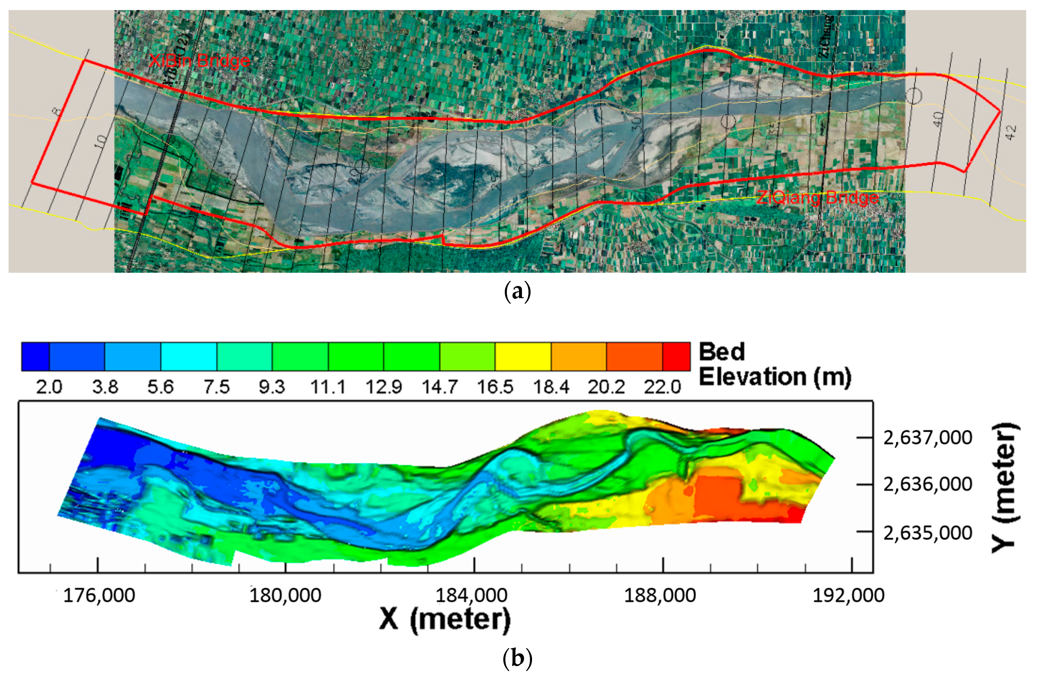
Figure 9.
Initial bed gradation in 2004 (a) and flow hydrograph from July 2004 to August 2007 (b).

Figure 10.
The bank zone (black polygon) represented by the 2D mesh. Top black filled dots represent bank toes of all banks and lower dots are bank top nodes.
Figure 10.
The bank zone (black polygon) represented by the 2D mesh. Top black filled dots represent bank toes of all banks and lower dots are bank top nodes.
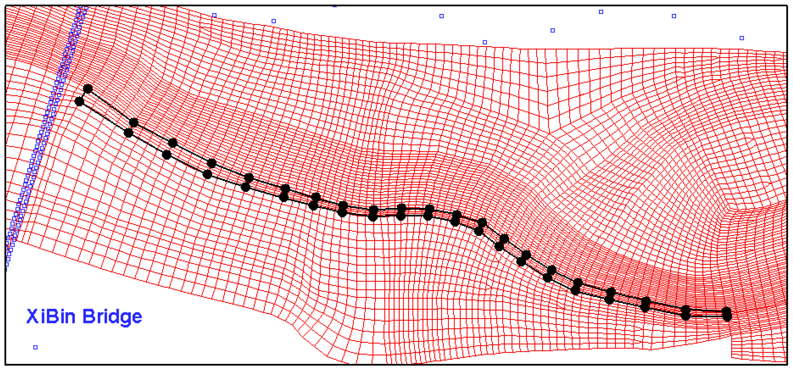
Figure 11.
Predicted and measured net erosion (positive) and deposition (negative) depth from July 2004 to August 2007 for the Choshui River case: (a) prediction with moving mesh; (b) prediction with fixed mesh; and (c) measured data.
Figure 11.
Predicted and measured net erosion (positive) and deposition (negative) depth from July 2004 to August 2007 for the Choshui River case: (a) prediction with moving mesh; (b) prediction with fixed mesh; and (c) measured data.


Table 1.
Size ranges of seven sediment size classes used for the Rio Grande modeling.
| Sediment Size Class | Size Range (mm) |
|---|---|
| 1 | 0.002 to 0.0625 |
| 2 | 0.0625 to 0.25 |
| 3 | 0.25 to 0.5 |
| 4 | 0.5 to 2.0 |
| 5 | 2.0 to 8.0 |
| 6 | 8.0 to 32 |
| 7 | 32 to 125 |
© 2017 by the author. Licensee MDPI, Basel, Switzerland. This article is an open access article distributed under the terms and conditions of the Creative Commons Attribution (CC BY) license (http://creativecommons.org/licenses/by/4.0/).
Share and Cite
MDPI and ACS Style
Lai, Y.G. Modeling Stream Bank Erosion: Practical Stream Results and Future Needs. Water 2017, 9, 950. https://doi.org/10.3390/w9120950
AMA Style
Lai YG. Modeling Stream Bank Erosion: Practical Stream Results and Future Needs. Water. 2017; 9(12):950. https://doi.org/10.3390/w9120950
Chicago/Turabian StyleLai, Yong G. 2017. "Modeling Stream Bank Erosion: Practical Stream Results and Future Needs" Water 9, no. 12: 950. https://doi.org/10.3390/w9120950
Note that from the first issue of 2016, this journal uses article numbers instead of page numbers. See further details here.