Transient Modeling of Flow in Unsaturated Soils Using a Novel Collocation Meshless Method


Department of Harbor and River Engineering, National Taiwan Ocean University, Keelung 20224, Taiwan
*
Author to whom correspondence should be addressed.
Water 2017, 9(12), 954; https://doi.org/10.3390/w9120954
Submission received: 1 November 2017
/
Revised: 1 December 2017
/
Accepted: 4 December 2017
/
Published: 7 December 2017
(This article belongs to the Special Issue Soil Water Conservation: Dynamics and Impact)
Abstract
:In this paper, a novel meshless method for the transient modeling of subsurface flow in unsaturated soils was developed. A linearization process for the nonlinear Richards equation using the Gardner exponential model to analyze the transient flow in the unsaturated zone was adopted. For the transient modeling, we proposed a pioneering work using the collocation Trefftz method and utilized the coordinate system in Minkowski spacetime instead of that in the original Euclidean space. The initial value problem for transient modeling of subsurface flow in unsaturated soils can then be transformed into the inverse boundary value problem. A numerical solution obtained in the spacetime coordinate system was approximated by superpositioning Trefftz basis functions satisfying the governing equation for boundary collocation points on partial problem domain boundary in the spacetime coordinate system. As a result, the transient problems can be solved without using the traditional time-marching scheme. The validity of the proposed method is established for several test problems. Numerical results demonstrate that the proposed method is highly accurate and computationally efficient. The results also reveal that it has great numerical stability for the transient modeling of subsurface flow in unsaturated soils.
1. Introduction
Increasing interest has been shown in recent years in understanding the behavior of unsaturated soils. The prediction of moisture flow under transient conditions is important in engineering practice when considering such practical problems as the design of shallow foundations, pavements, and the stability of unsaturated soil slopes [1,2,3,4]. As a result, unsaturated flow has become one of the most important and active topics of research. A complete theory of subsurface flow when rainfall infiltrates unsaturated zones can be described using either the variably saturated flow equation or the generalized Richards equation [5]. The Richards equation is a highly nonlinear equation governed by nonlinear physical relationships. Nonlinear physical relationships can be described using soil–water characteristic curves [6,7,8]. Since the Richards equation is highly nonlinear and cannot directly provide an analytical solution, modeling flow process in unsaturated soils is usually based on the numerical solutions of the Richards equation [9,10,11,12,13,14,15].
Numerical approaches to the simulation of the Richards equation using the mesh-based methods, such as the finite difference method [16,17,18,19] or the finite element method [20,21,22,23], are well documented in the past. Despite the great success of the mesh-based methods as effective numerical tools for the solution of problems on complex domains, there is still growing interest in the development of new advanced computational methods [24,25,26]. Meshless methods emerge as a competitive alternative to discretization methods. Differing from conventional mesh-based methods, the meshless method has the advantages that it does not need the mesh generation [27]. Problems involving regions of irregular geometry are generally intractable analytically [28]. For such problems, the use of numerical methods, especially the boundary-type meshless method, to obtain approximate solutions is advantageous [29]. A significant number of such methods have been proposed, such as the Trefftz method [30,31], the method of fundamental solution [32,33], the element-free Galerkin method [34], the reproducing kernel particle method [35], and the meshless local Petrov–Galerkin approach [36].
The Trefftz method is probably one of the most popular boundary-type meshless methods for solving boundary value problems where approximate solutions are expressed as a linear combination of functions automatically satisfying governing equations [37,38]. Li et al. [39] provided a comprehensive comparison of the Trefftz method, collocation, and other boundary methods, concluding that the collocation Trefftz method (CTM) is the simplest algorithm and provides the most accurate solutions with optimal numerical stability. Because the Trefftz method is originally developed to deal with the boundary value problems in Euclidean space, the application the Trefftz method for solving time-dependent problems is hardly found.
In this paper, we proposed a pioneering work using the CTM for transient modeling of subsurface flow in unsaturated soils. Since the Richards equation is highly nonlinear, we first proposed a linearization process for the nonlinear Richards equation using the Gardner exponential model [40,41]. To deal with the transient modeling, we adopted the coordinate system in Minkowski spacetime instead of that in the original Euclidean space [42,43]. Based on Minkowski spacetime, we assume that time is an absolute physical quantity that plays the role of the independent variable such that the spacetime coordinate system is a mathematically (n + 1)-dimensional system including n-dimensional space and one-dimensional of time [44]. In the spacetime coordinate system, both the initial and boundary conditions can be treated as boundary conditions on the spacetime domain boundary. Since the solution of final time on the other boundary of the domain is unknown, it becomes an inverse boundary value problem which is to seek an unknown boundary function on boundaries inaccessible for data measurement with the over specified boundary data on boundaries accessible for data measurement. The initial value problem for transient modeling of subsurface flow in unsaturated soils can then be transformed into the inverse boundary value problem.
A numerical solution obtained in the spacetime coordinate system was approximated by superpositioning Trefftz basis functions satisfying the governing equation for boundary collocation points on partial domain boundary in the spacetime coordinate system. As a result, the transient problems can be solved without using the traditional time-marching scheme. The validity of the proposed method is established for several test problems, including the investigation of the accuracy and the comparison of the numerical with analytical solutions. Application examples of the steady-state, the one-dimensional and two-dimensional transient problems of subsurface flow in unsaturated soils were carried out.
2. Trefftz Method for Modeling Subsurface Flow in Unsaturated Soils
2.1. The Linearized Richards Equation
For modeling subsurface flow in unsaturated soil, the Richards equation is commonly used and it may be written in three different forms such as the -based form, the -based form, and the mixed form. In this study, the -based form is adopted. A complete three-dimensional Richards equation [5] can be expressed as
where is the pressure head, is time, points down the ground surface, points to the tangent of the topographic contour passing through the origin, is the vertical coordinate, normal to the plane, , , and are the unsaturated hydraulic conductivity functions in lateral directions and the vertical direction, respectively, and is the specific moisture capacity function defined by
where is the moisture content. The Richards equation, as shown in Equation (1), is highly nonlinear because , , and are functions of . To solve the Richards equation, three characteristic functions are required and they are the unsaturated hydraulic conductivity function, the soil–water characteristic curve, and the specific moisture capacity function [19]. Assuming that the unsaturated soils are homogeneous and isotropic, the Richards equation governing two-dimensional flow in unsaturated soils can be obtained as
It is common to normalize the hydraulic conductivity of unsaturated soil with respect to their maximum value. The normalized value can be expressed as
where is the saturated hydraulic conductivity, and is the relative hydraulic conductivity which is a function of the pressure head. The governing equation can be obtained by substituting Equation (4) into Equation (3),
The above equation is the two-dimensional Richards equation. Gardner (1958) [40] proposed a simple one-parameter exponential model as
where is the parameter which is related to the pore size distribution of soil, and is the effective saturation defined by normalizing volumetric water content with its saturated and residual values as
where represents the residual water content, and represents the saturated water content. Substituting Equation (7) into Equation (6), we have,
Using the Gardner exponential model, the linearized Richards equation for two-dimensional transient, two-dimensional steady-state and one-dimensional transient Richards equations can be derived [46] as follows, respectively.
where , is the pressure head of the linearized Richards equation which can be defined as , and is the pressure head when the soil is dry.
2.2. The Trefftz Method in Euclidean Space
The CTM begins with the consideration of T-complete functions. For indirect Trefftz formulation, the approximated solution at the boundary collocation point can be written as a linear combination of the basis functions [31,47]. For a simply connected domain, one usually locates the source point inside the domain and the number of source point is only one for in the CTM [48,49].
Considering a two-dimensional domain, , in the polar coordinate, the Laplace governing equation can be written as
with
where and are the radius and polar angle in the polar coordinate system, denotes the outward normal direction, denotes the boundary where the Dirichlet boundary condition is given, denotes the boundary where the Neumann boundary condition is given, and denotes the Dirichlet boundary condition. For the Laplace equation, the particular solutions can be obtained using the method of the separation of variables. The particular solutions of Equation (13) include the following basis functions [50].
If we adopt the solution of a boundary value problem and enforce it to exactly satisfy the partial differential equation with the boundary conditions at a set of points, this leads to the CTM.
Considering a simply connected domain, the CTM for the Laplace equation can be expressed as
where , , and . m is the order of the T-complete basis functions for approximating the solution. , and are unknown coefficients to be determined. The accuracy of the solution for the CTM depends on the order of the basis functions. Usually, one may need to increase the m value to obtain better accuracy. However, the ill-posed behavior may also grow up with the increase of the m value [51].
2.3. The T Basis Function for Steady-State Linearized Richards Equation
For modeling subsurface flow in unsaturated soils using the CTM, we first started from the derivation of the CTM for the two-dimensional steady-state linearized Richards equation. The two-dimensional Richards governing equation can be expressed as Equation (5). Using the Gardner exponential model, the steady-state linearized Richards equation can be derived as
where is the steady-state pressure head of the linearized Richards equation. The standard process of the separation of variables can now be used by taking the steady-state solution as
Substituting Equation (19) into Equation (18) and dividing by gives
Each term in the above equation must be a constant for a nonzero solution, so the following are used.
where , is the positive integer, and is the characteristic length. It can be found that Equations (21) and (22) are simple ordinary differential equations that have solutions as
where , and and are arbitrary constants to be evaluated. If we considered a simply connected domain, the CTM for two-dimensional steady-state linearized Richards equation can be expressed as
where , , and . , , and are unknown coefficients determined by the collocation method. The basis for the T basis functions include four functions obtained from the separation of variables in the Cartesian coordinate system, which are listed in Table 1.
2.4. The Trefftz Method in Minkowski Spacetime
Considering a two-dimensional spacetime domain, , enclosed by a spacetime boundary, , the linearized Richards equation for two-dimensional transient subsurface flow in homogenous and isotropic confined porous medium can be expressed as
Considering the time dimension, the pressure head is the time-dependent variable. The initial condition can be described as
where denotes the distribution of the pressure head in the spacetime domain, , at time zero. To solve Equation (26), the boundary conditions must be given as follows.
where denotes the spacetime boundary where the Dirichlet boundary condition is given, denotes the spacetime boundary where the Neumann boundary condition is given, and denotes the Dirichlet boundary condition in the spacetime domain.
The transient pressure head of the linearized Richards equation [46,52] can be expressed as
where is the transient pressure head of the linearized Richards equation. The transient linearized Richards equation is determined by substituting Equation (30) into Equation (10), which gives
The standard process of the separation of variables may be used by having the transient solution as
Substituting Equation (32) into Equation (31) and dividing by gives
Each term in the above equation must be a constant for a nonzero solution, so the following are used.
where , is the positive integer, and is the characteristic length. The above equations are simple ordinary differential equations that have solutions,
where and are arbitrary constants to be evaluated. If we considered a simply connected domain, the CTM for two-dimensional transient linearized Richards equation can be expressed as
where , , and . , , and are unknown coefficients determined by the collocation method. m and o are the order of the T basis functions for approximating the solution. The basis for the T basis functions include four functions obtained from the separation of variables in the cartesian coordinate system, which are listed in Table 1.
Again, the CTM for one-dimensional transient linearized Richards equation can also be composed of a set of linearly independent vectors using the method of the separation of variables. Then, the solution can be derived as the linear combination of these basis functions.
where , , and . and are unknown coefficients determined by the collocation method. The basis for the T basis functions include three functions obtained from the separation of variables in the Cartesian coordinate system, which are listed in Table 2.
The above equations can be discretized at a number of collocated points on the spacetime boundary using the initial and boundary conditions. Then, we obtained a system of simultaneous linear equations as
where is a matrix with the size of aa × bb, with the size of bb × 1 is a vector of unknown coefficients, with the size of aa × 1 is a vector of function values at collocation points, aa is the number of collocation points, and bb is the number of the order of the T basis function. For simplicity, we adopted the commercial program MATLAB backslash operator to solve Equation (42).
3. Numerical Examples
3.1. Steady-State Modeling of Two-Dimensional Subsurface Flow in Unsaturated Soil
Meshless methods only rely on a series of random collocation points to discretize the spatial domain, which means not only onerous mesh generation is avoided, but also a more accurate description of irregular complex geometries can be achieved. Therefore, we investigated a two-dimensional steady-state unsaturated flow problem for an irregular boundary shape. With a two-dimensional simply connected domain, , enclosed by an irregular boundary, the governing equation is expressed as
A two-dimensional object boundary under consideration is defined as
where . The linearized governing equation is expressed as Equation (18). The boundary conditions are the Dirichlet boundary condition and the Dirichlet boundary data is applied using the following analytical solution.
Finally, the steady-state solution can be obtained using the following equation.
The soil is assumed to have the in the Gardner exponential model of . The pressure head when the soil is dry is assumed to be . The Dirichlet boundary condition is given on the boundaries using the analytical solution as shown in Equation (45). There are 51 boundary collocation points and a source point. We selected and , and adopted the commercial program MATLAB backslash operator to solve the system of simultaneous linear equations. Figure 1 depicts the computed pressure head distribution. Comparing with the analytical solution, it is found that highly accurate result in the order of can be obtained for this example, as depicted in Figure 2.
The previous example has demonstrated that the proposed method can be used to deal with the two-dimensional steady-state subsurface flow in unsaturated soils for an irregular boundary shape with very high accuracy. We further applied the proposed method to investigate the numerical solution of a two-dimensional steady-state Green–Ampt problem in the following section [53].
Figure 3 indicates a two-dimensional cross section of the soil with the dimensions of length and height , where a two-dimensional Green–Ampt problem is investigated. A pool of water at ground surface is maintained holding the pressure head. The specified pressure head, as shown in Equation (50), is applied at the top with pressure head set to zero in the center and tapering rapidly to dry conditions at two sides of the boundary, as shown in Figure 3. The parameter corresponding to the soil is also used. The bottom, left and right sides of the soil are in dry condition maintained as . Therefore, the boundary conditions can be expressed as
The analytical solution [46] of two-dimensional steady-state linearized Richards equation is given by
where and .
The steady-state solution can then be obtained using Equation (46). There are 200 boundary collocation points uniformly distributed in the boundary. We selected and for solving this example. The computed results are depicted in Figure 4 which demonstrates that the process of infiltration can continue if there is a pool of water at ground surface maintained holding the pressure head for additional water at the soil surface. It is found that the best accuracy of the proposed method can reach up to , as shown in Figure 5.
3.2. Transient Modeling of One-Dimensional Flow in Unsaturated Soil
The second example under investigation is the transient modeling of one-dimensional flow in unsaturated soil. The thickness of the soil (L) is 10 (m). The soil is assumed to have the in the Gardner exponential model of . The saturated hydraulic conductivity (), saturated water content (), and residual water content () of this example are (m/h), 0.35, and 0.14, respectively [54]. The total simulation time (T) is one hour (h). The governing equation can be expressed as follows.
Using the Gardner exponential model, the linearized governing equation can be expressed as Equation (12). The initial condition was the soil in dry condition maintained as . Thus,
The boundary conditions are the Dirichlet boundary condition. The Dirichlet boundary data are applied using the following analytical solution [46].
where . The can be obtained using the following equations.
Finally, the transient solution can be obtained as follows.
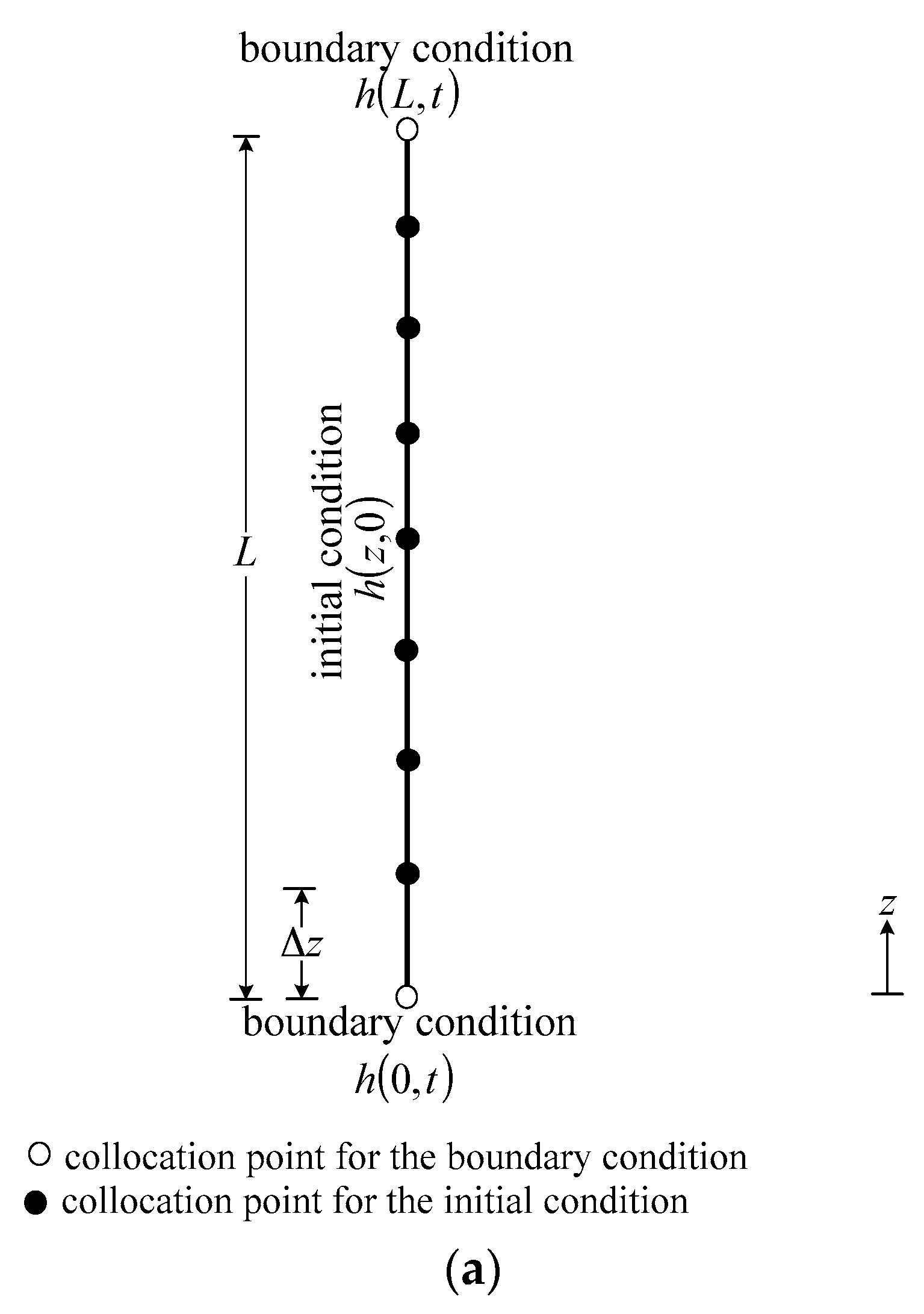
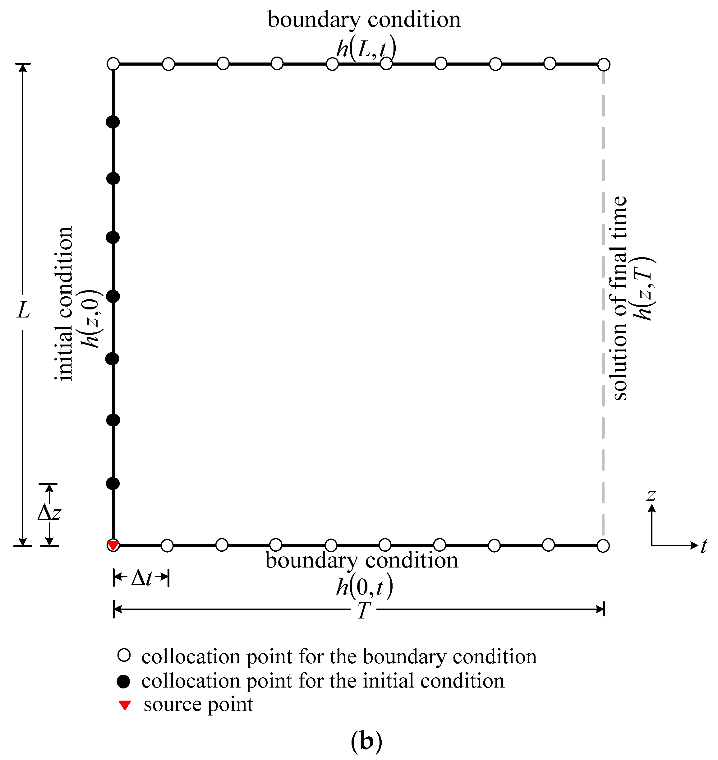
To deal with the transient modeling, we adopted the coordinate system in Minkowski spacetime instead of that in the original Euclidean space. Based on Minkowski spacetime, we assume that time is an absolute physical quantity that plays the role of the independent variable such that the spacetime coordinate system is a n-dimensional space and one-dimensional time. In this example, there is one-dimensional space and one-dimensional time. The spacetime domain is therefore a rectangular shape, as shown in Figure 6b. We transformed the one-dimensional initial value problem, as depicted in Figure 6a, for transient modeling of subsurface flow into two-dimensional inverse boundary value problem. It should be noted that the initial and boundary conditions are both applied on the spacetime boundary. In addition, it becomes an inverse boundary value problem because the right-side boundary values in Figure 6b were not assigned.
The initial condition was applied on the left side of the spacetime domain and the boundary conditions were applied on both top and bottom sides of the domain, as shown in Figure 6b. By selecting the space interval and time interval for 0.05 (m) and 0.05 (h), there are 375 boundary collocation points and a source point. The Dirichlet boundary values were given on boundary collocation points which collocated on three sides of the domain using the analytical solution for the problem. We selected and for solving this example.
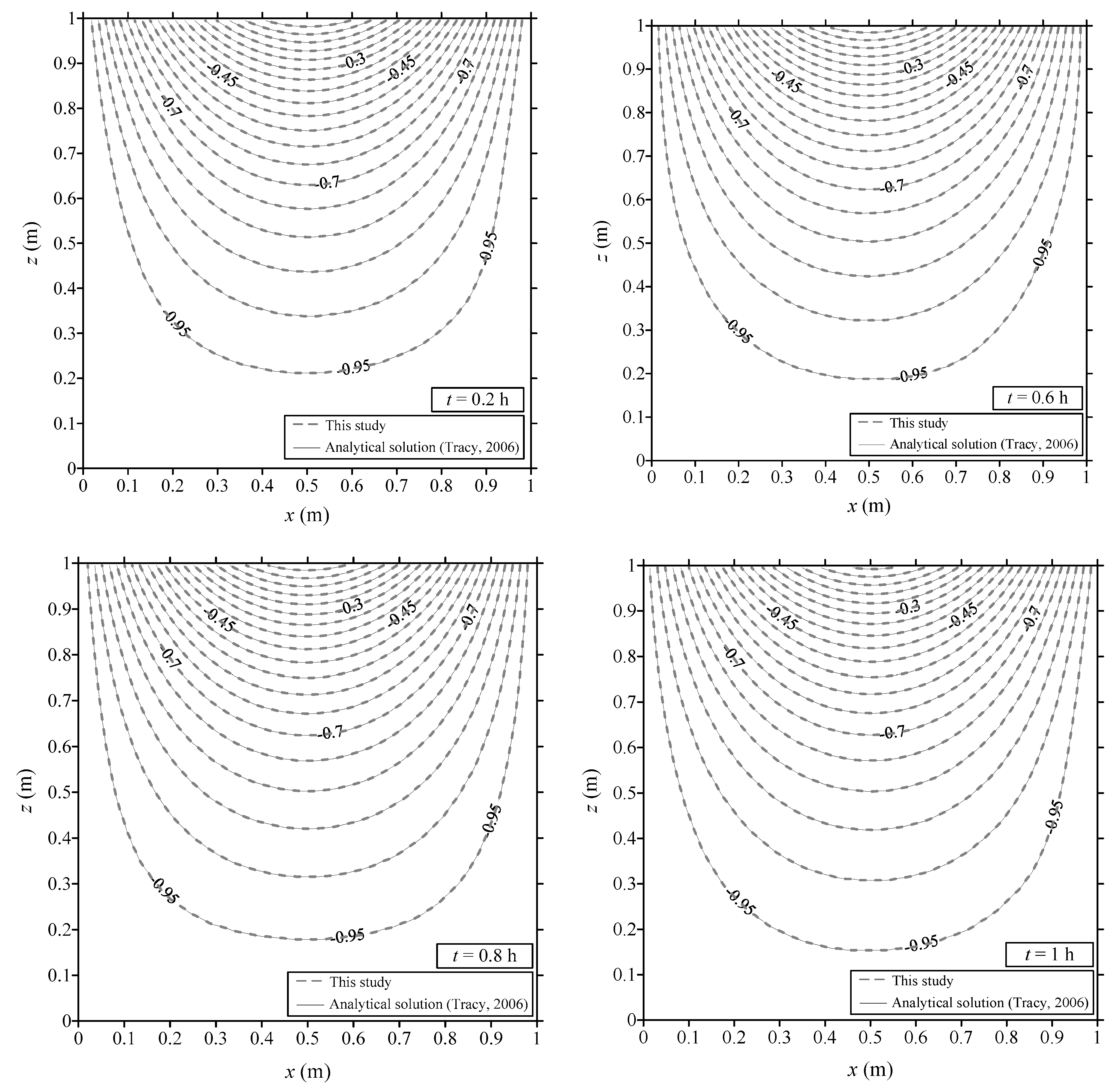
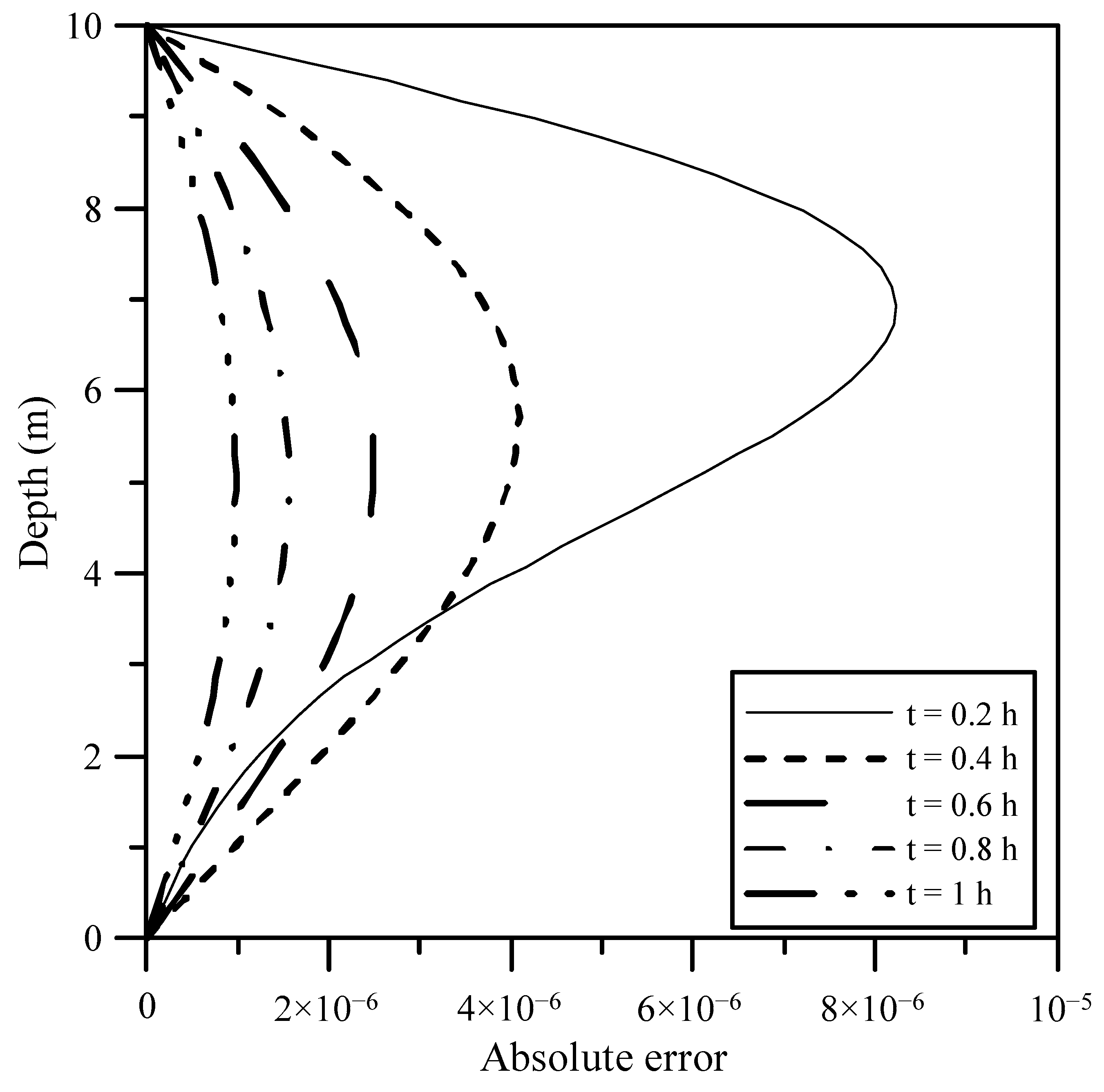
To obtain the computed results of the pressure head at different time, we collocated 2496 inner points which uniformly placed inside the rectangular domain. To view the results clearly, the profiles of the numerical solution on different time were selected to compare with the analytical solution. Figure 7 indicates that the computed results agreed very well with the analytical solution. Results obtained demonstrates that the accuracy of the absolute error can be reached to the order of . The above numerical example also illustrates that the transient problem can be solved without using the traditional time-marching scheme.
The previous example has validated the one-dimensional transient unsaturated flow problem with the analytical solution. We further investigated the application of the one-dimensional transient Green–Ampt problem using the proposed method. A column of soil is initially dry until water begins to infiltrate the soil. A pool of water at ground surface is then maintained holding the pressure head to zero. This is known as the one-dimensional Green–Ampt problem [53].
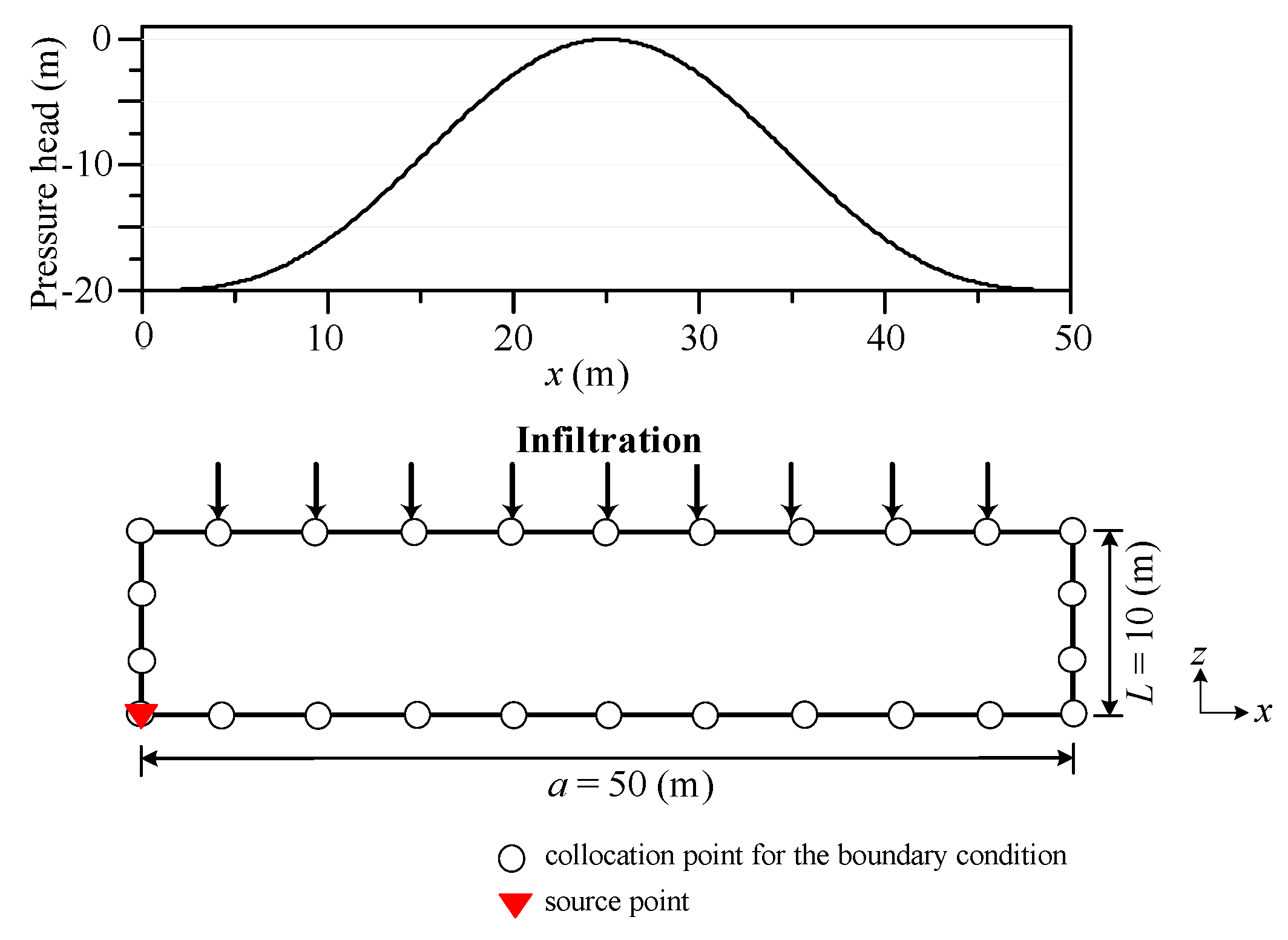
The thickness of the soil (L) is 10 (m). The soil parameters including , , and are the same as previous one. The total simulation time is 1 h. The governing equation is the same as shown in Equation (52). The initial condition is also the same as shown in Equation (53), where the soil is in dry condition maintained as .
At time greater than zero, the boundary conditions at top and bottom of the soil can be expressed as follows.
The solution procedure is similar with the previous one which also adopted the coordinate system in Minkowski spacetime. The imposed initial condition was applied on the left side of the domain and the imposed boundary conditions were applied on both top and bottom sides of the domain. By selecting (m) and (h), there are 375 boundary collocation points and a source point. The Dirichlet boundary values from the given initial and boundary conditions were given on boundary collocation points which collocated on three sides of the spacetime domain. We selected and for solving this example.
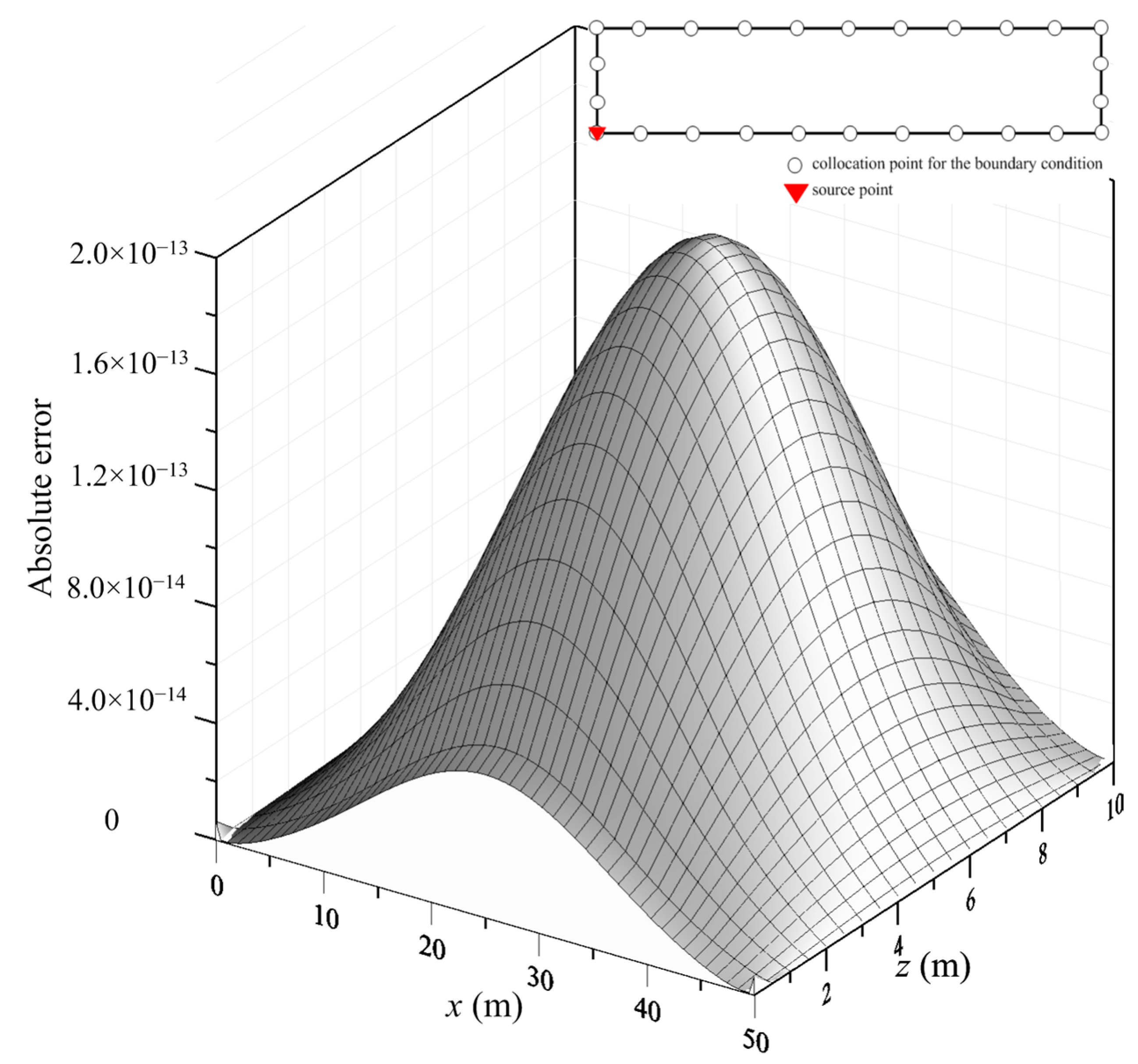
To obtain the computed results of the pressure head at different time, we collocated 2496 inner points which uniformly placed inside the rectangular spacetime domain. Figure 8 demonstrates the absolute error of this example which demonstrates that the accuracy can be reached to the order of .
3.3. Transient Modeling of Two-Dimensional Flow in Unsaturated Soil
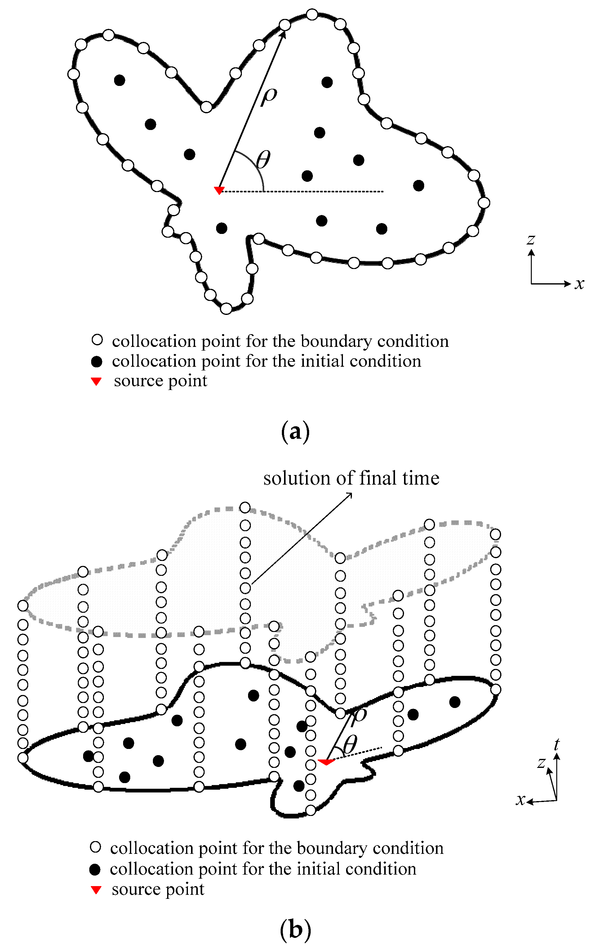
The third example under investigation is the transient modeling of two-dimensional flow in unsaturated soil. With a two-dimensional simply connected domain, , enclosed by amoeba-like boundary, as shown in Figure 9a, the governing equation can be expressed as Equation (5). The linearized Richards equation is expressed as Equation (10). The soil parameters including , , and are the same as previous one. The total simulation time is one (h). The initial condition was the soil in dry condition maintained as . Thus,
A two-dimensional amoeba-like object boundary under consideration is defined as
where .
The boundary conditions are assumed to be the Dirichlet boundary condition. The Dirichlet boundary data are applied using the following analytical solution.
The can be obtained using the following equations.
Finally, the transient solution can be obtained as follows.
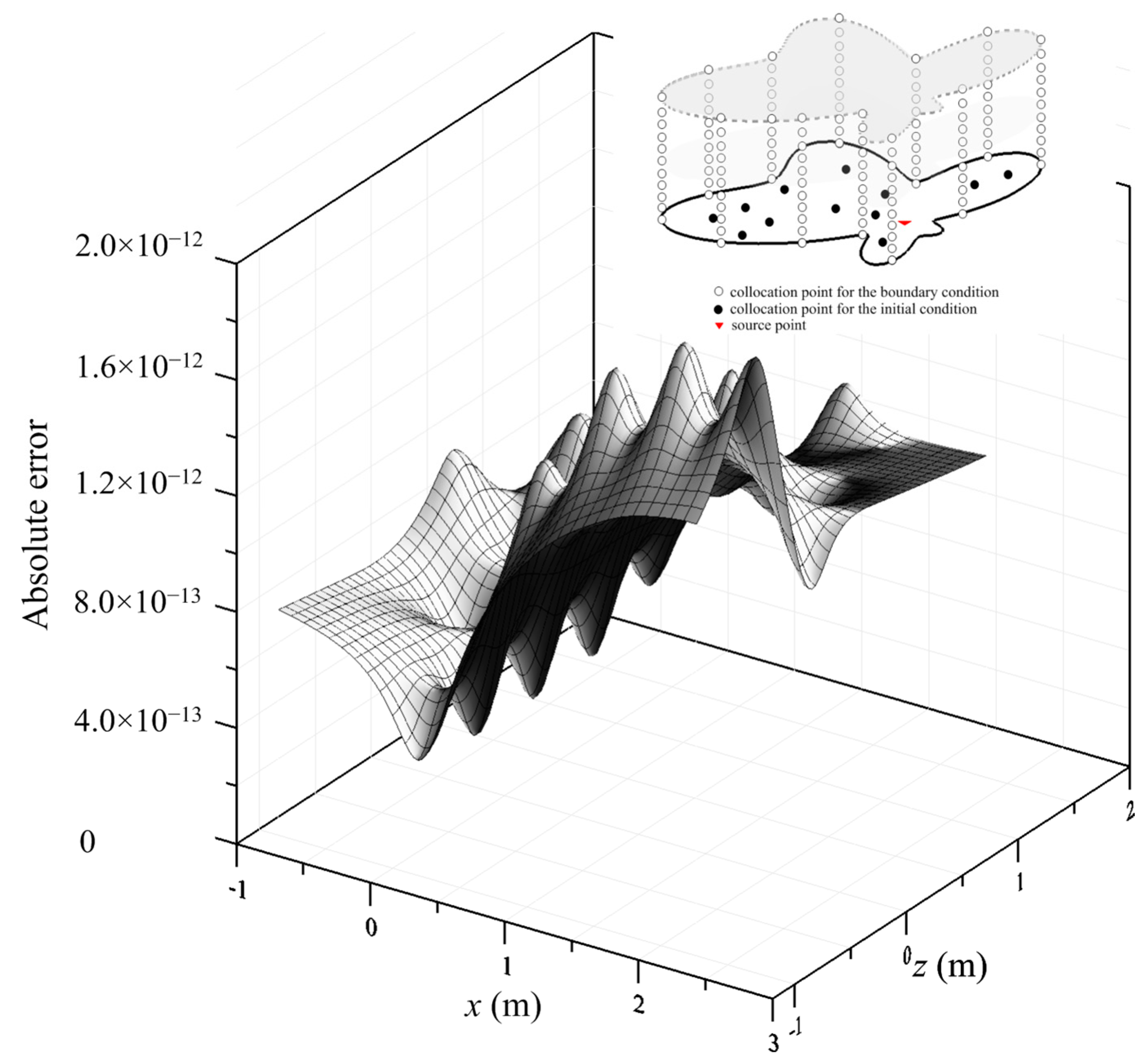
To deal with the transient modeling of two-dimensional flow in unsaturated soil, we again adopted the coordinate system in Minkowski spacetime instead of that in the original Euclidean space. In this example, there is two-dimensional space and one-dimensional time. The spacetime domain is therefore transformed a three-dimensional amoeba-like object domain, as shown in Figure 9b. We transformed the two-dimensional initial value problem into the three-dimensional inverse boundary value problem because the top side boundary values were not assigned, as depicted in Figure 9b. The initial condition was applied on the bottom side of the spacetime domain and the boundary conditions were applied on the circumferential amoeba-like boundary.
There are 3028 boundary collocation points and a source point. The Dirichlet boundary values from the given initial and boundary conditions were given on boundary collocation points which collocated on bottom and circumferential amoeba-like boundaries of the spacetime domain. We selected , and for solving this example.
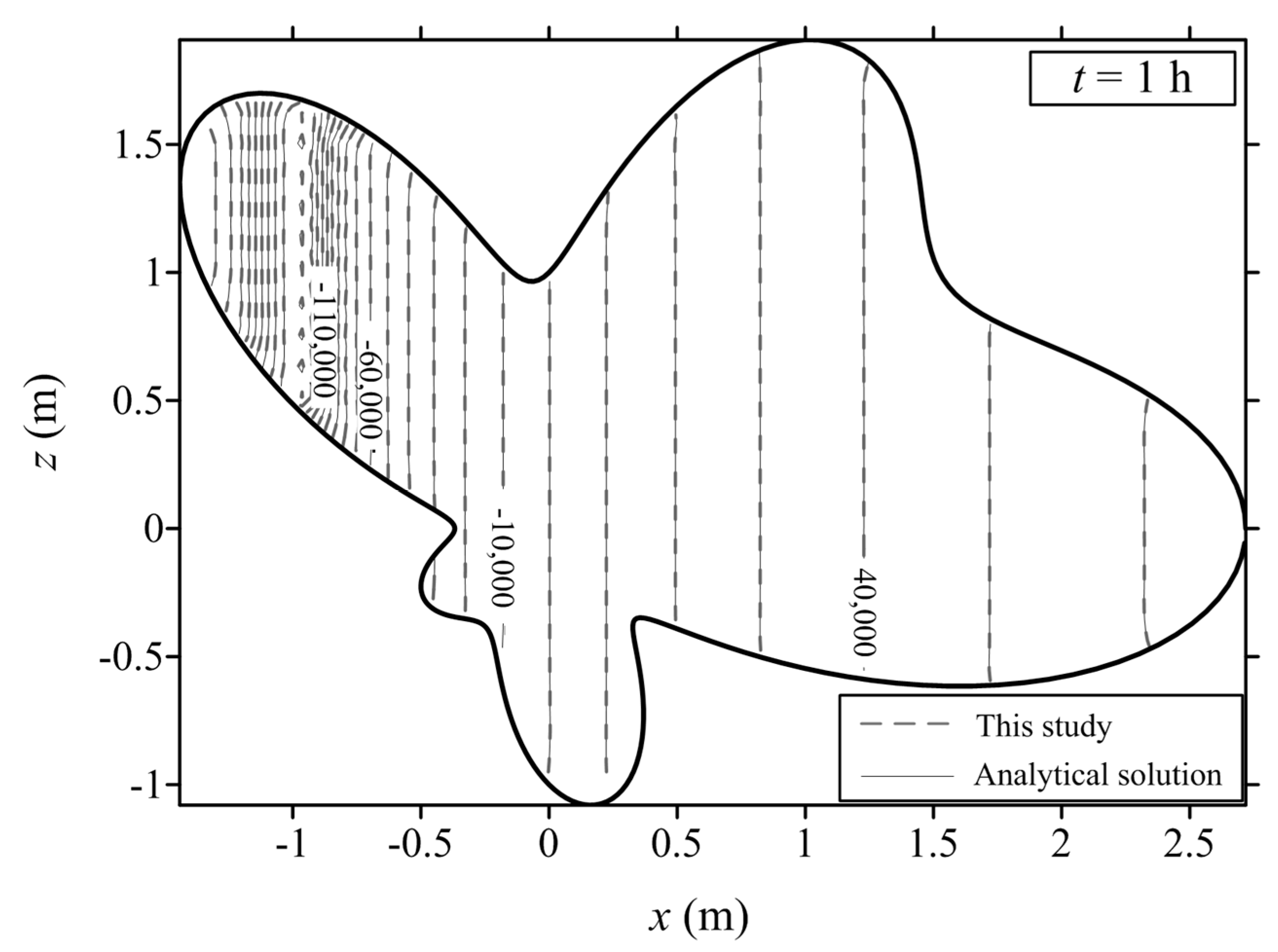
To obtain the computed results of the pressure head at different time, we collocated 370 inner points which uniformly placed inside the three-dimensional spacetime domain. Figure 10 illustrates that the computed results agreed very well with the analytical solution. Figure 11 indicates the absolute error of the two-dimensional computed results. It is found that highly accurate numerical solutions in the order of can be obtained for this example.
The previous example has validated the two-dimensional transient unsaturated flow problem with the analytical solution. We further investigated the application of the two-dimensional transient Green–Ampt problem using the proposed method. Figure 12a shows a two-dimensional cross section of a soil with the dimensions of length and height . The soil parameters including , , and are the same as previous one. The total simulation time is 1 h. This is known as the two-dimensional Green–Ampt problem. The soil is initially dry until infiltration is supplied such that a specified pressure head is applied at the top with pressure set to zero in the center and tapering rapidly to dry condition at two sides of the boundary. The specified pressure head boundary condition, as shown in Equation (70), is applied at the top of the soil. The bottom, left and right sides of the soil are in dry condition maintained as , as depicted in Figure 12a.
The governing equation is the same as shown in Equation (5). The linearized Richards equation is expressed as Equation (10). The initial condition was assumed to be dry. Thus,
The boundary conditions of the soil are as follows.
The analytical solution [46] for can be expressed as
Finally, the transient solution can be obtained using Equations (63)–(65). The solution procedure is similar with the previous one which also adopted the coordinate system in Minkowski spacetime. The imposed initial condition was applied on the bottom side of the domain and the imposed boundary conditions were applied on all four vertical sides of the domain, as shown in Figure 12b. By selecting (m) and (h), there are 736 boundary collocation points and a source point. The Dirichlet boundary values from the given initial and boundary conditions were given on boundary collocation points which collocated on five sides of the spacetime domain. We selected , and for solving this example.
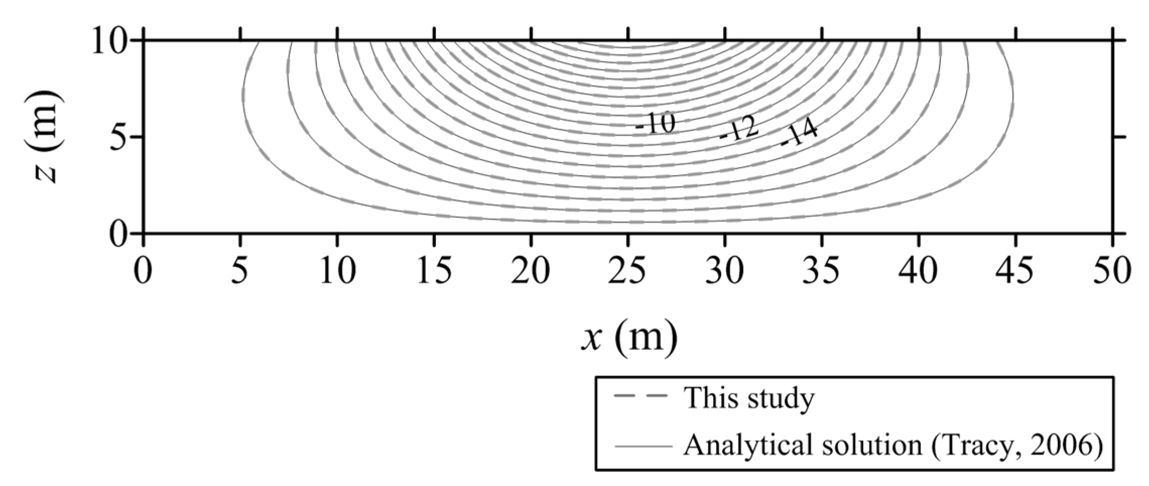
To obtain the results of the pressure head at different time, we collocated 4056 inner points which uniformly placed inside the cubic spacetime domain. Results obtained demonstrate that the numerical solution agreed very well with the analytical solution, as depicted in Figure 13. It is found that the accuracy can be reached to the order of . The above numerical example also illustrates that the two-dimensional transient unsaturated flow problem can be solved without using the traditional time-marching scheme.
4. Conclusions
This study has proposed a novel meshless method for the transient modeling of subsurface flow in unsaturated soils. This pioneering study is based on the CTM and provides a promising solution for transient modeling of subsurface flow in unsaturated soils. The validity of the model is established for a number of test problems. Application examples of subsurface flow problems in unsaturated soils were also carried out. The fundamental concepts and the construct of the proposed method are addressed in detail. The findings are addressed as follows.
It is well known that the Richards equation is a highly nonlinear equation governed by nonlinear physical relationships. In this study, we proposed a linearization process using the Gardner exponential model for the nonlinear Richards equation to model the subsurface flow in unsaturated soils. As a result, the CTM can be applied to the numerical modeling of subsurface flow in unsaturated soils.
The CTM is originally developed to deal with the boundary value problems. The pioneering work in this study is the first successful attempt to solve the transient problem using the CTM. For the transient modeling of the subsurface flow in unsaturated soils, we proposed an innovated concept that one may adopt the coordinate system in Minkowski spacetime instead of that in the original Euclidean space. Consequently, both the initial and boundary conditions can be treated as boundary conditions on the spacetime domain boundary. The initial value problem for transient modeling of subsurface flow in unsaturated soils can then be transformed into the inverse boundary value problem. As a result, the transient problems can be solved without using the traditional time-marching scheme.
Results obtained from examples revealed that the proposed method could be easily applied to one-dimensional and two-dimensional subsurface flow problems in unsaturated soils. Since the proposed CTM is a boundary-type meshless method, it is advantageous, especially for problems involving regions of irregular geometry. In addition, the proposed method can yield highly accurate numerical solutions. The results of this study demonstrate that the applicability of the CTM may be extended to other major engineering problems in the near future.
Acknowledgments
This study was partially supported by the Ministry of Science and Technology of Taiwan under project grant MOST 106-2621-M-019-004-MY2. The authors thank the Ministry of Science and Technology of Taiwan for the generous financial support.
Author Contributions
Cheng-Yu Ku worked on the conceptualization and finalized the manuscript; Chih-Yu Liu worked on the mathematical development and numerical computations; Jing-En Xiao analyzed the data; and Weichung Yeih supervised the research.
Conflicts of Interest
The authors declare no conflict of interest.
References
- Sinai, G.; Dirksen, C. Experimental evidence of lateral flow in unsaturated homogeneous isotropic sloping soil due to rainfall. Water Resour. Res. 2006, 42, W12402. [Google Scholar] [CrossRef]
- Ebel, B.A. Simulated unsaturated flow processes after wildfire and interactions with slope aspect. Water Resour. Res. 2013, 49, 8090–8107. [Google Scholar] [CrossRef]
- Ku, C.Y.; Liu, C.Y.; Su, Y.; Xiao, J.E.; Huang, C.C. Transient modeling of regional rainfall-triggered shallow landslides. Environ. Earth Sci. 2017, 76, 1–18. [Google Scholar] [CrossRef]
- Huang, F.; Luo, X.; Liu, W. Stability analysis of hydrodynamic pressure landslides with different permeability coefficients affected by reservoir water level fluctuations and rainstorms. Water 2017, 9, 450. [Google Scholar] [CrossRef]
- Richards, L.A. Capillary conduction of liquids through porous mediums. J. Appl. Phys. 1931, 1, 318–333. [Google Scholar] [CrossRef]
- Brooks, R.H.; Corey, A.T. Hydraulic Properties of Porous Media; Hydrology Paper No. 3; Colorado State University: Fort Collins, CO, USA, 1964; p. 27. [Google Scholar]
- Van Genuchten, M.T. A closed form equation for predicting the hydraulic conductivity of unsaturated soils. Soil Sci. Soc. Am. J. 1980, 44, 892–898. [Google Scholar] [CrossRef]
- Fredlund, D.G.; Xing, A.; Huang, S. Predicting the permeability function for unsaturated soils using the soil-water characteristic curve. Can. Geotech. J. 1994, 31, 533–546. [Google Scholar] [CrossRef]
- Haverkamp, R.; Vauclin, M.; Touma, J.; Wierenga, P.J.; Vachaud, G. A comparison of numerical simulation models for one dimensional infiltration. Soil Sci. Soc. Am. J. 1977, 41, 285–294. [Google Scholar] [CrossRef]
- Kavetski, D.; Binning, P.; Sloan, S.W. Noniterative time stepping schemes with adaptive truncation error control for the solution of Richards equation. Water Resour. Res. 2002, 38. [Google Scholar] [CrossRef]
- Miller, C.T.; Abhishek, C.; Farthing, M.W. A spatially and temporally adaptive solution of Richards’ equation. Adv. Water Resour. 2006, 29, 525–545. [Google Scholar] [CrossRef]
- Li, H.; Farthing, M.W.; Dawson, C.N.; Miller, C.T. Local discontinuous Galerkin approximations to Richards’ equation. Adv. Water Resour. 2007, 30, 555–575. [Google Scholar] [CrossRef]
- Juncu, G.; Nicola, A.; Popa, C. Nonlinear multigrid methods for numerical solution of the variably saturated flow equation in two space dimensions. Transp. Porous Media 2012, 91, 35–47. [Google Scholar] [CrossRef]
- Carbone, M.; Brunetti, G.; Piro, P. Modelling the Hydraulic behaviour of growing media with the explicit finite volume solution. Water 2015, 7, 568–591. [Google Scholar] [CrossRef]
- Liu, X.; Zhan, H. Calculation of steady-state evaporation for an arbitrary matric potential at bare ground surface. Water 2017, 9, 729. [Google Scholar] [CrossRef]
- Celia, M.A.; Ahuja, L.R.; Pinder, G.F. Orthogonal collocation and alternating- direction procedures for unsaturated flow problems. Adv. Water Resour. 1987, 10, 178–187. [Google Scholar] [CrossRef]
- Celia, M.A.; Bouloutas, E.T.; Zarba, R.L. A General mass-conservation numerical solution for the unsaturated flow equation. Water Resour. Res. 1990, 26, 1483–1496. [Google Scholar] [CrossRef]
- Chen, F.; Ren, L. Application of the finite difference heterogeneous multiscale method to the Richards’ equation. Water Resour. Res. 2008, 44. [Google Scholar] [CrossRef]
- Liu, C.Y.; Ku, C.Y.; Huang, C.C.; Lin, D.G.; Yeih, W. Numerical solutions of groundwater flow in unsaturated layered soil with extreme physical property contrasts. Int. J. Nonlinear Sci. Numer. Simul. 2015, 16, 325–336. [Google Scholar] [CrossRef]
- Pan, L.; Warrick, A.W.; Wierenga, P.J. Finite elements methods for modeling water flow in variably saturated porous media: Numerical oscillation and mass distributed schemes. Water Resour. Res. 1996, 32, 1883–1889. [Google Scholar] [CrossRef]
- Bergamaschi, L.; Putti, M. Mixed finite elements and Newton-type linearizations for the solution of Richards’ equation. Int. J. Numer. Methods Eng. 1999, 45, 1025–1046. [Google Scholar] [CrossRef]
- Farthing, M.W.; Kees, C.E.; Miller, C.T. Mixed finite element methods and higher order temporal approximations for variably saturated groundwater flow. Adv. Water Resour. 2003, 26, 373–394. [Google Scholar] [CrossRef]
- Bause, M.; Knabner, P. Computation of variably saturated subsurface flow by adaptive mixed hybrid finite element methods. Adv. Water Resour. 2004, 27, 565–581. [Google Scholar] [CrossRef]
- Katsurada, M.; Okamoto, H. The collocation points of the fundamental solution method for the potential problem. Comput. Math. Appl. 1996, 31, 123–137. [Google Scholar] [CrossRef]
- Liu, C.S. A modified collocation Trefftz method for the inverse Cauchy problem of Laplace equation. Eng. Anal. Bound. Elem. 2008, 32, 778–785. [Google Scholar] [CrossRef]
- Chang, Y.S.; Chang, T.J. SPH simulations of solute transport in flows with steep velocity and concentration gradients. Water 2017, 9, 132. [Google Scholar] [CrossRef]
- Yeih, W.; Chan, I.Y.; Ku, C.Y.; Fan, C.M. Solving the inverse Cauchy problem of the Laplace equation using the method of fundamental solutions and the exponentially convergent scalar homotopy algorithm (ECSHA). J. Mar. Sci. Technol. 2015, 23, 162–171. [Google Scholar]
- Huyakorn, P.S.; Pinder, G.F. Computational Methods in Subsurface Flow; Academic Press: London, UK, 1983; pp. 354–401. ISBN 978-0-12-363480-1. [Google Scholar]
- Liu, C.S. A modified Trefftz method for two-dimensional Laplace equation considering the domain’s characteristic length. Comput. Model. Eng. Sci. 2007, 1, 53–65. [Google Scholar]
- Trefftz, E. Ein gegenstück zum ritzschen verfahren. In Proceedings of the 2nd International Congress for Applied Mechanics, Zurich, Switzerland, 12–17 September 1926; pp. 131–137. [Google Scholar]
- Kita, E.; Kamiya, N. Trefftz method: An overview. Adv. Eng. Softw. 1995, 24, 3–12. [Google Scholar] [CrossRef]
- Kupradze, V.D.; Aleksidze, M.A. The method of functional equations for the approximate solution of certain boundary value problems. Comput. Math. Math. Phys. 1964, 4, 82–126. [Google Scholar] [CrossRef]
- Chen, C.S.; Karageorghis, A.; Li, Y. On choosing the location of the sources in MFS. Numer. Algorithms 2016, 72, 107–130. [Google Scholar] [CrossRef]
- Belytschko, T.; Lu, Y.Y.; Gu, L. Element free Galerkin methods. Int. J. Numer. Methods Eng. 1994, 37, 229–256. [Google Scholar] [CrossRef]
- Liu, W.K.; Jun, S.; Zhang, Y.F. Reproducing kernel particle methods. Int. J. Numer. Methods Fluids 1995, 20, 1081–1106. [Google Scholar] [CrossRef]
- Lin, H.; Atluri, S.N. Meshless Local Petrov-Galerkin (MLPG) method for convection-diffusion problems. Comput. Model. Eng. Sci. 2000, 1, 45–60. [Google Scholar]
- Kita, E.; Ikedab, Y.; Kamiya, N. Trefftz solution for boundary value problem of three-dimensional Poisson equation. Eng. Anal. Bound. Elem. 2005, 29, 383–390. [Google Scholar] [CrossRef]
- Fan, C.M.; Chan, H.F.; Kuo, C.L.; Yeih, W. Numerical solutions of boundary detection problems using modified collocation Trefftz method and exponentially convergent scalar homotopy algorithm. Eng. Anal. Bound. Elem. 2012, 36, 2–8. [Google Scholar] [CrossRef]
- Li, Z.C.; Lu, Z.Z.; Hu, H.Y.; Cheng, H.D. Trefftz and Collocation Methods; WIT Press: Southampton, UK, 2008. [Google Scholar]
- Gardner, W.R. Some steady-state solutions of the unsaturated moisture flow equation with application to evaporation from a water table. Soil Sci. 1958, 85, 228–232. [Google Scholar] [CrossRef]
- Srivastava, R.; Yeh, T.-C.J. Analytical solutions for onedimensional, transient infiltration toward the water table in homogeneous and layered soils. Water Resour. Res. 1991, 27, 753–762. [Google Scholar] [CrossRef]
- Galison, P.L. Minkowski’s Space-Time: From visual thinking to the absolute world. Hist. Stud. Phys. Sci. 1979, 10, 85–121. [Google Scholar] [CrossRef]
- Naber, G.L. The Geometry of Minkowski Spacetime; Springer-Verlag: New York, NY, USA, 1992. [Google Scholar]
- Catoni, F.; Boccaletti, D.; Cannata, R.; Catoni, V.; Nichelatti, E.; Zampetti, P. The Mathematics of Minkowski Space-Time with an Introduction to Commutative Hypercomplex Numbers; Birkhäuser Verlag: Basel, Switzerland, 2008; pp. 5–17. ISBN 978-3-7643-8613-9. [Google Scholar]
- Segol, G. Classic Groundwater Simulations; Prentice Hall: Englewood Cliffs, NJ, USA, 1994. [Google Scholar]
- Tracy, F.T. Clean two- and three-dimensional analytical solutions of Richards’ equation for testing numerical solvers. Water Resour. Res. 2006, 42. [Google Scholar] [CrossRef]
- Kita, E.; Kamiya, N.; Iio, T. Application of a direct Trefftz method with domain decomposition to two-dimensional potential problems. Eng. Anal. Bound. Elem. 1999, 23, 539–548. [Google Scholar] [CrossRef]
- Yeih, W.; Liu, C.S.; Kuo, C.L.; Atluri, S.N. On solving the direct/inverse cauchy problems of laplace equation in a multiply connected domain, using the generalized multiple-source-point boundary-collocation Trefftz method and characteristic lengths. Comput. Mater. Contin. 2010, 17, 275–302. [Google Scholar]
- Ku, C.Y. On solving three-dimensional Laplacian problems in a multiply connected domain using the multiple scale Trefftz method. Comput. Model. Eng. Sci. 2014, 98, 509–541. [Google Scholar]
- Ku, C.Y.; Kuo, C.L.; Fan, C.M.; Liu, C.S.; Guan, P.C. Numerical solution of three-dimensional Laplacian problems using the multiple scale Trefftz method. Eng. Anal. Bound. Elem. 2015, 50, 157–168. [Google Scholar] [CrossRef]
- Ku, C.Y.; Xiao, J.E.; Liu, C.Y.; Yeih, W. On the accuracy of the collocation Trefftz method for solving two and three dimensional heat equations. Numer. Heat Transf. Part B 2016, 69, 334–350. [Google Scholar] [CrossRef]
- Logan, J.D. Applied Mathematics; John Wiley & Sons, Inc.: Hoboken, NJ, USA, 1987; pp. 275–360. ISBN 9780471165132. [Google Scholar]
- Green, W.H.; Ampt, G.A. Studies on soil physics I. The flow of air and water through soils. J. Agric. Sci. 1911, 4, 1–24. [Google Scholar]
- Lu, N.; Likos, W.J. Unsaturated Soil Mechanics; John Wiley & Sons, Inc.: Hoboken, NH, USA, 2004; pp. 494–527. ISBN 0-471-44731-5. [Google Scholar]
Figure 1.
The computed pressure head distribution.
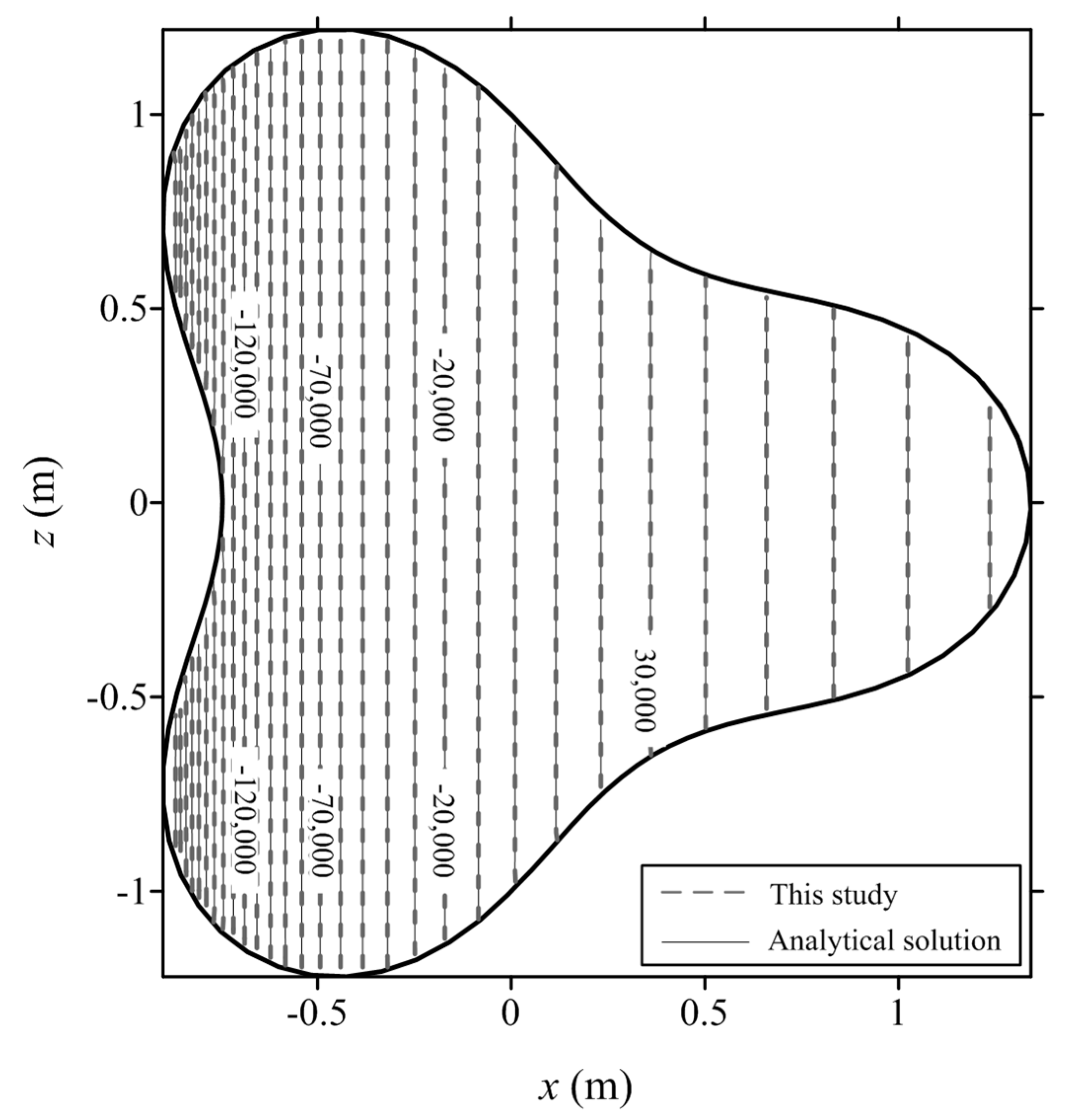
Figure 2.
The absolute error of the computed results.
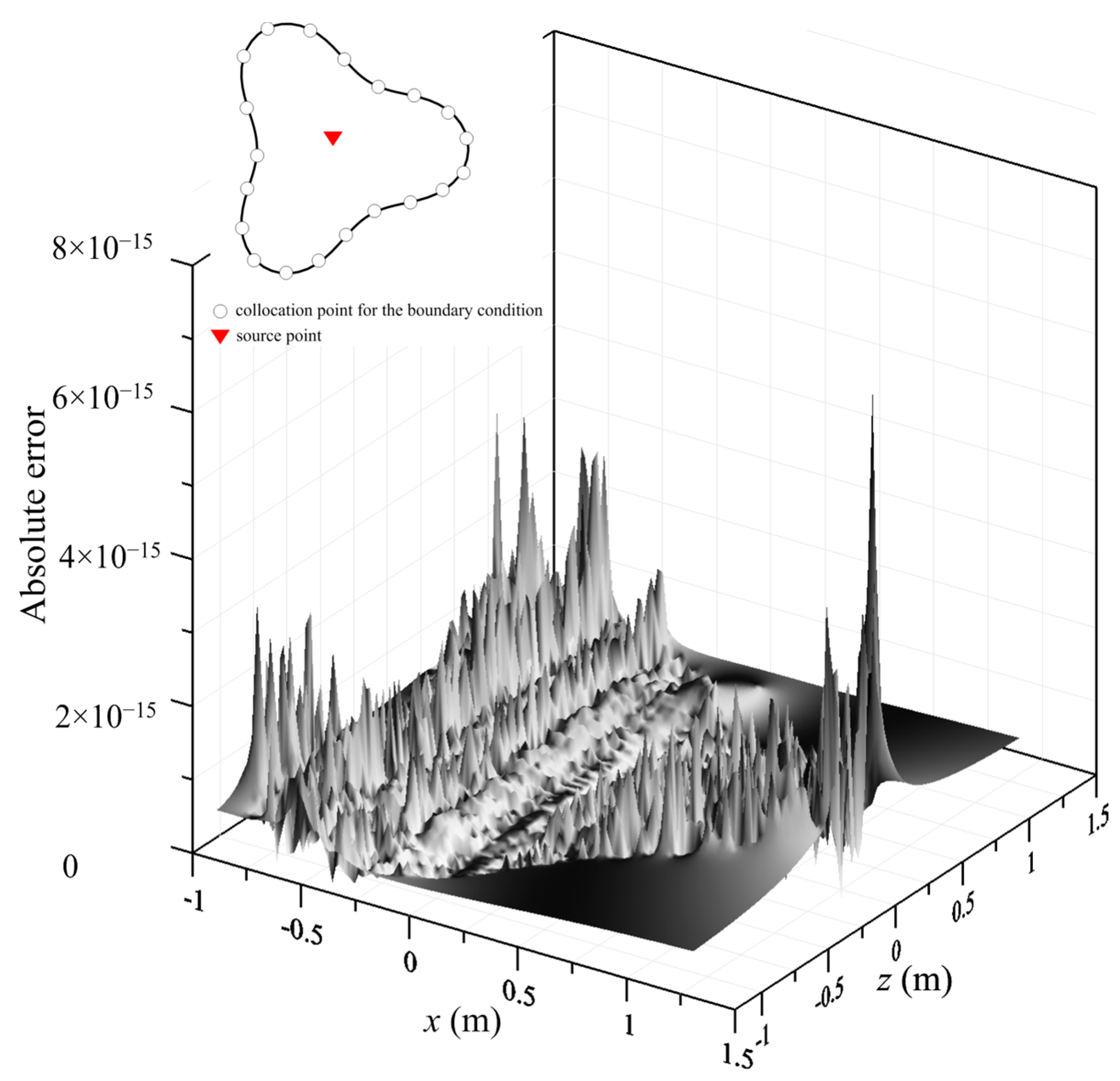
Figure 3.
A view of a two-dimensional steady-state Green–Ampt problem.

Figure 4.
Comparison of computed pressure head distribution with the analytical solution for the two-dimensional steady-state Green–Ampt problem.
Figure 4.
Comparison of computed pressure head distribution with the analytical solution for the two-dimensional steady-state Green–Ampt problem.

Figure 5.
The absolute error of the computed results for the two-dimensional steady-state Green–Ampt problem.
Figure 5.
The absolute error of the computed results for the two-dimensional steady-state Green–Ampt problem.

Figure 6.
Illustration of the collocation scheme for the Trefftz method in Minkowski spacetime for the one-dimensional transient problem: (a) original one-dimensional transient problem (one-dimensional initial value problem); and (b) collocation points of one-dimensional transient problem in Minkowski spacetime domain (two-dimensional inverse boundary value problem).


Figure 7.
Comparison of the computed results with the analytical solution.
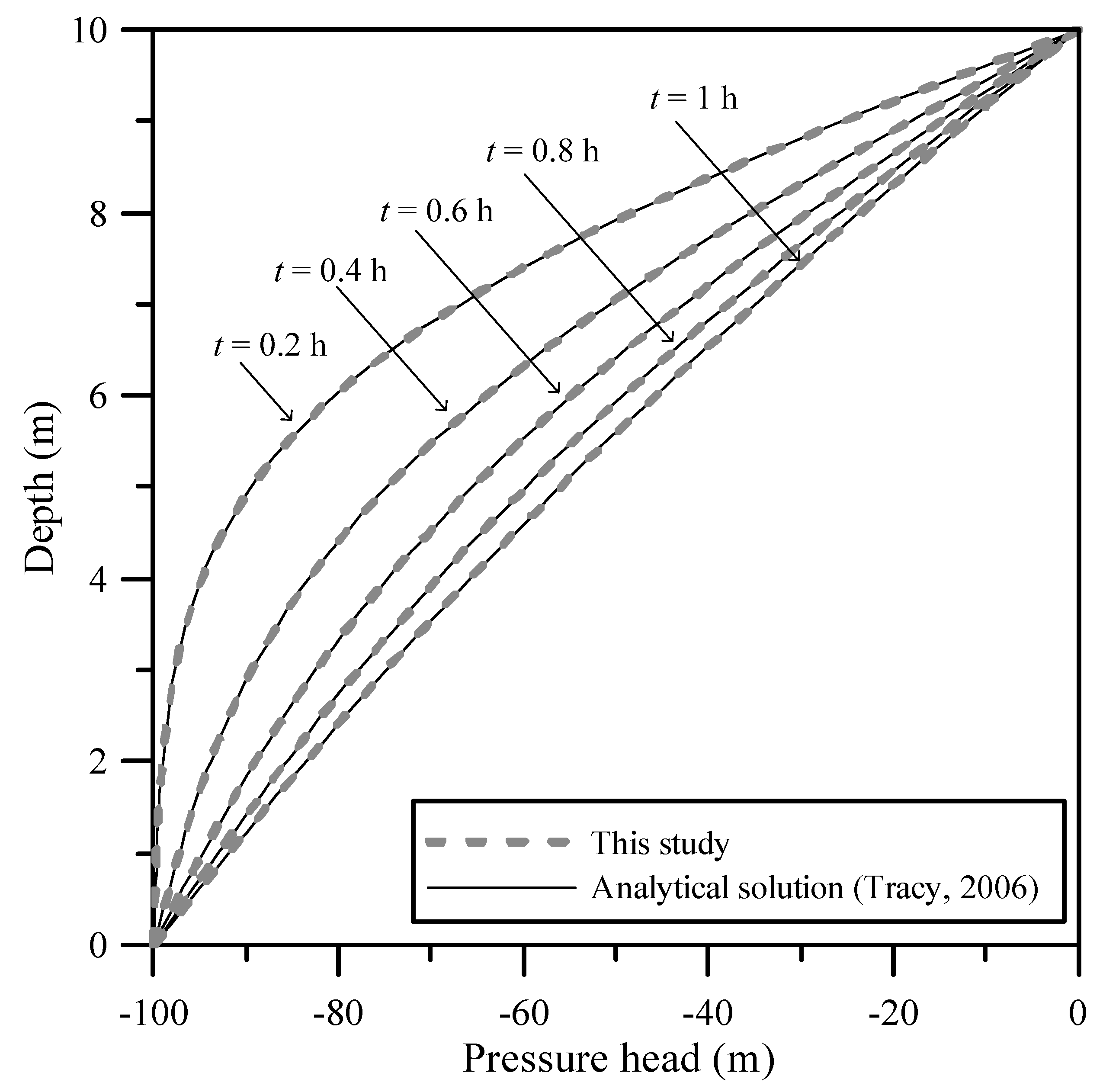
Figure 8.
The absolute error of the computed results for the transient modeling of the one-dimensional Green–Ampt problem.
Figure 8.
The absolute error of the computed results for the transient modeling of the one-dimensional Green–Ampt problem.

Figure 9.
Schematic illustration of the two-dimensional transient flow in unsaturated soils for an amoeba-like boundary: (a) original two-dimensional transient problem (two-dimensional initial value problem); and (b) collocation points of two-dimensional transient problem in Minkowski spacetime domain (three-dimensional inverse boundary value problem).

Figure 10.
Comparison of computed results with the analytical solution for the transient modeling of the two-dimensional flow in unsaturated soils.
Figure 10.
Comparison of computed results with the analytical solution for the transient modeling of the two-dimensional flow in unsaturated soils.

Figure 11.
The absolute error of the computed results.

Figure 12.
Schematic illustration of the two-dimensional transient Green–Ampt problem: (a) original two-dimensional transient problem (two-dimensional initial value problem); and (b) collocation points of two-dimensional transient problem in Minkowski spacetime domain (three-dimensional inverse boundary value problem).
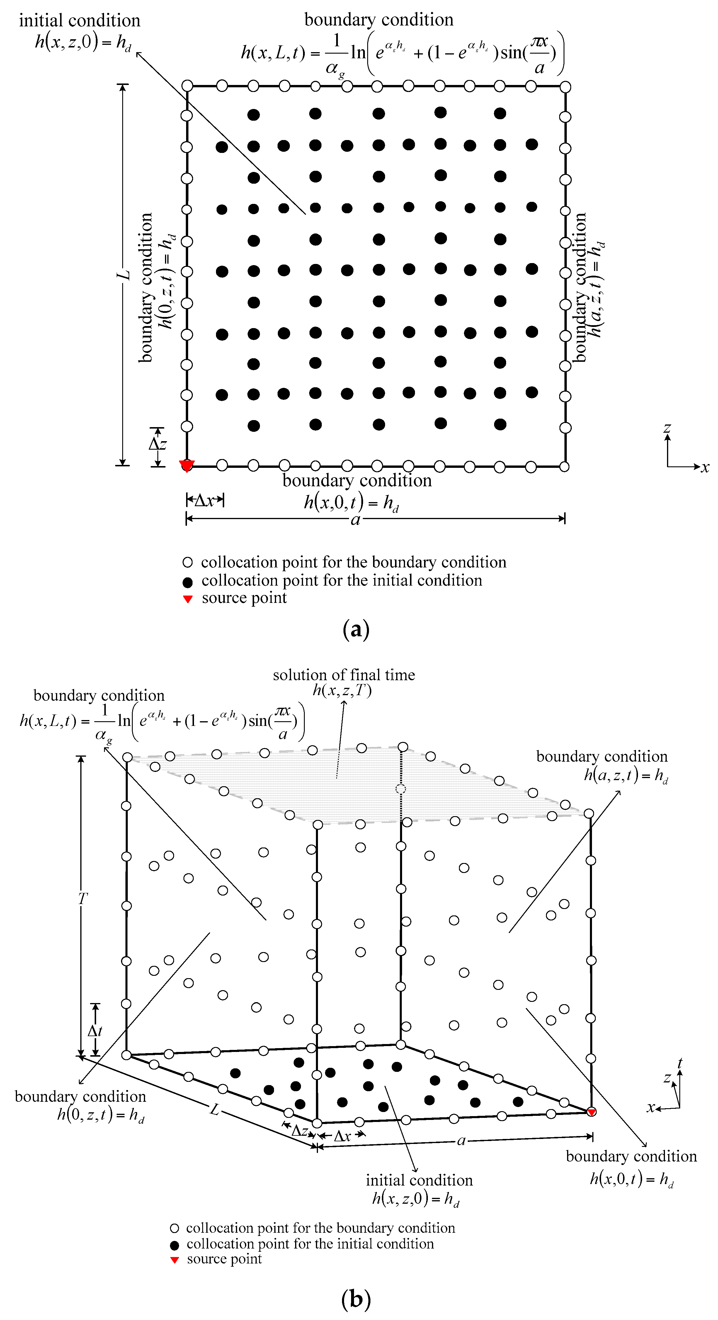
Figure 13.
Comparison of computed results with those from the analytical solution for the two-dimensional transient Green–Ampt problem.
Figure 13.
Comparison of computed results with those from the analytical solution for the two-dimensional transient Green–Ampt problem.

Table 1.
T basis functions for two-dimensional linearized Richards equation.
| Variable | Function | |
|---|---|---|
| Steady-State | ||
| Transient | ||
, | ||
Table 2.
T basis functions for one-dimensional linearized Richards equation.
| Variable | Function | |
|---|---|---|
| Transient | ||
© 2017 by the authors. Licensee MDPI, Basel, Switzerland. This article is an open access article distributed under the terms and conditions of the Creative Commons Attribution (CC BY) license (http://creativecommons.org/licenses/by/4.0/).
Share and Cite
MDPI and ACS Style
Ku, C.-Y.; Liu, C.-Y.; Xiao, J.-E.; Yeih, W. Transient Modeling of Flow in Unsaturated Soils Using a Novel Collocation Meshless Method. Water 2017, 9, 954. https://doi.org/10.3390/w9120954
AMA Style
Ku C-Y, Liu C-Y, Xiao J-E, Yeih W. Transient Modeling of Flow in Unsaturated Soils Using a Novel Collocation Meshless Method. Water. 2017; 9(12):954. https://doi.org/10.3390/w9120954
Chicago/Turabian StyleKu, Cheng-Yu, Chih-Yu Liu, Jing-En Xiao, and Weichung Yeih. 2017. "Transient Modeling of Flow in Unsaturated Soils Using a Novel Collocation Meshless Method" Water 9, no. 12: 954. https://doi.org/10.3390/w9120954
Note that from the first issue of 2016, this journal uses article numbers instead of page numbers. See further details here.