Groundwater Flow Determination Using an Interval Parameter Perturbation Method

Abstract

Groundwater flow simulation often inevitably involves uncertainty, which has been quantified by a host of methods including stochastic methods and statistical methods. Stochastic methods and statistical methods face great difficulties in applications. One of such difficulties is that the statistical characteristics of random variables (such as mean, variance, covariance, etc.) must be firstly obtained before the stochastic methods can be applied. The dilemma is that one is often unclear about such statistical characteristics, given the limited available data. To overcome the problems met by stochastic methods, this study provides an innovative approach in which the hydrogeological parameters and sources and sinks of groundwater flow are represented by bounded but uncertain intervals of variables called interval of uncertainty variables (IUVs) and this approach is namely the interval uncertain method (IUM). IUM requires only the maximum and minimum values of the variable. By utilizing the natural interval expansion, an interval-based parametric groundwater flow equation is established, and the solution of that equation can be found. Using a hypothetical steady-state flow case as an example, one can see that when the rate of change is less than 0.2, the relative error of this method is generally limited to less than 5%; when the rate of change is less than 0.3, the relative error of this method can be kept within 10%. This research shows that the proposed method has smaller relative errors and higher computational efficiency than the Monte Carlo methods. It is possible to use this method to analyze the uncertainties of groundwater flow when it is difficult to obtain the statistical characteristics of the hydrogeological systems. The proposed method is applicable in linear groundwater flow system. Its validity in nonlinear flow systems such as variably saturated flow or unconfined flow with considerable variation of water table will be checked in the future.

1. Introduction

Over the past 40 years, numerical models of groundwater flow and solute transport have been widely used in studies of water resources management, migration of pollutants, sea water intrusion and many other applications [1,2,3,4]. However, because of the complexity of hydrogeological conditions and the limited budget and time, scientists often find it difficult to collect sufficient data to completely describe the hydrogeological systems in great details. Lack of hydrogeological data will inevitably affect the reliability of the model simulations and result in model uncertainty. Therefore, how to describe the uncertainty of model inputs and outputs and to improve the reliability of model predictions has become an important element of the numerical simulations used in studies of groundwater flow and solute transport [5,6,7,8,9].

Stochastic method based on a certain statistical structure is one of the most important methods currently used to study the uncertainty of numerical models of groundwater flow [2,3,4,5,6,7,8,9]. Stochastic methods include a host of mathematical methods such as the traditional random methods [7,8] and the Bayesian statistical methods [9]. The traditional random methods mainly include the Monte Carlo (MC) method, the moment equation method and Taylor expansion method or the perturbation expansion method. The Bayesian method is a widely used stochastic method in recent decades.

The MC method is first widely used to obtain the statistical characteristics of groundwater head or solute concentrations by random sampling after the probability density function (PDF) of the hydrogeological elements is known, where the hydrogeological elements refer to the aquifer parameters such as hydraulic conductivity or transmissivity, storativity, porosity, dispersivity, etc., boundary and initial conditions of flow and transport, and sinks and sources of flow and transport [10,11,12,13]. The moment equation method can be used to calculate the mean and variance of groundwater head or solute concentrations, provided that the mean and variance of known hydrogeological elements are given [14,15,16,17,18]. The moment equation method is used to obtain the first and second moments of the hydraulic head (for flow problems) or the solute concentration (for transport problems) by the first and second moments of the stochastic governing equation. Many investigators have carried out the uncertainty analysis of numerical simulations based on the Taylor expansion method or the perturbation expansion method, which also requires the mean and variance of the hydrogeological elements [19,20]. The Taylor expansion method or the perturbation expansion method expands head or concentration around its mean value and tries to make a connection between the mean and variance of head and concentration with the mean and variance of the hydrogeological elements [21,22]. The Taylor expansion or perturbation expansion method often involves the inversion of a large coefficient matrix, which could be computationally expensive. In addition, several investigators have studied the random theory using other methods [23,24,25,26,27,28,29].

Bayesian theory has also been widely used in the uncertainty analysis of numerical simulations of groundwater flow and solute transport. This theory involves three aspects including sampling methods, likelihood functions and convergence criteria [1]. A crucial step of the Bayesian theory is the sampling algorithm. There are several commonly used sampling algorithms, such as the Metropolis-Hastings algorithm, the Gibbs algorithm and the adaptive Metropolis algorithm [30,31,32,33,34,35,36,37,38,39,40]. Bayesian theory can obtain the posterior probability density function of hydrogeological elements, but the premise is that the distribution of hydrogeological parameters is known a priori.

Based on the random statistical characteristics of the hydrogeological elements, the stochastic method obtains the statistical characteristics of the output (mainly, the head and concentration). Unfortunately, it is sometimes difficult to know the stochastic statistical characteristics of the hydrogeological elements a priori in actual applications.

However, although precise statistical characteristics of the hydrogeological elements may be difficult to obtain, it may be easier to determine the ranges of possible values for the hydrogeological elements, probably with the help hydrogeological surveys, which is conventionally conducted in nearly all the hydrogeological investigations. If this is true, now the question is: Can we quantitatively determine the ranges of system outputs, given the bounded but uncertain inputs of the hydrogeological elements? The method used to tackle this question is named the interval uncertainty method (IUM), and it is practically appealing in terms of managing groundwater resources and conducting risk assessment of contaminated aquifers. A minor point to note is that IUM has been successfully carried out in other disciplines such as structural engineering, interval optimization method, and irrigation water distribution, but has never been applied in subsurface hydrology [41,42,43,44,45,46,47,48,49,50].

This study is the first attempt to use IUM for dealing with a linear groundwater flow system in a confined aquifer. Comparison of the presented (analytic) IUM and numerical analysis of a few hypothetical examples shows that the computational efficiency and precision of this method are very well. The validity of IUM in nonlinear subsurface flow systems such as flow in variably saturated porous media or flow in an unconfined aquifer with considerable variation of water table with time is out of the scope of this study, and will be investigated in the future.

2. Problem Description

IUM involves the interval response expression whose mathematical background is briefly explained as follows.

2.1. Interval Response Expression

We consider that the groundwater system response $\omega$ is a function of the system parameters $\alpha$ = ${\left({\alpha }_1,{\alpha }_2,\dots ,{\alpha }_m\right)}^T$, as stated below.

$$\omega =\omega \left(\alpha \right)=\omega \left({\alpha }_1,{\alpha }_2,\dots ,{\alpha }_m\right),$$

(1)

where $\omega$ is a vector or scalar, m is the number of parameters, and T in the superscript is the transpose sign.

We consider that there are parameters with uncertainties in the parameter space. If we only know their uncertainty range, they can be expressed using the following interval form:

$${\alpha }^I=[\underset{\_}{\alpha },\overline{\alpha }]=\{\alpha :\underset{\_}{\alpha }\le \alpha \le \overline{\alpha },\underset{\_}{\alpha },\overline{\alpha }\in R^L\}$$

(2)

in which $\overline{\alpha }$ and $\underset{\_}{\alpha }$ are, respectively, the vectors of the upper and lower bounds of the vector of uncertain parameters $\alpha$, $R^L$ is a real vector space. When the bounded uncertain parameters or parameters vector $\mathsf{\alpha }$ change within the range represented by Equation (2), the changing range for the system response ω can be expressed in the following form:

$$\Gamma =\{\omega :\omega =\omega \alpha ,\underset{\_}{\alpha }\le \alpha \le \overline{\alpha }\}$$

(3)

When we know the upper and lower bounds of the bounded uncertain parameters or the unascertained parameter vector $\alpha$, the next task is to acquire the upper and lower bounds of the groundwater system response $\omega$, i.e., $\overline{\omega }$ and $\underset{\_}{\omega }$.

2.2. Interval Parameter Type Groundwater Head Equation

The general form of groundwater flow governing equation used in numerical simulation may be expressed as

$$KH=F$$

(4)

where K is the coefficient matrix, H is the groundwater head vector at different nodes, and F is a column vector. K and F are usually obtained by matrix and column vector superposition in a finite element or finite difference framework, i.e., K and F can be decomposed into summations as follows:

$$K=K_1+K_2+\cdots +K_m={\displaystyle \sum }_{i=1}^m{K}_i$$

(5)

$$F=F_1+F_2+\cdots +F_m={\displaystyle \sum }_{i=1}^m{F}_i$$

(6)

where m is the number of rows of K and F which are functions of hydrogeological elements, i.e.,

$$K=K\left(\alpha \right),F=F\left(\alpha \right)$$

(7)

Therefore, Equation (7) can be transformed into

$$K=K\left(\alpha \right)={\sum }_{i=1}^m{\phi }_i\left(\alpha \right)K_i^{\prime },F=F\left(\alpha \right)={\sum }_{i=1}^m{\varphi }_i\left(\alpha \right)F_i^{\prime }$$

(8)

where $K_i={\phi }_i\left(\alpha \right)K_i^{\prime },F_i={\varphi }_i\left(\alpha \right)F_i^{\prime }$, ${\phi }_i\left(\alpha \right)$ and ${\varphi }_i\left(\alpha \right)$ are functions of parameter $\alpha$, and $K_i^{\prime }\mathrm{and}{F}_i^{\prime }$ are matrix and column vector, respectively. Functions ${\phi }_i\left(\alpha \right)$ and ${\varphi }_i\left(\alpha \right)$ (i = 1, 2, …, m) may behave differently, i.e., some may be nonlinear, some may be linear, and some may be zero. If $\alpha$ denotes the hydraulic conductivity, the specific yield, the specific storage or parameters associated with the flow boundary, ${\phi }_i\left(\alpha \right)$ and ${\varphi }_i\left(\alpha \right)$ are linear functions, and Equation (8) can be simplified as

$$K=K\left(\alpha \right)={\displaystyle \sum }_{i=1}^m{\alpha }_i{K}_i^{\prime },F=F\left(\alpha \right)={\displaystyle \sum }_{i=1}^m{\alpha }_i{F}_i^{\prime }$$

(9)

If $\mathsf{\alpha }$ has an uncertainty within a specified range, $\alpha$ can be defined as ${\alpha }^I$, where ${\alpha }^I$ is the interval parameter.

$${\alpha }^I=[\underset{\_}{\alpha },\overline{\alpha }]={\alpha }_0+\mathsf{\Delta }{\alpha }^I,\mathsf{\Delta }{\alpha }^I=[-\frac{\overline{\alpha }-\underset{\_}{\alpha }}{2},\frac{\overline{\alpha }-\underset{\_}{\alpha }}{2}]$$

(10)

where ${\alpha }_0$ is the average value of parameter ${\alpha }^I$, $\overline{\alpha }-\underset{\_}{\alpha }$ is the variation of ${\alpha }^I$, and $\frac{\overline{\alpha }-\underset{\_}{\alpha }}{2{\alpha }_0}$ is the rate of change of parameter ${\alpha }^I$. According to Equation (8), we can get the following expression by utilizing the interval expansion from interval mathematics [51].

$$K\left({\alpha }_i^I\right)={\displaystyle \sum }_{i=1}^m{\alpha }_i^I{K}_i^{\prime },F\left({\alpha }_i^I\right)={\displaystyle \sum }_{i=1}^m{\alpha }_i^I{F}_i^{\prime }$$

(11)

Combining Equation (11) with Equation (10), we can also obtain the following expression.

$$K\left({\alpha }^I\right)={\sum }_{i=1}^m\left({\alpha }_i^0+\mathsf{\Delta }{\alpha }_i^I\right)K_i^{\prime },F\left({\alpha }^I\right)={\sum }_{i=1}^m\left({\alpha }_i^0+\mathsf{\Delta }{\alpha }_i^I\right)F_i^{\prime }$$

(12)

Here we can simplify Equation (12) as follows:

$$K_0={\sum }_{i=1}^m{\alpha }_i^0{K}_i^{\prime },F_0={\sum }_{i=1}^m{\alpha }_i^0{F}_i^{\prime }$$

(13)

$$\mathsf{\Delta }K=K\left(\mathsf{\Delta }{\alpha }^I\right)={\sum }_{i=1}^m\mathsf{\Delta }{\alpha }_i^I{K}_i^{\prime },\mathsf{\Delta }F=F\left(\mathsf{\Delta }{\alpha }^I\right)={\sum }_{i=1}^m\mathsf{\Delta }{\alpha }_i^I{F}_i^{\prime }$$

(14)

Finally, we can obtain the interval of groundwater head equation

$$\left(K_0+K\left(\mathsf{\Delta }{\alpha }^I\right)\right)H=F_0+F\left(\mathsf{\Delta }{\alpha }^I\right)$$

(15)

which is contained in the interval parameter $\mathsf{\Delta }{\alpha }^I$. Equation (15) is an interval algebraic equation group concerning H, whose solution is also an interval variable. Solving Equation (15), the corresponding changes of head H interval can be obtained when ${\alpha }^I$ or $\mathsf{\Delta }{\alpha }^I$ changes within a certain range.

3. Interval Response Solution

3.1. Groundwater Head Interval Response Expression

When determining the interval solution of H in Equation (15), we will first obtain the average value H₀ of H, and then calculate the variation ΔH, which is a key issue to deal with. The following discussion provides the solution to Equation (15).

The average H₀ of the groundwater head satisfies the following equation:

$$K_0{H}_0=F_0$$

(16)

where $K_0$ is the coefficient matrix when the hydrogeological parameters are set at their averages, $F_0$ is the column vector when sources and sinks take their averages as well.

Meanwhile, using $K_0+\mathsf{\Delta }K$, $H_0+\mathsf{\Delta }H$ and $F_0+\mathsf{\Delta }F$, the following equation can be written:

$$(K_0+\mathsf{\Delta }K)\left(H_0+\mathsf{\Delta }H\right)=F_0+\mathsf{\Delta }F$$

(17)

where ΔK and ΔF are respectively the variations of K and F. Considering Equations (16) and (17), and ignoring the second order and higher order terms of ΔK, ΔH, and ΔF, we can obtain an approximate expression of the first-order disturbance about the head [51].

$$\mathsf{\Delta }{H}^{\left(1\right)}=K_0^{-1}\left(\mathsf{\Delta }F-\mathsf{\Delta }K{H}_0\right)$$

(18)

where $\mathsf{\Delta }{H}^{\left(1\right)}$ is the first-order approximation of ΔH. That is, replacing ΔH with $\mathsf{\Delta }{H}^{\left(1\right)}$ in Equation (18), where H is

$$H=H_0+\mathsf{\Delta }{H}^{\left(1\right)}$$

(19)

The second-order approximation of ΔH and the corresponding H is

$$\mathsf{\Delta }{H}^{\left(2\right)}=K_0^{-1}\mathsf{\Delta }K\left(K_0^{-1}\mathsf{\Delta }F-K_0^{-1}\mathsf{\Delta }K{H}_0\right),H=H_0+\mathsf{\Delta }{H}^{\left(1\right)}+\mathsf{\Delta }{H}^{\left(2\right)}$$

(20)

According to the interval expansion from interval mathematics, substituting Equation (14) into Equation (18), the first order perturbation of ΔH is approximately

$$\mathsf{\Delta }{H}^{\left(1\right)}={\displaystyle \sum }_{i=1}^m\mathsf{\Delta }{\alpha }_i^I\left(K_0^{-1}(F_i^{\prime }-K_i^{\prime }{H}_0\right))$$

(21)

and the component form of Equation (21) can be written as

$$\psi =({\psi }_{j,i}),{\psi }_i=\left(K_0^{-1}(F_i^{\prime }-K_i^{\prime }{H}_0\right),i=1,2,\dots ,m;j=1,2,\dots ,k^{\prime }$$

(22)

where $m$ and $k^{\prime }$ are respectively the number of columns and rows of ψ in Equation (22). That is, they indicate the number of nodes to be solved. When Equation (22) is substituted into Equation (21), the following can be obtained:

$$\mathsf{\Delta }{H}^{\left(1\right)}=\psi \mathsf{\Delta }{\alpha }^I$$

(23)

According to the interval algorithm [51], the following can be obtained:

$$\mathsf{\Delta }{H}^{\left(1\right)}=\psi [-\mathsf{\Delta }\alpha ,\mathsf{\Delta }\alpha ]=[-\left|\psi \right|\mathsf{\Delta }\alpha ,\left|\psi \right|\mathsf{\Delta }\alpha ]$$

(24)

Therefore, one can obtain the first-order perturbation of H, which is approximately expressed as

$$H=H_0+[-\left|\psi \right|\mathsf{\Delta }\alpha ,|\psi |\mathsf{\Delta }\alpha ]$$

(25)

Equation (25) is obtained when ${\phi }_i\left(\alpha \right)$ and ${\varphi }_i\left(\alpha \right)$ both are linear expressions. It can be seen from the solution of the interval head equation that one only needs to find the inverse of the coefficient matrix rather than the head derivative of the changing elements to calculate the interval value of H. In addition, when the interval value of H is obtained by this method, we find the extreme of H (i.e., the maximum and minimum values) in a certain interval, which is obviously different from the general perturbation method that only finds the variation of H within a certain interval rather than its extreme value. When applied in groundwater, the general perturbation method is a method of calculating the variation of groundwater head, which is based on the hydrogeological elements rate of change is known.

3.2. Algorithmic Details

The groundwater head interval response calculation is applied in the whole process of the number simulation of groundwater flow. Because the coefficient matrixes of the subdivision element sections are first obtained based on the subdivision elements coefficient matrixes superposition, the total coefficient matrix in the number simulation program of groundwater flow is obtained. The algorithmic description of the interval parameter perturbation method is listed in Algorithm 1.

Algorithm 1. Interval Parameter Perturbation Method Algorithm.

After the head $H_0$ for a certain calculation period was obtained

1. Solving $K_i^{\prime }$, $F_i^{\prime }$ and $K_i^{\prime }{H}_0$ for the section of each subdivision element;

2. Solving $K_0^{-1}$, and then $K_0^{-1}(F_i^{\prime }-K_i^{\prime }{H}_0)$ can be obtained;

3. Traversing each subdivision element, $\psi$ can be obtained;

4. Calculating $\left|\psi \right|\Delta \alpha$, $\mathsf{\Delta }{H}^{\left(1\right)}$ could be obtained;

Calculating above-described steps 1–4, the current time head can be obtained $\mathsf{\Delta }{H}^{\left(1\right)}$

In the whole calculation, when the hydrogeological elements change within a certain interval, determining the head interval response is essentially a matter of interval optimization. In the following sections, numerical examples will be used to analyze the effectiveness of the proposed interval method.

4. Numerical Examples

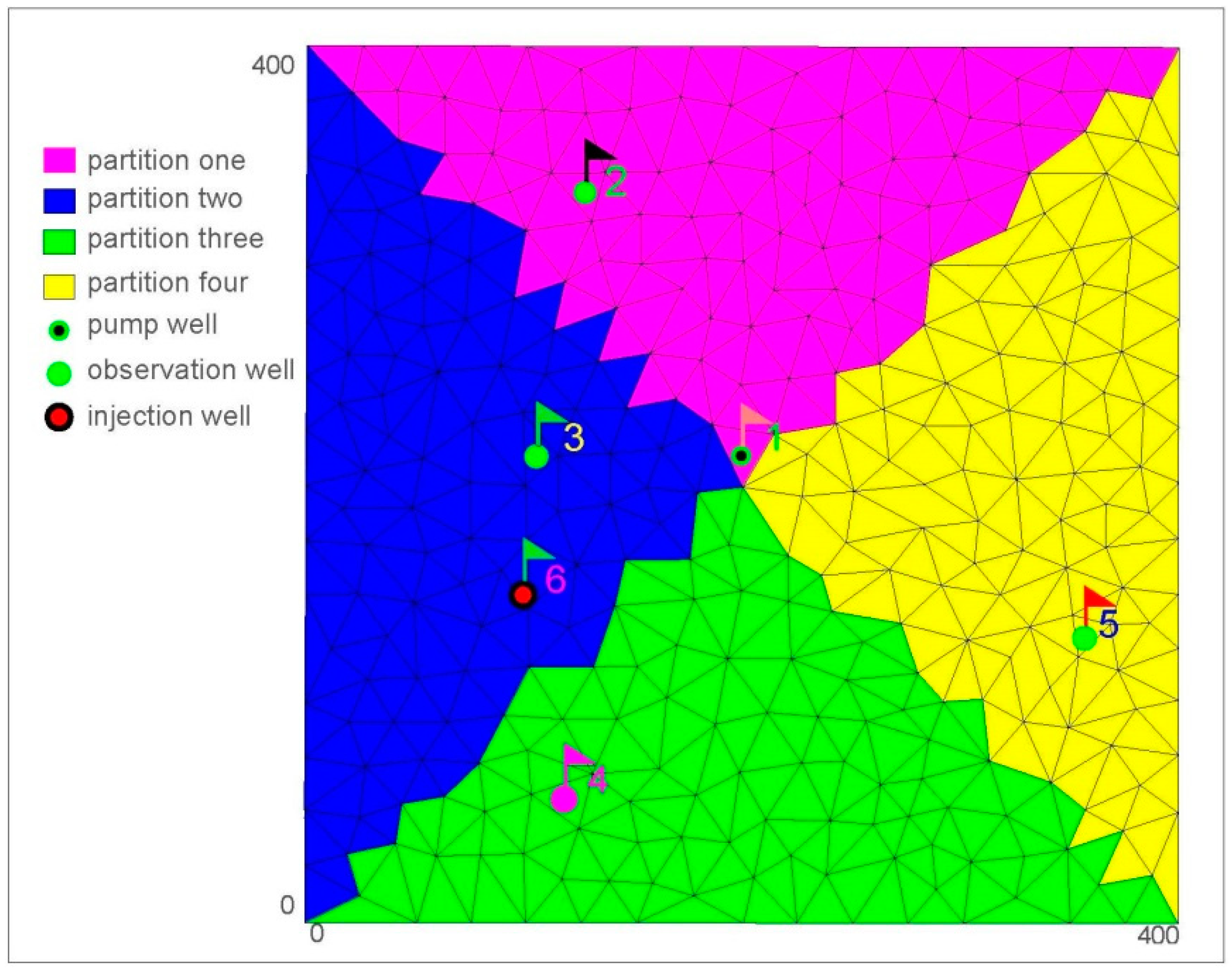
To verify the effectiveness of the method in solving the interval-based parametric groundwater head equation, we establish a synthetic two-dimensional confined aquifer flow model in this section. The confined aquifer has an extent of 400 m × 400 m in horizontal dimensions, and a thickness of 10 m. The total numbers of subdivision triangular elements are 620. Taking the aquifer base as the reference surface, the top elevation of the aquifer is 10 m. The initial water head of the aquifer is uniformly set at 100 m, the initial hydraulic gradient is zero, and the left boundary of the aquifer is defined as a constant-head boundary with a value of 100 m. The remaining three boundaries of the aquifer are set to be general-head boundaries (GHB) in which the head, the hydraulic conductivity and the reciprocal of the distance are 100 m, 1 m/day and 0.1 m⁻¹, respectively. The aquifer is heterogeneous and isotropic. According to different hydraulic conductivity values chosen at different regions, the aquifer is divided into four sections.

A graphic representation of the aquifer associated with a sample discretization used in the numerical simulation is shown in Figure 1. The values of the hydraulic conductivities of different zones are shown in

Table 1. Hydraulic conductivity in each zone of the model.

Partition	Hydraulic Conductivity (Average Value) (m/day)
One	1
Two	10
Three	5
Four	3

. From Figure 1, one can see that the pumping well (well No. 1 in Figure 1), which has coordinates of (200 m, 200 m), is located at the center of the aquifer. Meanwhile, each section contains an observation well. Considering steady-state flow, we will calculate and analyze three scenarios in the following sections. For Scenario One, the conductivities of the four sections are considered as the interval variable. On the basis of Scenario One, an injection well at coordinates of (100 m, 150 m) is added in Scenario Two. On the basis of Scenario Two, additional interval of boundary conditions is considered in Scenario Three. To verify the effectiveness of this proposed method, the degree of problem complexity increases from Scenario One to Scenario Three.

Where the numerical calculations are performed, we adopt the Groundwater Flow Model (GFModel) program which is based on an arbitrary polygon finite-difference method, developed by the first author (Guiming Dong) of China University of Mining and Technology [52]. The domain of interest is discretized into polygons. Further refinement of the discretization mesh does not provide noticeable improvement of the simulation results. Adopting the method of superposition of the osmotic matrix of the triangular element to form the coefficient matrix, the GFModel is a newly developed program, which can deal with the common boundary conditions, sources and sinks, and time-dependent hydrogeological parameters and can also carry out three-dimensional groundwater flow MC calculation, the general perturbation calculation, and interval parameter perturbation calculation.

4.1. Scenario One

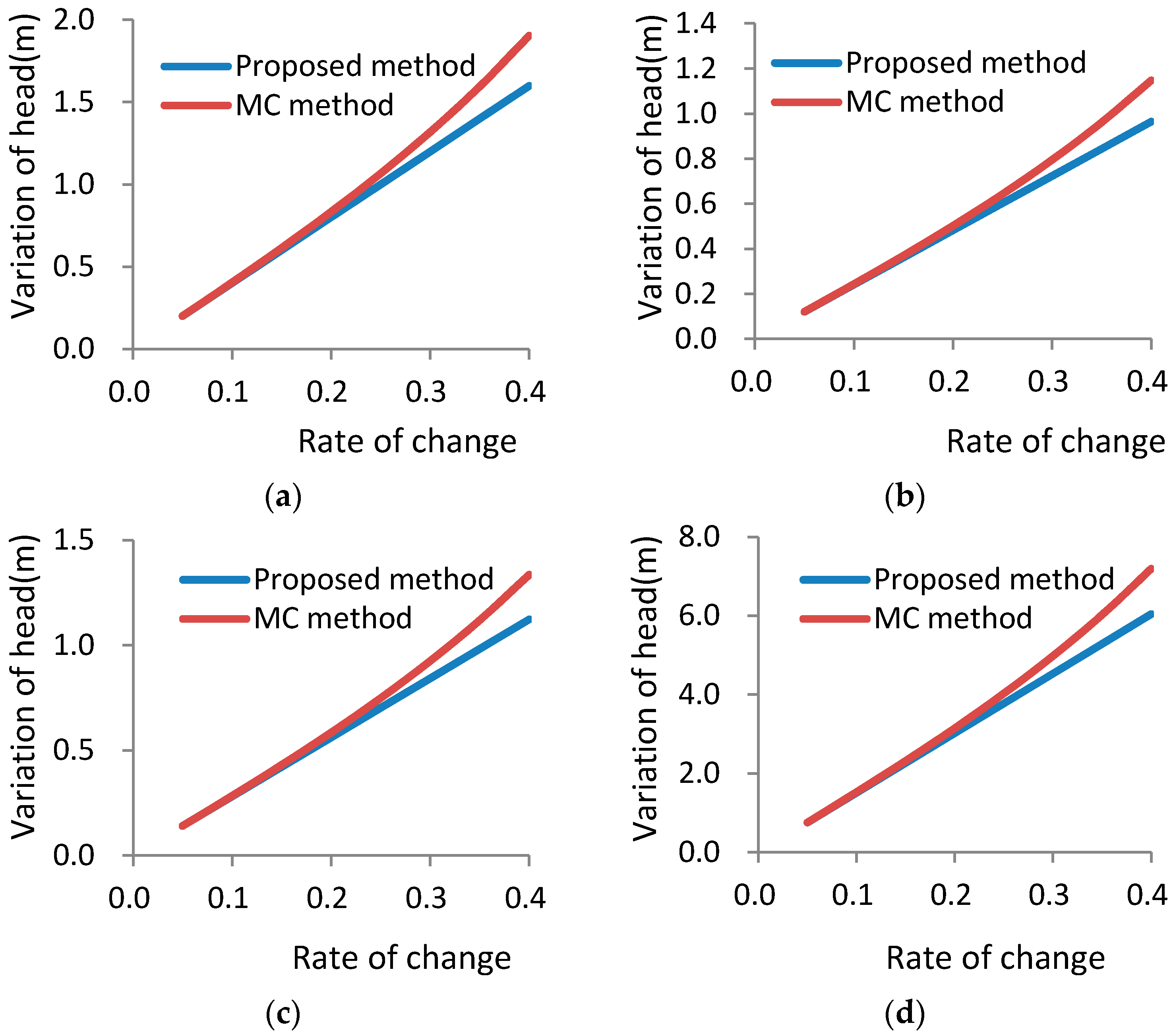
We set the flow of the pumping wells to be 1500 m³/day. Increasing at 0.05 intervals, the rate of change in the hydraulic conductivity changes from 0.05 to 0.4 in four zones seen in Figure 1, where the average value multiplied by the rate of change is equal to half of the variation of the parameter as referring to Equation (10). For example, the average hydraulic conductivity of the first partition is 1 m/day, when the rate of change is 0.2, then the interval of the hydraulic conductivity is [0.8, 1.2], and the variation of the parameter is 0.4 m/day. Moreover, we perform a comparative analysis of the MC method and the method proposed in this paper. The number of realizations used in the MC method is found to be 6.25 × 10⁶ after some numerical exercises. The maximum, minimum and variation of the groundwater head obtained by the MC method are taken as theoretical values. Using a computer with 4 GB of memory and CPU frequency of 2.5 GHz, the calculation time of MC is 2.6 days, and the calculation time of the IUM is 4.2 s. The results are shown in Figure 2,

Table 2. Calculation results table for Scenario One (unit: m).

Rate of Change	Observation Well No. 2
	MC Calculation Results			IUM Calculation Results			Relative Error (%)
	Lowest Head	Highest Head	Variations in Head	Lowest Head	Highest Head	Variations in Head
0.05	97.8684	98.0687	0.2003	97.8760	98.0758	0.1998	0.28
0.1	97.7515	98.1552	0.4037	97.7762	98.1757	0.3995	1.03
0.15	97.621	98.2342	0.6133	97.6763	98.2756	0.5993	2.28
0.2	97.4741	98.3067	0.8326	97.5764	98.3755	0.7991	4.02
0.25	97.3076	98.3733	1.0657	97.4765	98.4753	0.9988	6.27
0.3	97.1174	98.4348	1.3174	97.3766	98.5752	1.1986	9.02
0.35	96.8979	98.4917	1.5938	97.2767	98.6751	1.3984	12.27
0.4	96.6419	98.5447	1.9028	97.1769	98.7750	1.5981	16.01
Rate of Change	Observation Well No. 3
	MC Calculation Results			IUM Calculation Results			Relative Error (%)
	Lowest Head	Highest Head	Variations in Head	Lowest Head	Highest Head	Variations in Head
0.05	98.6456	98.7665	0.1209	98.6506	98.7711	0.1205	0.28
0.1	98.5751	98.8187	0.2436	98.5903	98.8314	0.2411	1.04
0.15	98.4963	98.8664	0.3701	98.5300	98.8916	0.3616	2.28
0.2	98.4078	98.9102	0.5024	98.4697	98.9519	0.4822	4.02
0.25	98.3074	98.9504	0.643	98.4095	99.0122	0.6027	6.26
0.3	98.1927	98.9876	0.7948	98.3492	99.0725	0.7233	9.01
0.35	98.0605	99.022	0.9615	98.2889	99.1327	0.8438	12.24
0.4	97.9062	99.054	1.1478	98.2287	99.1930	0.9643	15.98
Rate of Change	Observation Well No. 4
	MC Calculation Results			IUM Calculation Results			Relative Error (%)
	Lowest Head	Highest Head	Variations in Head	Lowest Head	Highest Head	Variations in Head
0.05	98.4301	98.5709	0.1408	98.4359	98.5763	0.1404	0.28
0.1	98.348	98.6318	0.2838	98.3657	98.6466	0.2809	1.04
0.15	98.2564	98.6874	0.4311	98.2955	98.7168	0.4213	2.27
0.2	98.1534	98.7385	0.5851	98.2253	98.7870	0.5617	4
0.25	98.0367	98.7854	0.7488	98.1551	98.8572	0.7021	6.23
0.3	97.9034	98.8288	0.9254	98.0848	98.9274	0.8426	8.95
0.35	97.7498	98.869	1.1193	98.0146	98.9976	0.983	12.18
0.4	97.5707	98.9064	1.3358	97.9444	99.0678	1.1234	15.9
Rate of Change	Observation Well No. 5
	MC Calculation Results			IUM Calculation Results			Relative Error(%)
	Lowest Head	Highest Head	Variations in Head	Lowest Head	Highest Head	Variations in Head
0.05	92.005	92.7623	0.7572	92.0305	92.7857	0.7552	0.27
0.1	91.5633	93.0893	1.526	91.6529	93.1633	1.5104	1.02
0.15	91.0697	93.3879	2.3182	91.2753	93.5409	2.2656	2.27
0.2	90.5145	93.6617	3.1472	90.8977	93.9185	3.0208	4.01
0.25	89.8852	93.9135	4.0283	90.5201	94.2961	3.776	6.26
0.3	89.1661	94.146	4.9799	90.1425	94.6737	4.5312	9.01
0.35	88.3364	94.3612	6.0249	89.7649	95.0513	5.2864	12.26
0.4	87.3684	94.5612	7.1928	89.3873	95.4289	6.0416	16

and

Table 3. Root mean square error (RMSE) calculation results of variations in head for Scenario One.

Rate of Change	0.05	0.1	0.15	0.2	0.25	0.3	0.35	0.4
RMSE	0.2236	0.3162	0.3873	0.4472	0.5000	0.5477	0.5916	0.6325

.

The smallest head and the largest head in each observation well decrease and increase respectively as the hydraulic conductivity rate of change increases, and the variations in head and the relative error increase correspondingly. The results of the proposed method show that when the rate of change is less than 0.2, the relative error of the head variation is generally limited to within 5%; while when the rate of change is less than 0.3, the relative error of the head variation is generally limited to within 10%, as seen in Table 1.

The theoretical head variation obtained from the MC method in the observation wells displays somewhat nonlinear relationship with the rate of change in the hydraulic conductivity. Instead, the relationship is best described as piecewise-linear. As can be seen from Figure 2, the theoretical head variation follows a nice linear relationship with the rate of change when the latter is less than 0.2. However, the theoretical variation starts to deviate from the linear trend when the rate of change is greater than 0.2.

For a given rate of change, when the hydraulic conductivities of four sections simultaneously take their minimum values, the head for the observation well is the same as the minimum theoretical head. Similarly, when the hydraulic conductivities of four sections simultaneously take their maximum values, the head for the observation well is also the same as the maximum theoretical head. The variations in the head calculated by the general perturbation method are the same as those calculated using the method proposed in this study. In the meantime, the corresponding values of ψ all must be positive in Equation (22), because only in this case, the general perturbation method calculated results will be the same with the computational result of Equation (25), which suggests that the general perturbation method has a close relationship with the proposed method.

4.2. Scenario Two

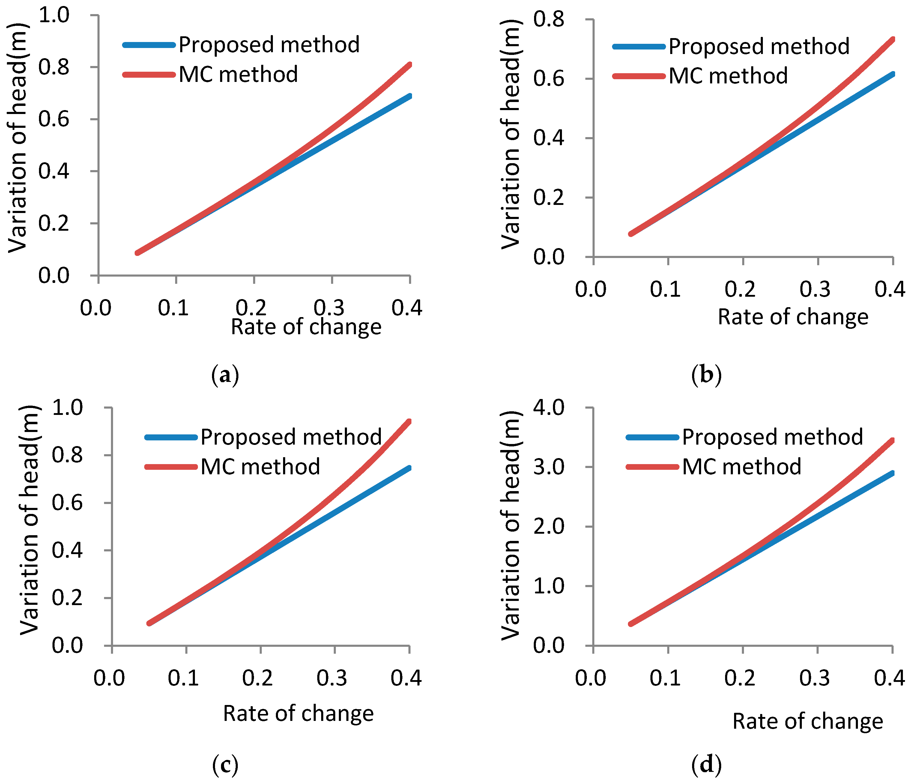
Based on Scenario One, we install a new injection well with a flow rate of 1500 m³/day at the coordinates (100 m, 150 m). The hydraulic conductivity rate of change is also adjusted from 0.05 to 0.4. The number of realizations used in the MC method model is also 6.25 × 10⁶. The calculation time of MC and the IUM is same as that on the scenario One. The results are shown in Figure 3,

Table 4. Calculation results table for Scenario Two (unit: m).

Rate of Change	Observation Well No. 2
	MC Calculation Results			IUM Calculation Results			Relative Error (%)
	Lowest Head	Highest Head	Variations in Head	Lowest Head	Highest Head	Variations in Head
0.05	99.1171	99.2035	0.0864	99.1157	99.2018	0.0861	0.27
0.1	99.067	99.2409	0.1739	99.0726	99.2449	0.1723	0.95
0.15	99.0114	99.2754	0.264	99.0296	99.2880	0.2584	2.12
0.2	98.9493	99.3071	0.3578	98.9865	99.3310	0.3445	3.72
0.25	98.8793	99.3364	0.457	98.9435	99.3741	0.4306	5.78
0.3	98.7997	99.3634	0.5637	98.9004	99.4172	0.5168	8.33
0.35	98.7082	99.3886	0.6804	98.8573	99.4602	0.6029	11.39
0.4	98.6018	99.412	0.8102	98.8143	99.5033	0.689	14.95
Rate of Change	Observation Well No. 3
	MC Calculation Results			IUM Calculation Results			Relative Error (%)
	Lowest Head	Highest Head	Variations in Head	Lowest Head	Highest Head	Variations in Head
0.05	99.1447	99.2219	0.0772	99.1440	99.2210	0.077	0.3
0.1	99.0996	99.2552	0.1556	99.1055	99.2595	0.154	1.05
0.15	99.0493	99.2857	0.2364	99.0671	99.2980	0.2309	2.3
0.2	98.9927	99.3136	0.3209	99.0286	99.3365	0.3079	4.05
0.25	98.9286	99.3393	0.4107	98.9901	99.3750	0.3849	6.29
0.3	98.8553	99.3631	0.5078	98.9516	99.4135	0.4619	9.04
0.35	98.7708	99.385	0.6143	98.9131	99.4519	0.5388	12.28
0.4	98.6722	99.4055	0.7333	98.8746	99.4904	0.6158	16.02
Rate of Change	Observation Well No. 4
	MC Calculation Results			IUM Calculation Results			Relative Error (%)
	Lowest Head	Highest Head	Variations in Head	Lowest Head	Highest Head	Variations in Head
0.05	100.4527	100.5463	0.0936	100.4468	100.5401	0.0933	0.32
0.1	100.4138	100.6029	0.1891	100.4001	100.5867	0.1866	1.32
0.15	100.379	100.6676	0.2885	100.3535	100.6334	0.2799	3.01
0.2	100.3479	100.7422	0.3943	100.3069	100.6800	0.3731	5.36
0.25	100.3199	100.8288	0.5088	100.2602	100.7266	0.4664	8.34
0.3	100.2947	100.9302	0.6355	100.2136	100.7733	0.5597	11.93
0.35	100.2718	101.0502	0.7783	100.1669	100.8199	0.653	16.1
0.4	100.2511	101.1935	0.9424	100.1203	100.8666	0.7463	20.81
Rate of Change	Observation Well No. 5
	MC Calculation Results			IUM Calculation Results			Relative Error (%)
	Lowest Head	Highest Head	Variations in Head	Lowest Head	Highest Head	Variations in Head
0.05	96.1732	96.5366	0.3634	96.1744	96.5368	0.3624	0.28
0.1	95.9612	96.6935	0.7322	95.9933	96.7180	0.7247	1.03
0.15	95.7243	96.8368	1.1125	95.8121	96.8992	1.0871	2.29
0.2	95.4578	96.9682	1.5104	95.6309	97.0803	1.4494	4.04
0.25	95.1557	97.089	1.9333	95.4497	97.2615	1.8118	6.29
0.3	94.8105	97.2006	2.3901	95.2686	97.4427	2.1741	9.04
0.35	94.4123	97.3038	2.8916	95.0874	97.6239	2.5365	12.28
0.4	93.9476	97.3998	3.4522	94.9062	97.8050	2.8988	16.03

and

Table 5. RMSE calculation results of variations in head for Scenario Two.

Rate of Change	0.05	0.1	0.15	0.2	0.25	0.3	0.35	0.4
RMSE	0.2236	0.3162	0.3873	0.4472	0.5000	0.5477	0.5916	0.6325

.

The results of Scenario Two are consistent with their counterparts in Scenario One, with some slight discrepancies in terms of specific values shown in Table 3 and Figure 3. For the same rate of change in the hydraulic conductivity, the relative errors of observation well 3 and observation well 5 are basically the same in both scenarios; while the relative error of observation well 4 in Scenario Two is slightly larger than its corresponding value in Scenario One. Moreover, the relative error of the observation well 2 under Scenario Two is slightly less than its corresponding value under Scenario One. It is obvious that although Scenario Two is more complicated hydrogeologically (as it involves an additional injection well) than that of Scenario One, the accuracy of the proposed method does not show any noticeable decline. In addition, the results of the proposed method show that when the rate of change is less than 0.2, the relative error of the head variation is generally less than 5%; while when the rate of change is less than 0.3, the relative error of the head variation is generally less than 10%.

For a given rate of change of the hydraulic conductivity, further analysis shows that when the hydraulic conductivities of four sections simultaneously take their minimum values, the head for the observation well does not correspond to the minimum theoretical head calculated from the MC method. Similar conclusion can be drawn when the hydraulic conductivities of four sections simultaneously take their maximum values. This finding is certainly quite different from that of Scenario One. Taking the observation well 4 as an example, with a rate of change of 0.2, when the hydraulic conductivities of four sections are set at their minimum and maximum values simultaneously, the heads of observation well 4 are 100.62 and 100.41 m, respectively. These values are clearly different from the minimum (100.35 m) and the maximum (100.74 m) heads calculated using the MC method.

Based on above analysis, one can conclude that the result of the general perturbation method will differ from the method proposed in this paper. That implies that the corresponding value of ψ in Equation (22) is not always positive. Using observation well 4 as an example, when the hydraulic conductivity rate of change is all 0.2 in four sections, the head variation of the observation well is 0.20 m using the general perturbation method, which is obviously different from the head variation of 0.37 m calculated using the method of this study. It also shows that the method proposed in this study can calculate the extreme values of the head at any given node, whereas the general perturbation method only calculates the head variation of the node under a certain variation, which is obviously different.

4.3. Scenario Three

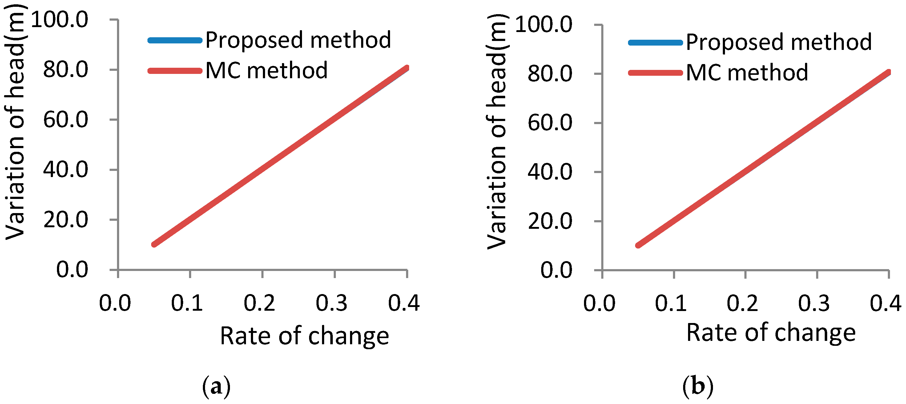
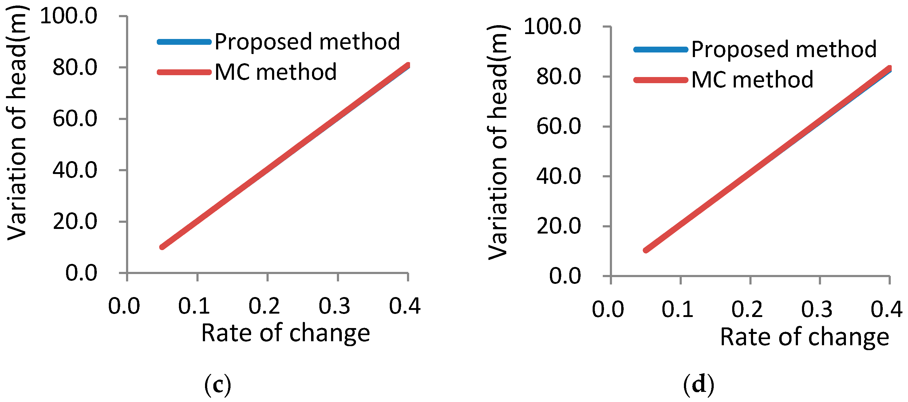
The difference between Scenario Three and Scenario Two is that the number of hydrogeological elements with interval variations, and the hydrogeological elements with interval variations, include the hydraulic conductivities of four sections, the head at the head boundary, the hydraulic conductivity, and the head at GHB. The reciprocal of the distance at GHB is constant. The hydraulic conductivity rate of change also changes from 0.05 to 0.4 in four sections. The numbers of realizations used in the MC method model are also 6.25 × 10⁶ times. The calculation time of MC is 4.1 days, while the calculation time of the IUM is only 4.2 s. The results are shown in Figure 4,

Table 6. Calculation results table for Scenario Three (unit: m).

Rate of Change	Observation Well No. 2
	MC Calculation Results			IUM Calculation Results			Relative Error (%)
	Lowest Head	Highest Head	Variations in Head	Lowest Head	Highest Head	Variations in Head
0.05	94.1189	104.2004	10.0815	94.1151	104.2025	10.0874	-0.06
0.1	89.068	109.2383	20.1703	89.0714	109.2462	20.1748	-0.02
0.15	84.0113	114.2732	30.2619	84.0277	114.2898	30.2621	0
0.2	78.948	119.3051	40.357	78.9840	119.3335	40.3495	0.02
0.25	73.8765	124.3347	50.4581	73.9403	124.3772	50.4369	0.04
0.3	68.7955	129.3619	60.5665	68.8966	129.4209	60.5243	0.07
0.35	63.7017	134.3872	70.6854	63.8530	134.4646	70.6116	0.1
0.4	58.5928	139.4107	80.8179	58.8093	139.5083	80.699	0.15
Rate of Change	Observation Well No. 3
	MC Calculation Results			IUM Calculation Results			Relative Error(%)
	Lowest Head	Highest Head	Variations in Head	Lowest Head	Highest Head	Variations in Head
0.05	94.1441	104.2213	10.0772	94.1418	104.2233	10.0815	-0.04
0.1	89.0965	109.2566	20.1601	89.1010	109.2640	20.163	-0.01
0.15	84.0431	114.2889	30.2458	84.0603	114.3048	30.2445	0
0.2	78.9832	119.3184	40.3351	79.0195	119.3455	40.326	0.02
0.25	73.9152	124.3456	50.4304	73.9788	124.3863	50.4075	0.05
0.3	68.8376	129.3707	60.5331	68.9380	129.4270	60.489	0.07
0.35	63.7481	134.3939	70.6458	63.8973	134.4678	70.5705	0.11
0.4	58.6436	139.4154	80.7719	58.8565	139.5085	80.652	0.15
Rate of Change	Observation Well No. 4
	MC Calculation Results			IUM Calculation Results			Relative Error (%)
	Lowest Head	Highest Head	Variations in Head	Lowest Head	Highest Head	Variations in Head
0.05	95.4547	105.5433	10.0886	95.4466	105.5402	10.0936	-0.05
0.1	90.4155	110.6001	20.1846	90.3998	110.5871	20.1873	-0.01
0.15	85.3804	115.6652	30.2848	85.3530	115.6339	30.2809	0.01
0.2	80.3488	120.7401	40.3913	80.3062	120.6807	40.3745	0.04
0.25	75.3202	125.8274	50.5071	75.2593	125.7275	50.4682	0.08
0.3	70.2943	130.9296	60.6353	70.2125	130.7743	60.5618	0.12
0.35	65.2703	136.0506	70.7803	65.1657	135.8211	70.6554	0.18
0.4	60.2483	141.1954	80.947	60.1189	140.8680	80.7491	0.24
Rate of Change	Observation Well No. 5
	MC Calculation Results			IUM calculation results			Relative Error(%)
	Lowest Head	Highest Head	Variations in Head	Lowest Head	Highest Head	Variations in Head
0.05	91.1783	101.5286	10.3503	91.1738	101.5374	10.3636	-0.13
0.1	85.9656	106.6861	20.7205	85.9920	106.7192	20.7272	-0.03
0.15	80.7276	111.8301	31.1025	80.8102	111.9010	31.0908	0.04
0.2	75.4604	116.9617	41.5013	75.6284	117.0828	41.4544	0.11
0.25	70.1571	122.0831	51.926	70.4466	122.2646	51.818	0.21
0.3	64.8106	127.1951	62.3845	65.2648	127.4464	62.1816	0.33
0.35	59.4111	132.2985	72.8874	60.0830	132.6282	72.5452	0.47
0.4	53.9448	137.3947	83.4499	54.9012	137.8100	82.9088	0.65

and

Table 7. RMSE calculation results of variations in head for Scenario Three.

Rate of Change	0.05	0.1	0.15	0.2	0.25	0.3	0.35	0.4
RMSE	0.2236	0.3162	0.3873	0.4472	0.5000	0.5477	0.5916	0.6325

.

The smallest head and the largest head for each observation well decrease and increase, respectively, as the hydraulic conductivity rate of change increases, and the variations in head and the relative error increase correspondingly. The results of the proposed method show that when the rate of change reaches 0.4, the maximum of the relative error is only 0.65%. This suggests that the relative error is generally limited to 1%.

There is a nice linear relationship between the theoretical head variation calculated from the MC method and the rate of change of the hydraulic conductivity, as can be seen from Figure 4. Interestingly enough, the head variation calculated by the proposed method of this study shows almost the same linear relationship with the rate of change in the hydraulic conductivity. This explains why the two methods have relatively small relative errors. It is obvious that, although the number of hydrogeological elements that are allowed to change in Scenario Three is larger (Scenario Three includes seven changing hydrogeological elements), the linearity of the system interval response is improved, and the accuracy of the method is improved as well. Therefore, the number of intervals does not appear to be the primary factor determining the accuracy of the proposed method. Because the degree of linearity of Scenario Three is higher than that of Scenario Two, it is reasonable to infer that the degree of linearity should be the main factor affecting the accuracy of the proposed method.

As in Scenario Two, the head for the observation well is not always the same as the minimum (or maximum) theoretical head when all the hydrogeological elements take their minimum (or maximum) values. The result of the general perturbation method is also different from that obtained from the method of this study. Once again, using observation well 4 as an example, with a rate of change of 0.1, where the rate of change is for all the seven changing hydrogeological elements, the head variation of the observation well is 19.90 m using the general perturbation method. This result is obviously different from the head variation of 20.19 m calculated by the method of this study. It can be seen from the three scenarios of numerical examples when three conditions, including the aquifer are confined aquifer, ${\phi }_i\left(\alpha \right)$ and ${\varphi }_i\left(\alpha \right)$ both are linear expressions and the interval of the changing elements is little change, are satisfied in the same time, the IUM can perform better, while any of the above three conditions are not satisfied, the IUM validity has not yet been checked. The inverse of matrix is the main factor that influences the calculation efficiency of the method. For the above problems, we will carry out research in the following study. In addition, the method can only obtain the changing interval of the head, while giving the statistical characteristics of the head.

5. Conclusions

In this study, in contrast to the stochastic methods used in many numerical simulations of groundwater flow and solute transport, a new concept involving interval mathematics is proposed to quantify the uncertainty analysis of groundwater flow and solute transport. This concept originates from the concept of interval uncertainty. The form of the interval-type groundwater flow governing equation is presented, and the interval parameter perturbation method is provided. Since this method only required matrix inversion to obtain the derivative of the head for the changing hydrogeological elements, the method is computationally much more efficient than the conventional MC method. Using this method, the interval response of the groundwater head can be obtained, which is different from the value obtained by the general perturbation method.

Three hypothetical scenarios with an increasing degree of hydrogeological complexity and uncertainty are used as examples to illustrate the performance of the proposed method, including its accuracy and robustness. It appears that the accuracy of the method depends on the linearity between the simulated head variation and the changing hydrogeological elements. In addressing practical problems, the proposed method is recommended when the rate of change for the changing hydrogeological elements is less than a certain value such as 0.2, as great linearity between the simulated head variation and the changing hydrogeological elements has been identified under such condition. Further research is needed to determine the upper limit of the rate of change for the changing hydrogeological elements when this method is used under a wide range of hydrogeological conditions.

References

- Xu, T.; Valocchi, A.J. A Bayesian approach to improved calibration and prediction of groundwater models with structural error. Water Resour. Res. 2015, 51, 9290–9311. [Google Scholar] [CrossRef]
- Tartakovsky, D.M. Assessment and management of risk in subsurface hydrology: A review and perspective. Adv. Water Resour. 2013, 51, 247–260. [Google Scholar] [CrossRef]
- Joodavi, A.; Zare, M.; Ziaei, A.N.; Ferre, T.P.A. Groundwater management under uncertainty using a stochastic multi-cell model. J. Hydrol. 2017, 551, 265–277. [Google Scholar] [CrossRef]
- Marchant, B.; Mackay, J.; Bloomfield, J. Quantifying uncertainty in predictions of groundwater levels using formal likelihood methods. J. Hydrol. 2016, 540, 699–711. [Google Scholar] [CrossRef]
- Rojas, R.; Kahunde, S.; Peeters, L.; Batelaan, O.; Feyen, L.; Dassargues, A. Application of a multimodel approach to account for conceptual model and scenario uncertainties in groundwater modelling. J. Hydrol. 2010, 394, 416–435. [Google Scholar] [CrossRef] [Green Version]
- Brink, C.V.D.; Zaadnoordijk, W.J.; Burgers, S.; Griffioen, J. Stochastic uncertainties and sensitivities of a regional-scale transport model of nitrate in groundwater. J. Hydrol. 2008, 361, 309–318. [Google Scholar] [CrossRef]
- Refsgaard, J.C.; Christensen, S.; Sonnenborg, T.O. Review of strategies for handling geological uncertainty in groundwater flow and transport modeling. Adv. Water Resour. 2012, 36, 36–50. [Google Scholar] [CrossRef]
- Nilsson, B.; Hojberg, A.L.; Refsgaard, J.C. Uncertainty in geological and hydrogeological data. Hydrol. Earth Syst. Sci. 2007, 11, 2675–2706. [Google Scholar] [CrossRef]
- Matott, L.S.; Babendreier, J.E.; Purucker, S.T. Evaluating uncertainty in integrated environmental models: A review of concepts and tools. Water Resour. Res. 2009, 45, 735–742. [Google Scholar] [CrossRef]
- Freeze, R.A. A stochastic-conceptual analysis of one-dimensional groundwater flow innonuniform homogeneous media. Water Resour. Res. 1975, 12, 567. [Google Scholar]
- Smith, L.; Freeze, R.A. Stochastic analysis of steady state groundwater flow in a bounded domain: 2. Two-dimensional simulations. Water Resour. Res. 1979, 15, 1543–1559. [Google Scholar] [CrossRef]
- James, A.L.; Oldenburg, C.M. Linear and Monte Carlo uncertainty analysis for subsurface contaminant transport simulation. Water Resour. Res. 1997, 33, 2495–2508. [Google Scholar] [CrossRef]
- Tonkin, M.; Doherty, J. Calibration-constrained Monte Carlo analysis of highly parameterized models using subspace techniques. Water Resour. Res. 2009, 45, 206–216. [Google Scholar] [CrossRef]
- Graham, W.; Mclaughlin, D. Stochastic analysis of nonstationary subsurface solute transport: 1. Unconditional moments. Water Resour. Res. 1989, 25, 2331–2355. [Google Scholar] [CrossRef]
- Zhang, D.; Winter, C.L.; Laboratory, N. Moment-Equation Approach to Single Phase Fluid Flow in Heterogeneous Reservoirs. SPE J. 1999, 4, 118–127. [Google Scholar]
- Lu, Z.; Zhang, D. On stochastic modeling of flow in multimodal heterogeneous formations. Water Resour. Res. 2002, 38, 8-1–8-15. [Google Scholar] [CrossRef]
- Winter, C.L.; Tartakovsky, D.M.; Guadagnini, A. Numerical solutions of moment equations for flow in heterogeneous composite aquifers. Water Resour. Res. 2002, 38, 13-1–13-8. [Google Scholar] [CrossRef]
- Winter, C.L.; Tartakovsky, D.M.; Guadagnini, A. Moment Differential Equations for Flow in Highly Heterogeneous Porous Media. Surv. Geophys. 2003, 24, 81–106. [Google Scholar] [CrossRef]
- Sagar, B. Galerkin Finite Element Procedure for analysing flow through random media. Water Resour. Res. 1978, 14, 1035–1044. [Google Scholar] [CrossRef]
- Dettinger, M.D.; Wilson, J.L. First order analysis of uncertainty in numerical models of groundwater flow part: 1. Mathematical development. Water Resour. Res. 1981, 17, 149–161. [Google Scholar] [CrossRef]
- Sitar, N.; Cawlfield, J.D.; Kiureghian, A.D. First-order reliability approach to stochastic analysis of subsurface flow and contaminant transport. Water Resour. Res. 1987, 23, 794–804. [Google Scholar] [CrossRef]
- Connell, L.D. An analysis of perturbation based methods for the treatment of parameter uncertainty in numerical groundwater models. Transp. Porous Media 1995, 21, 225–240. [Google Scholar] [CrossRef]
- Venue, M.L.; Andrews, R.W.; Ramarao, B.S. Groundwater travel time uncertainty analysis using sensitivity derivatives. Water Resour. Res. 1989, 25, 1551–1566. [Google Scholar] [CrossRef]
- Serrano, S.E. A new approach in modelling groundwater pollution under uncertainty. Probab. Eng. Mech. 1989, 4, 85–98. [Google Scholar] [CrossRef]
- Li, S.G.; Liao, H.S.; Ni, C.F. Stochastic modeling of complex nonstationary groundwater systems. Adv. Water Resour. 2004, 27, 1087–1104. [Google Scholar] [CrossRef]
- Ni, C.F.; Li, S.G. Modeling groundwater velocity uncertainty in nonstationary composite porous media. Adv. Water Resour. 2006, 29, 1866–1875. [Google Scholar] [CrossRef]
- Ni, C.F.; Li, S.G. Approximate Analytical Solution to Groundwater Velocity Variance in Unconfined Trending Aquifers in the Presence of Complex Sources and Sinks. J. Hydrol. Eng. 2009, 14, 1119–1125. [Google Scholar] [CrossRef]
- Beven, K.; Freer, J. Equifinality, data assimilation, and uncertainty estimation in mechanistic modelling of complex environmental systems using the GLUE methodology. J. Hydrol. 2001, 249, 11–29. [Google Scholar] [CrossRef]
- Vázquez, R.F.; Beven, K.; Feyen, J. GLUE Based Assessment on the Overall Predictions of a MIKE SHE Application. Water Resour. Manag. 2009, 23, 1325–1349. [Google Scholar] [CrossRef]
- Hastings, W.K. Monte Carlo Sampling Methods Using Markov Chains and Their Applications. Biometrika 1970, 57, 97–109. [Google Scholar] [CrossRef]
- Geman, S.; Geman, D. Stochastic Relaxation, Gibbs Distributions, and the Bayesian Restoration of Images. IEEE Trans. Pattern Anal. Mach. Intell. 1984, 6, 721–741. [Google Scholar] [CrossRef] [PubMed]
- Gelfand, A.E. Sampling-Based Approaches to Calculating Marginal Densities. J. Am. Stat. Assoc. 1990, 85, 398–409. [Google Scholar] [CrossRef]
- Gilks, W.R.; Best, N.G.; Tan, K.K.C. Adaptive Rejection Metropolis Sampling within Gibbs Sampling. J. R. Stat. Soc. 1995, 44, 455–472. [Google Scholar] [CrossRef]
- Haario, H.; Saksman, E.; Tamminen, J. An Adaptive Metropolis Algorithm. Bernoulli 2001, 7, 223–242. [Google Scholar] [CrossRef]
- Elsheikh, A.H.; Wheeler, M.F.; Hoteit, I. Nested sampling algorithm for subsurface flow model selection, uncertainty quantification, and nonlinear calibration. Water Resour. Res. 2013, 49, 8383–8399. [Google Scholar] [CrossRef]
- Elsheikh, A.H.; Demyanov, V.; Tavakoli, R.; Christie, M.A.; Wheeler, M.F. Calibration of channelized subsurface flow models using nested sampling and soft probabilities. Adv. Water Resour. 2015, 75, 14–30. [Google Scholar] [CrossRef]
- Yakirevich, A.; Pachepsky, Y.A.; Gish, T.J.; Guber, A.K.; Kuznetsov, M.Y.; Cady, R.E.; Nicholsone, T.J. Augmentation of groundwater monitoring networks using information theory and ensemble modeling with pedotransfer functions. J. Hydrol. 2013, 501, 13–24. [Google Scholar] [CrossRef]
- Zeng, X.K.; Ye, M.; Burkardt, J.; Wu, J.C.; Wang, D.; Zhu, X.B. Evaluating two sparse grid surrogates and two adaptation criteria for groundwater bayesian uncertainty quantification. J. Hydrol. 2016, 535, 120–134. [Google Scholar] [CrossRef]
- Huisman, J.A.; Rings, J.; Vrugt, J.A.; Sorg, J.; Vereecken, H. Hydraulic properties of a model dike from coupled bayesian and multi-criteria hydrogeophysical inversion. J. Hydrol. 2010, 380, 62–73. [Google Scholar] [CrossRef]
- Lu, D.; Ye, M.; Curtis, G.P. Maximum likelihood bayesian model averaging and its predictive analysis for groundwater reactive transport models. J. Hydrol. 2015, 529, 1859–1873. [Google Scholar] [CrossRef]
- Qiu, Z.; Elishakoff, I.; Starnes, J.H., Jr. The bound set of possible eigenvalues of structures with uncertain but non-random parameters. Chaos Solitons Fractals 1996, 7, 1845–1857. [Google Scholar] [CrossRef]
- Qiu, Z.; Ma, L.; Wang, X. Unified form for static displacement, dynamic response and natural frequency analysis based on convex models. Appl. Math. Model. 2009, 33, 3836–3847. [Google Scholar] [CrossRef]
- Qiu, Z.; Ni, Z. An inequality model for solving interval dynamic response of structures with uncertain-but-bounded parameters. Appl. Math. Model. 2010, 34, 2166–2177. [Google Scholar] [CrossRef]
- Muhanna, R.L.; Mullen, R.L. Bounds of Structural Response for All Possible Loading Combinations. J. Struct. Eng. 1999, 125, 98–106. [Google Scholar]
- Chen, L.; Shen, Z.Y.; Yang, X.H.; Liao, Q.; Yu, S.L. An interval-deviation approach for hydrology and water quality model evaluation within an uncertainty framework. J. Hydrol. 2014, 509, 207–214. [Google Scholar] [CrossRef]
- Yang, G.Q.; Guo, P.; Li, M.; Zhang, L.D. An improved solving approach forinterval-parameter programming and application to an optimal allocation ofirrigation water problem. Water Resour. Manag. 2016, 30, 701–729. [Google Scholar] [CrossRef]
- Li, M.; Fu, Q.; Singh, V.P.; Liu, D. An interval multi-objective programming model for irrigation water allocation under uncertainty. Agric. Water Manag. 2018, 196, 24–36. [Google Scholar] [CrossRef]
- Siddiqui, S.; Azarm, S.; Gabriel, S. A modified benders decomposition method for efficient robust optimization under interval uncertainty. Struct. Multidiscip. Optim. 2011, 44, 259–275. [Google Scholar] [CrossRef]
- Jiang, C.; Hana, X.; Liu, G.P. A nonlinear interval number programming method for uncertain optimization problems. Eur. J. Oper. Res. 2008, 188, 1–13. [Google Scholar] [CrossRef]
- Wu, H.C. The Karush–Kuhn–Tucker optimality conditions in an optimization problem with interval-valued objective function. Eur. J. Oper. Res. 2007, 176, 46–59. [Google Scholar] [CrossRef]
- Qiu, Z.P. Convex Method Based on Non-Probabilistic Set-Theory and Its Application; National Defence Industry Press: Beijing, China, 2005; pp. 59–79. (In Chinese) [Google Scholar]
- Li, P.T. Inversion of Hydrogeological Parameters Based on the Nested Bayesian Method. Master’s Thesis, China University of Mining and Technology, Xuzhou, China, 2016; pp. 23–38. (In Chinese). [Google Scholar]
Figure 1.
Division graph of ideal groundwater flow model and map showing the locations of the pumping well and the observation wells. (Pumping well: 1; observation wells: 2–5; injection well: 6; length unit: m.)
Figure 2.
Comparison of two methods in Scenario One ((a) observation well 2; (b) observation well 3; (c) observation well 4; (d) observation well 5).
Figure 3.
Comparison of the two methods in Scenario Two ((a) observation well 2; (b) observation well 3; (c) observation well 4; (d) observation well 5).
Figure 4.
Comparison of two methods in Scenario Three ((a) observation well 2; (b) observation well 3; (c) observation well 4; (d) observation well 5).