Quantifying the Effects of Near-Bed Concentration on the Sediment Flux after the Operation of the Three Gorges Dam, Yangtze River


Key Laboratory of Water Cycle and Related Land Surface Processes, Institute of Geographic Sciences and Natural Resources Research, Chinese Academy of Sciences, Beijing 100101, China
Water 2017, 9(12), 986; https://doi.org/10.3390/w9120986
Submission received: 12 November 2017
/
Revised: 11 December 2017
/
Accepted: 15 December 2017
/
Published: 18 December 2017
(This article belongs to the Special Issue Adaptive Catchment Management and Reservoir Operation)
Abstract
:The regime of sediment transport in the Jingjiang Reach has significantly changed from quasi-equilibrium to sub-saturation since the impoundment of the Three Gorges Dam (TGD), and vertical profiles of suspended sediment concentration (SSC) have changed accordingly. Vertical profiles of SSC data measured at three hydrological stations in the Jingjiang Reach (Zhicheng, Shaishi, and Jianli), before and after the impoundment of TGD, were collected and analyzed. Analytic results indicate a remarkably large concentration in the near-bed zone (within 10% of water depth from the river-bed) in a sub-saturated channel. The maximum measured concentration was up to 15 times the vertical average concentration, while the ratio in quasi-equilibrium channel was less than four times that. Concentrations normalized with reference concentration at the same height, and may decrease with increasing values of suspension index (settling velocity over shear velocity). In addition, concentration near the water surface may be larger than concentration in the near-bed region when the suspension index is smaller than 0.01. Sediment flux transported in the near-bed zone may be up to 35% of the total sediment flux in unsaturated flows. The relationship between deviations of estimating sediment flux when ignoring the near-bed concentration and discharge in flood season and non-flood season are different in unsaturated and quasi-equilibrium channels. Analysis indicates that, in the quasi-equilibrium channel, more attention should be paid to near-bed concentration during non-flood season, the same as measurements during flood season with larger discharge.
1. Introduction
The majority (>90%) of river-borne flux is closely associated with sediment [1]. A significant proportion of sediments are transported in suspension, as the bed load at river mouths is often less than 1% of the total solid transport [2].
Various vertical profiles of suspended sediment concentration (SSC) have been observed by field observation. For example, these profiles include linear type including linear or quasi-linear (with different gradients), parabolic curve, and mixed linear type [3,4]. For different linear types, the difference between concentration on the water surface and concentration near the bed varies. For linear type, the difference of concentration in the vertical direction increases with increasing slope, and the rate of variation in a vertical direction is constant. Furthermore, the linear types can be observed in estuaries with smaller concentrations [3]. For the parabolic type, the rate of variation in a vertical direction varies, and exists in a relatively larger concentration in the near-bed region. For the parabolic type, the concentration in the near-bed region is a kind of tailing phenomenon, and this kind of vertical profile can be observed in tide water [3]. Various theories, i.e., gravity, diffusion, mixing, energy dissipation, and stochastic models have been applied to simulate the vertical distribution of SSC [5,6]. And various efforts have been focused on the temporal and spatial variation of SSC by field survey, especially the near-surface and near-bed concentration [7,8]. Zuo et al. [3] pointed out that larger concentrations in the near-bed region may be caused by flocculate, saline water and tidal wave. Based on observation in the Jingjiang River Reach after Three Gorges Dam’s impoundment, vertical profiles of SSC in channels with a changed sediment regime have revealed a remarkably large concentration in the near-bed region [9]. This indicates that, a larger concentration in the near-bed region can also be observed in a reservoir down-channel [9]. Erosion downstream is a living topic coping with sediment trapping in reservoirs. Varied sediment transport regimes and sediment-related problems in the middle reach (Jingjiang Reach, China) have a profound morphological impact on the lower reach, that is, navigation, pollutant and deposition in channels and ports, water and sediment management in stem channels, social and economic problems and so on [10]. Various studies focus on the changed sediment regime and its influences on the channel downstream (i.e., [11,12,13]). However, the characteristics of the distinct larger near-bed concentration and its effects on the river reach have not been widely analyzed.
Thus, the study aims to analyze the changed vertical profiles of SSC with changed sediment regimes. Based on vertical profiles of concentration, detailed characteristics of the tailing phenomena are analyzed. Then, the effects of high concentration in the near-bed region on sediment flux are estimated. Finally, the vertical distribution of suspended sediment concentration and its effects after dam operation are compared with data before operation.
2. Materials and Methods
2.1. Study Area and Data
The Yangtze River (YR) is the largest and longest river in China, and the third largest river in the world. The length of the YR is approximately 6.3 × 10³ km, and the drainage area is approximately 1.8 × 10⁶ km2.
The Three Gorges Dam (TGD) is located at the exit of the upper YR, Yichang in Hubei province [14]. The dam is 185 m high and the storage capacity of the reservoir is 3.9 × 10⁸ m3. The main purposes of the project are flood control, power generation and navigation. It started to impound water in 2003. After 2003, bedload and suspended load from the upper drainage area of the YR are trapped in the reservoir of the TGD. For suspended sediment load (SSL), more than 70% may be trapped during the first 10 years of operation, and approximately half of the SSL may be trapped during the operation over 40–100 years; the ratio may decrease to 15% and 10% after 80 years and 100 years, respectively [15]. Therefore, the SSL entering the middle and lower channel decreases, which leads to erosion of river reach down the dam [16]. During the operation of the TGD, the downstream channel erosion was extensive, and riverbed incision was accelerated [17].
The Jingjiang River is the river reach between Zhicheng and Chenglingji stations, with another two controlling stations of Shashi and Jianli (Figure 1). The length of the Jingjiang River Reach is approximately 348 km, and it is 64 km downstream from the TGD. The length of the upper and the lower part of the Jingjiang River Reach are approximately 172 km and 176 km, respectively [18,19]. During the operation of the TGD, the flow regime and sediment regime of the Jingjiang River Reach have changed [14].
Data measured at these three gauges in the Jingjiang Reach before and after the operation of TGD are collected (Table 1). Observed data are the vertical profiles of concentrations, discharges, wetted area, water depth, temperature, water stages, velocities and corresponding gradations. Data are measured by the Jingjiang Hydrology and Water Resources Surveying Bureau (JHWRSB), and published by the Yangtze River Water Resources Commission (YRWRC).
Vertical profiles measured before and after 2010 are different. For data measured before dam operation, there are only five measuring points in each vertical line. Typical vertical profiles of data measured before dam operation may be described with relative heights (y/H) of 0.94, 0.8, 0.6, 0.2, and 0.04 (data measured 24 September 2002, at Zhicheng station with distance left of 700 m), where y is the distance of each measured point from the riverbed (m), and H is the averaged water depth (m) of this vertical line. This means that the near-bed region (less than 10% depth) has one measuring point.
For data measured after dam operation, there are seven points in each vertical profile, with typical relative heights (y/H) of 0.98, 0.8, 0.4, 0.2, 0.1, 0.0307, 0.0061 (data measured 11 July 2011, at Jianli station with distance left of 1170 m). The two near-bed points are measured with distance of 0.5 m and 0.1 m from the bed, respectively.
2.2. Equations to Estimate the Effects of Near-Bed Concentration on Sediment Flux
The sediment load by the two near-bed points are compared with the total sediment load of the local vertical profile,
where Qsv(7) and Qsv(5) are vertical sediment flux by seven points and upper five points, respectively.
The result of ignoring these two points can also be estimated. The deviation ratio of sediment transport rate by omitting the two near-bed points can be calculated by forms as:
where Qs(7) and Qs(5) are sediment flux by seven points and five points, respectively. Qs(5) is estimated with two measured near-bed points being omitted artificially. For the cross-sectional estimation, there are only several vertical profiles. The delta-shaped area between the left bank and the first vertical line from the left bank is also considered. The delta-shaped area between the right bank and the last vertical line from the left bank is not considered due to the difficulty of identifying the right bank.
The specific values of data measured during pre- and post-operation may vary in different vertical lines, but the differences are limited. These vertical profiles measured before dam operation missed the near-bed region due to what has been done after operation. They are interpolated and extended to the near-bed region, with minimum relative height (y/H) of 0.006.
3. Results
3.1. Distinct Non-Uniform Vertical Distribution
3.1.1. Comparing with Vertical-Averaged Concentration
In order to describe the vertical profiles of SSC, the vertical profiles are compared with vertical-averaged concentration. The relative height of the vertical coordinate is expressed as y/H, in which y is the distance of each measured point from the riverbed (m), and H is the averaged water depth (m) of this vertical line. The relative concentration in the horizontal coordinate is expressed as Si/Savg, where Si is the measured concentration of the vertical profile (kg/m3), and Savg represents the vertical averaged concentration (kg/m3). The minimum distance of measuring points from the riverbed can be named as the reference height, and the corresponding concentration is the reference concentration.
Figure 2 compares the vertical distribution of sediment concentrations in the Jingjiang Reach before and after the TGD impounded water in 2003. Figure 2 shows that, after the dam operation, measured vertical profiles of suspended sediment at these two gauges show a distinctly high concentration in the near-bed zone.
For data measured after operation, the minimum relative height of measured points from the riverbed (y/H) is approximately 0.0051. The maximum relative concentrations (Si/Savg) are approximately 14.45 (Jianli) and 15.05 (Shashi). This kind of distinctly high concentration in the near-bed zone can be named as “tailing phenomena”. It indicates that more sediment is transported in areas near the riverbed; the measured two near-bed points make it much worse. According to the data, average concentrations of these two near-bed points may account for up to 1.86 times of vertical averaged concentration at Shashi hydrological station, and 2.73 times at Jianli hydrological station.
For data measured before operation, the minimum relative height of measured points from the riverbed (y/H) is approximately 0.014 (0.3 m from the riverbed). The maximum relative concentrations (Si/Savg) are approximately 3.62 (Jianli) and 2.30 (Shashi). The maximum relative concentrations (Si/Savg) for Zhicheng station is approximately 2.76. For Zhicheng station, there are no data measured after the dam operation. Thus, data measured at Zhicheng are not included in Figure 2. Data measured before dam operation can be viewed as short-tail tailing phenomena.
Relatively high concentrations near the bed region have also been pronounced. Relatively larger near-bed concentrations can also be observed in the estuary of Yangtze River, Qiantangjiang River and Taizhou sea area [20,21]. Figure 3 illustrates relative concentrations (Si/Savg) measured at several regions, which also demonstrated a kind of tailing phenomena. Relative concentration (Si/Savg) is estimated with measured concentration over vertical averaged concentration, as in Figure 2. Data measured at Yangtze Estuary are drawn from Zhang [20], data measured at Wuhan and Jiujiang River Reach are drawn from Tang et al. [22], and data at Oujiangkou and Taizhou sea areas are drawn from Dong et al. [21]. The maximum relative concentration (Si/Savg) is approximately 4.3, and the minimum relative height of measured points from the riverbed (y/H) is approximately 0.03. Therefore, this kind of vertical profile can be viewed as short-tail tailing phenomena. The tailing phenomena which is much apparent in the Middle Jingjiang River Reach can be viewed as long-tail tailing phenomena. The near-bed concentration of the S-type vertical distribution is also relatively larger [23]. The tailing phenomena in the estuary area can be observed during tide periods and non-flood seasons [20].
3.1.2. Comparing with Near-Bed Point
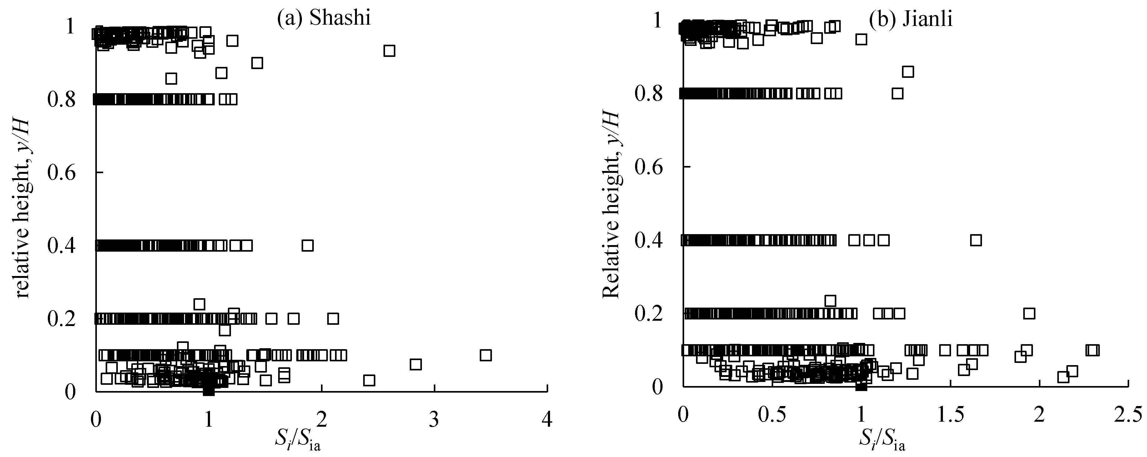
In order to highlight the concentration near the bed, the vertical profiles of suspended sediment load are compared with concentration of the near-bed point. The horizontal coordinate is Si/Sia, where Sia represents the measured concentration of the near-bed point (kg/m3). Only data measured after the operation are analyzed.
According to Si/Sia, the concentration near the bed is not absolutely larger than that of upper points, as shown in Figure 4. Vertical profiles can be grouped into two kinds: the first one is profiles in which concentration of the near-bed point is the largest (Type I), and the second one is profiles in which maximum concentration occurred in the near-bed region (Type II). All the vertical profiles observed in Zhang [20], Tang et al. [22], and Dong et al. [21] can be grouped as Type I with short-tail.
Figure 4 illustrates the vertical profiles measured after dam operation at Shashi and Jianli stations. For data measured after operation, approximately 27% of vertical profiles can be grouped as Type II (Jianli), and the ratio for Shashi station is approximately 48% (Table 2). The suspension index (ω/u*) in Table 2 is estimated with settling velocity (ω) over shear velocity (u*). According to Table 2, vertical profiles of Type I have a relatively larger chance of occurring in flood season, while vertical profiles of Type II have a relatively larger chance of occurring in non-flood season.
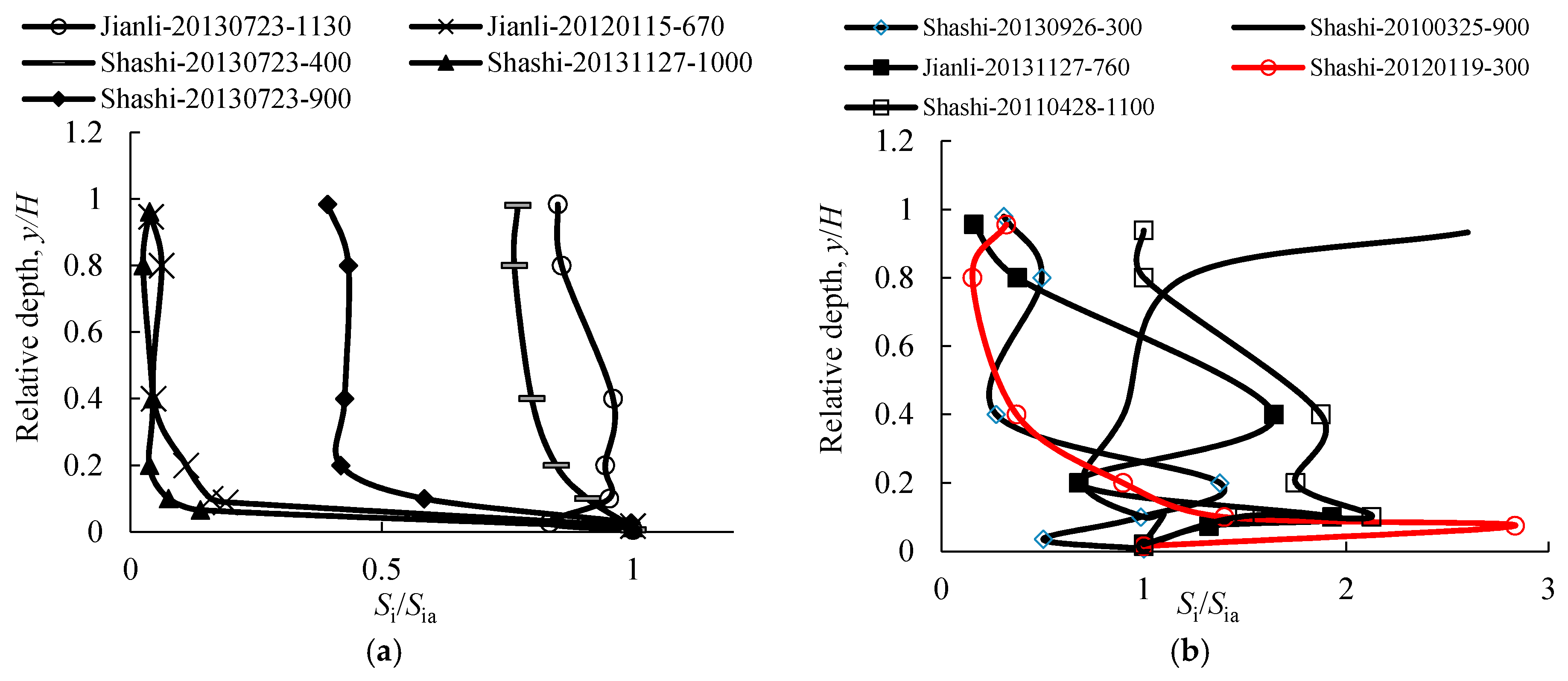
For Type I, five typical profiles are shown in Figure 5a, and five typical profiles of Type II are shown in Figure 5b. This shows that the concentrations of the near-bed region of Type I vary with different coefficients (ω/u*). For type II, the vertical distribution of concentration is much more complex, while concentration with relative height less than 0.04 is relatively large.
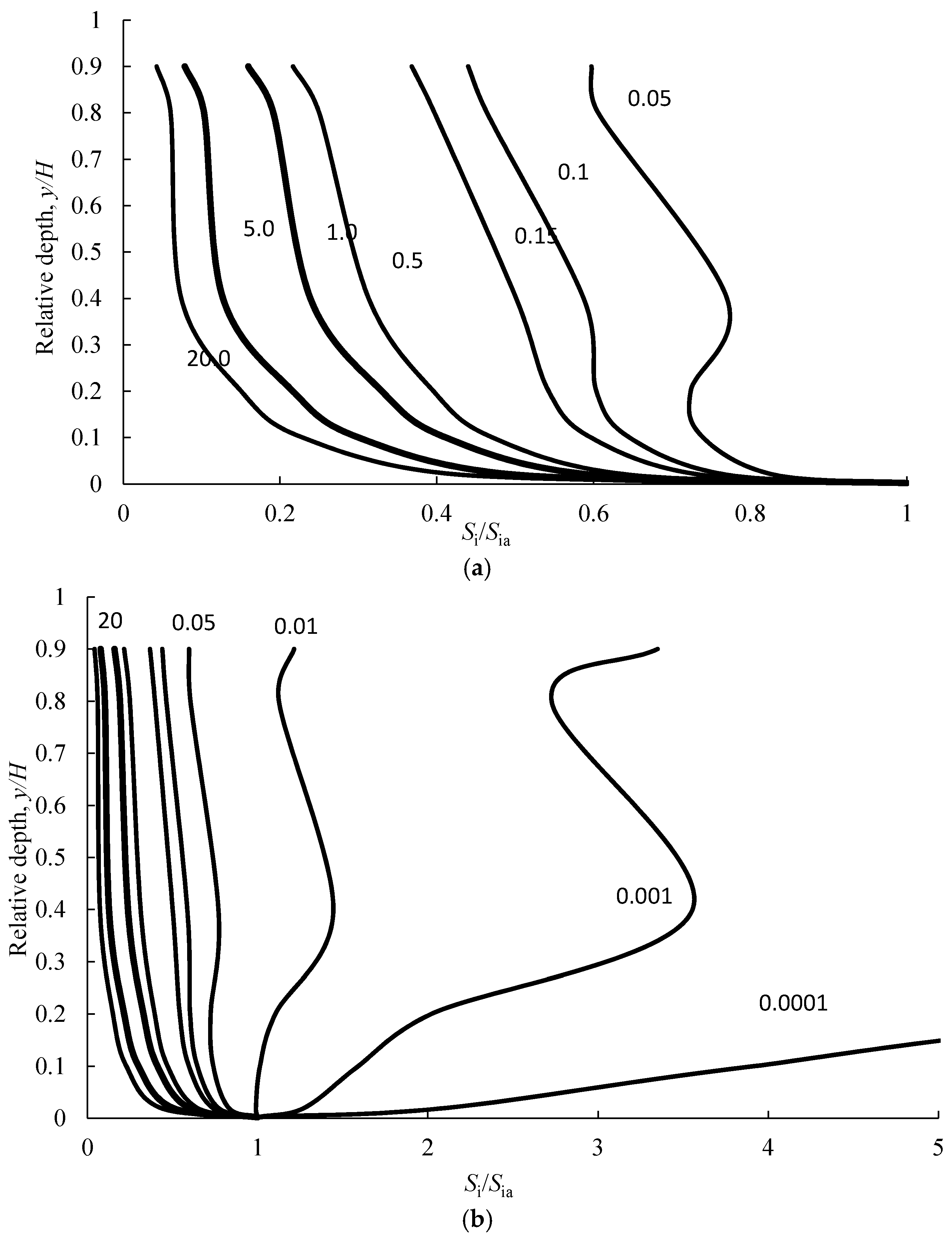
Figure 6 illustrates the vertical distribution of Si/Sia with different (ω/u*). In order to make it more readable, the coefficient in Figure 6 is (ω/u*). It shows that, the concentration of Si/Sia at the same relative height decreases with increasing coefficients (Figure 6a). When the coefficient decreases to less than 0.01, vertical profiles of Type I change to Type II (Figure 6b). One thing that should be pointed out is that lines in Figure 6 are estimated with data measured in flood seasons with Type I at Shashi station. The lines may vary with different data adopted, but the rules are the same: the concentration of Si/Sia at the same relative height (y/H) decreases with increasing coefficient (ω/u*), and Type I may change to Type II with a coefficient less than 0.01.
3.2. Effects on Sediment Flux
Suspended sediment transport is the most significant factor influencing estuaries in emorpho-dynamics, yet it is often one of the largest unknowns. As to sediment trapped by the TGD and changed sediment regime, the vertical distribution of suspended sediment varies in the Jingjiang River. The estimation of sediment flux of the Jingjiang River may also be influenced, which is important to navigation, channel management of the whole river system, and so on.
The tailing phenomena means that, sediment concentration within 10% of water depth from the river-bed cannot be ignored, otherwise it may lead to different results when estimating erosion or deposition by sediment-transport balance methods and volume methods. Thus, the effects of remarkably larger concentration in the near-bed region are analyzed.
3.2.1. Vertical Sediment Flux
In Figure 7, the Bi is the lateral distance of measured vertical lines from the left bank, and Bavg is the maximum width of the cross section. The maximum width of the cross section is assumed to be the maximum lateral distance from the left bank, namely the distance of the last vertical profiles from the left bank. It shows that these two kinds of vertical profiles may occur in the whole lateral cross section. The maximum R0 value is larger than 47%. The average ratios for these two, type profiles at Shashi station are 18% (Type I) and 13% (Type II). The average ratios for these two, type profiles at Jianli station are 22% (Type I) and 18% (Type II). Table 3 indicates that the R0-values for non-flood season are relatively larger than those of flood season.
Zhang [20] also pointed out that the near-bed concentration may affect the estimated sediment load when A = ω/(βku*) > 0.15, where ω is the settling velocity of uniformed particles, k is the Karmen coefficient, u* is the shear velocity of approaching flow, and β is a coefficient for non-uniform sediment. When suspension index A = ω/(βku*) equals two, suspended sediment may concentrate in an area with a distance of 0.2 times the water depth from the riverbed, and the ratio of near-bed transportation over the total transportation (R) is approximately 30% [20]. Tang et al. [22] pointed out that, the near-bed concentration may be more apparent when ω/(ku*) > 5. The values of ω/u* are 0.06, 0.8 and 2 (with k = 0.4 and β = 1) by Zhang [20] and Tang et al. [22], respectively. For data illustrated in Figure 8, the values of ω/u* range from 0.001 to 0.201. Zhang [20] also pointed out that the tailing phenomena is more apparent with larger values of relative particle size (Di/Dm, particle-size over averaged particle size) of non-uniform sediment. The ratio (R) is approximately 25% when Di/Dm > 3 [20].
In total, initiation of motion, suspension threshold, and the vertical distribution of sand concentration in the water column all need to be determined for an accurate estimate of sediment transport.
3.2.2. Sectional Sediment Flux
Due to the larger contribution ratio of the two near-bed points (R0) in Figure 7, the contributions on sectional sediment flux can also be estimated. Figure 9 shows that, if the two near-bed points are not included, the sediment flux may be underestimated by approximately 40%. During flood season, the R-value may increase with increasing discharge, while the largest R-value may occur by measures in non-flood season. In total, the larger average R-value for flood season at Shashi station may be caused by larger discharge (Table 4).
This described situation may result in the different erosion amounts by sediment-transport balance method and volume method [25]. Yuan et al. [26] showed that, the contribution ratio by the near-bed concentration varies by different hydrological years and river reach. For a certain hydrological station, the contribution ratios may also vary with the inflow condition. Therefore, the impact of high concentration near the bed surface must be given more attention in the future, especially during non-flood season and flood season with larger discharge.
The influence of near-bed concentration on estimating the annual deposition by the sediment-balance method has also been analyzed by various studies [26,27]. Based on hydrology data and geometry data measured between 2002 and 2008, contributions of factors that may cause differences were distinguished. For the Yichang–Zhicheng River Reach, there are three kinds of factors that may contribute to deposition estimation with sediment-balance method, namely, sand dredging in the channel, the near-bed concentration, and non-balanced water runoff. For the Zhicheng–Shashi River Reach and Shashi–Jianli River Reach, there are four kinds of contributing factors, namely, sand dredging in the channel, the near-bed concentration, non-balanced water runoff, and simplified measurement.
Figure 10 illustrates the contribution ratios of different factors. The two ratios in Figure 10 are the contribution ratio by near-bed concentration over the total influencing factors, and contribution ratio by total influencing factors on the total deposition estimation. It shows that, for estimating the deposition with sediment-balance method, the contribution by near-bed concentration cannot be ignored, with ratios of 12%, 9% and 18%, respectively. As to its large magnitude of total deposition, the net deposition caused by near-bed concentration is 1.267 × 10⁷ m3, 9.80 × 10⁹ m3 and 2.303 × 10⁷ m3, respectively.
Dam construction has primarily contributed to sediment zonation (with different patterns of size distribution) weakening in the Jingjiang reaches (from Yichang to Chenglingji) over the last half-century [28]. The percentage of finer grouped particles (diameter less than 0.01 mm) decreased from 60% (2002) to approximately 40% (2008), and the medium sediment diameter increased from 0.052 mm (2002) to 0.081 mm (2008) [29]. The operation of the TGD and the ensuing decline of SSC was the main reason for the coarsening of the bed sediment in 1977–2003, especially at Shashi station (located 173 km downstream from Yichang station) [28]. It indicates that the coarser particulates had settled in the reservoir, and the river channel between Yichang and Shashi stations was badly eroded by clean water from the reservoir [28]. The coarser eroded sediment gradually settled along the channel between Shashi and Hankou stations due to the decrease in slope and current [28].
4. Discussion
Based on data measured after dam operation, the vertical profiles of SSC in the starved channel show a distinct tailing phenomena. Furthermore, it also influences the estimation of sediment flux. Data measured before dam operation are also collected to make a comparison, between both the vertical distribution and effects on sediment flux estimation.
4.1. Comparing with Data Measured Before Dam Operation
4.1.1. Vertical Profiles of SSC
Tailing phenomena can also be pronounced, however, the tailing phenomena is much more limited (relative concentration of 3.6 for Jianli and 2.3 for Shashi, as shown in Figure 5), the same as verticals by Zhang [20], Tang et al. [22], and Dong et al. [21]. Thus, vertical profiles before operation can be termed as short-tailing.
For data measured before operation, more data are measured in flood season. Approximately 20% (Jianli, Shashi, and Zhicheng stations) of vertical profiles can be grouped as Type II. In total, the occurring frequency of Type II increased after the operation of the TGD, especially at Shashi station (Table 5). In addition, the value of (ω/u*) increases dramatically.
Based on theoretical analysis, Zhang and Tan [30] stated that, if the concentration of coarser particles (eight times the finer particles) is larger than 33.5 kg/m3, the vertical distribution of concentration for finer particles may be different from that of the distribution of uniform particles, with dSf/dy > 0 (Figure 11). It also stated that this kind of distribution of particles finer than 0.01 mm can be observed in Tongguan and Huayuankou stations, Yellow River.
Figure 12 and Figure 13 illustrate the coarseness of suspended sediment and bed load before and after dam operation. For Shashi station, the percentage of particles coarser than 0.008 mm increases after the dam operation (Figure 12). For Jianli station, the percentage of particles coarser than 0.062 mm increases after the dam operation (Figure 12). The coarsening of bed materials after operation is apparent, especially at Shashi station (Figure 13). The coarsened suspended sediment and bed materials lead to the occurrence of remarkably large concentration in the near-bed region.
4.1.2. Sediment Flux
The interpolation made for data measured before dam operation has extended five point profiles to seven point profiles (with almost the same relative height of data after operation). Then, the deviations of flux estimation can also be calculated during the cross-sectional estimation. The maximum ratio may be nearly 35% (Figure 14). The maximum R-values may have occurred during non-flood season, and more attention should be paid on measuring during non-flood season (Table 6). The variances of R-value before and after dam operation are almost the same. However, the R-values during flood season may remain constant with increasing discharge for data measured before operation.
During the estimation of sectional averaged sediment flux, there is an assumption that may lead to uncertainties of estimation. For data measured before operation, the extension and interpolation may also lead to uncertainties. This kind of discrepancy can be verified by comparison between estimated and measured sectional discharge and concentration, as shown in Figure 15.
4.2. Contribution of Large Floods
The characteristics of suspended sediment concentration and yield at the event scale have been widely analyzed in various environments worldwide [31,32,33]. Floods are relevant for most of the suspended sediment load [34]. While sediment transport by floods correlated with flood regime, different flood regimes lead to different sediment transportation. For instance, analysis of a typical agro-catchment of the Loess Plateau shows that, the contribution of accumulative total sediment yield by the different flood regimes to the summed sediment yield of all of the examined 158 events are 4%, 13%, 6%, 21%, and 56% for Regimes A to E, respectively [35]. Thus, the flood regimes are analyzed and shown in Figure 16.
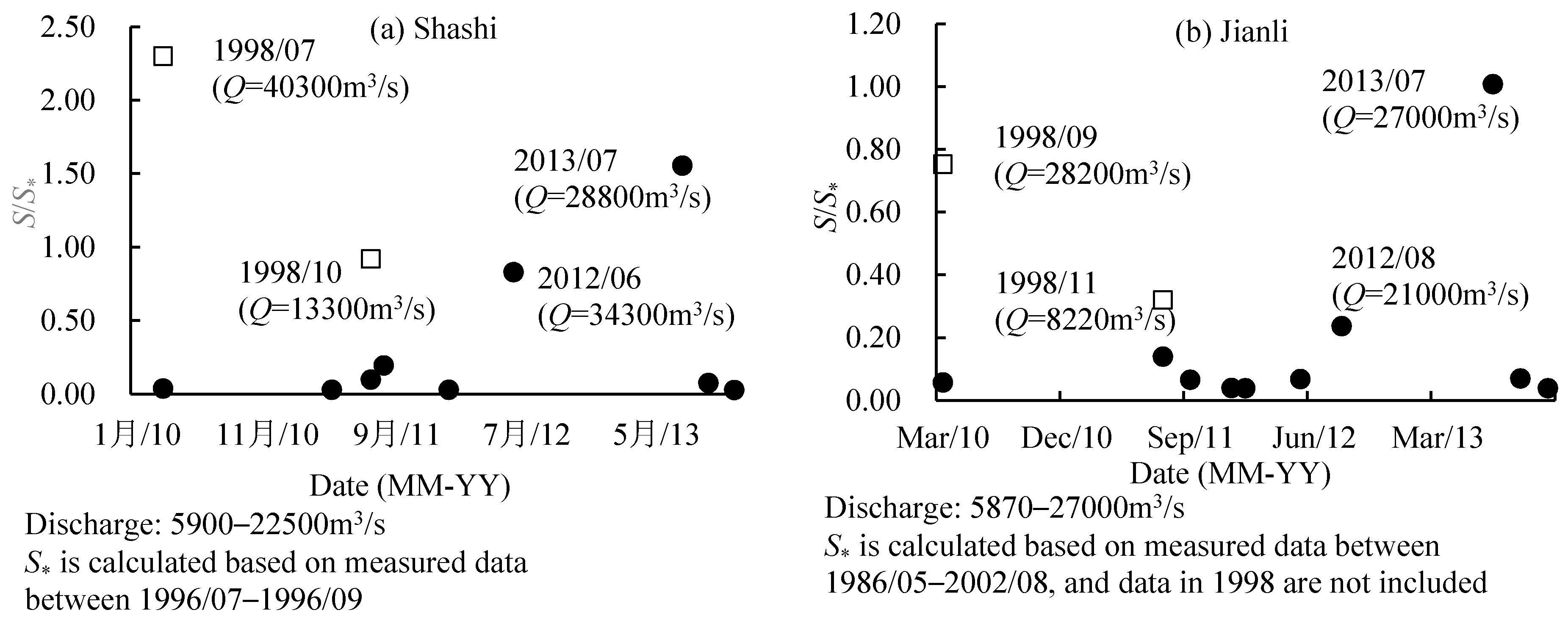
Measured data during flood period, such as the floods in 1998, 2013 and 2012, show an over-saturated state, and after the peak flood, the regime may change to pre-equilibrium or starved (Figure 16, Table 7). Figure 16 shows that, the relationships between discharge and concentration measured in floods with high discharges are different from those of floods with low discharges.
Shifts in the discharge-rating curves after three extreme flood events have also been observed by Whitaker et al. [36]. This indicates that the Jingjiang Reach of the YR has changed its sediment regime from pre-equilibrium to starved of sediment because of the operation of the TGD, and the flood regime may be different from the normal sediment regime. Shifts in the discharge-rating curves caused a period of channel instability [36]. Higher suspended sediment concentration may reduce the channel capacity and lead to channel erosion [37]. Finally, the fluvial erosion intensity during flood seasons is highly correlated with a corresponding incoming sediment coefficient [19].
The 1998 flood is the largest flood in the YR’s history since China’s economy entered the high-speed development period at the beginning of the 1980s, and it caused severe damage to the basin, causing losses exceeding 2 × 10¹⁰ RMB (Chinese currency) [38]. The higher water levels also led to overbank flows in the middle Yangtze River [39]. The sediment flux during this flood has been estimated [40]. The water stage in the 1998 flood was higher than that in the 1954 flood, despite the smaller total discharge during the 1998 flood.
The variability in the relationship between sediment concentration and water discharge (namely hysteretic patterns) has been used to explain the variability of sediment sources from one flood to another [42]. Whitaker et al. [36] compared the estimated sediment yield for an unsampled flood event, a single-event surrogate SSC–Q rating curve, and a long-term SSC–Q rating curve. Analysis revealed that, the long-term SSC–Q rating curve is estimated to be approximately 37% greater than the single-event SSC–Q estimates, which indicates a high degree of uncertainty. Analysis shows a high variability in the rating curve between similar floods [36]. Thus, large floods may also contribute to the occurrence of remarkably large concentration in the near-bed region (Type I), and the deviation of estimated sediment flux with sediment-balance method.
4.3. Connection with Dongting Lake
Reservoir sedimentation would disrupt previous flow and sediment delivery systems [43], especially channels down the dam. The TGD is the world’s biggest dam built on the largest river in China, the YR [14]. With impoundment of the TGD, channel reach downstream of the reservoir has adjusted to a changed flow and sediment situation, especially in the Jingjiang reach [29,44].
The Dongting Lake is connected with the Jingjiang River Reach with three distributaries’ channels and one outlet. It receives water from the main stream of the Yangtze River via three distributaries’ channels, and it discharges into the main stream of the Yangtze River at Chenglingji (the outlet of Dongting lake, Hunan Province, China). The annual runoff received from the Yangtze River is approximately 92.3 km3 through the Sankou distributary channels [45]. Li et al. [46] pointed out that, the channel changes serve as the primary factor in facilitating the decrease in the discharge diversion ratio, but not the main factor for the decreased amount of the discharge diversion. The occurring frequency of Type II increases after the operation of the TGD, especially at Shashi station, while two of the three distributary channels (Songzikou, Jingzhou City, Hubei Province, China and Taipingkou, Jingzhou City, Hubei Province, China) are located in the reach of upper Shashi station. Thus, vertical profiles of Type II may contribute to this relationship with much concentration transported into the lake.
4.4. Uncertainties
Turbidity monitoring is developed and applied attempting to better predict the continuous variability of suspended sediment concentration during a flood event, and in turn the total sediment yield [47,48]. The accurate in situ quantification of suspended sediment concentration is essential for model calibration and to identify sediment pathways and sediment flux [49].
The two near-bed points are measured with distances of 0.5 m and 0.1 m from the bed, respectively. As to the near-bed measuring, the small distance from the riverbed may be doubtful, as it is difficult to distinguish the riverbed. Equipment used in the field survey includes real-time kinematic Global Navigation Satellite System (RTK–GNSS), Total Station, vessel-mounted Acoustic Doppler Current Profilers (ADCP), Digital Level, Laser Particle Size Analyzer (LPSA), and so on. All the equipment and criteria have been strictly handled and executed by professional surveyors in JHWRSB. Several standards from the technical manual by JHWRSB [25] are listed in Table 8.
The main advantage of a RTK–GNSS survey is that it is faster, cheaper and easier to use during the surveying phase than classical topographic surveying [50]. Pagliari et al. [50] compared the differences between coordinates of the ground-controlled points estimated using RTK–GNSS, and those computed from the classical topographic measurements, during processing photogrammetric block. It pointed out that a RTK–GNSS survey may be sufficient to determine the requested tolerance [50]. Thus, in recent years, miniaturized components (GNSS receivers) have been adopted in field surveys [51].
ADCP is relatively easy to use, enables gathering various data types at once, can be attached to a RC platform, and has rapid three-dimensional flow structure measuring [52,53]. However, disadvantages of ADCP include snap-shot measurement of flow-change to errors, being time-consuming over large areas, and not being able to measure flow or depth in depths under 0.2 m [53]. As it is rather expensive, ADCP is relatively adopted to measure flow structure, flow discharge, bathymetry, bed load discharge, suspended load and channel change in field surveys [53]. Zhang et al. [54] pointed out that the error of ADCP in measuring cross-sections in the middle and lower YR channel is ±1% and the random uncertainty is 2–5%, and the integrated system (GPS and ASCP) delivered positioning with <15 cm accuracy vertically and <30 cm horizontally.
For sediment grain-size analysis, the results from LPSA and sieving are comparable when particles have a spherical shape [55]. Using a sieving method for coarser particles is more acceptable than for finer ones [55]. A sieving method is used in field surveys by JHWRSB [25]. According to the backscatter intensity of ADCP beams, suspended sediment concentration can also be estimated with inversion [56].
A major focus of research has been the development and application of turbidity monitoring, in an attempt to better predict the continuous variability of suspended sediment concentration during a flood event, and in turn the total sediment yield [47]. The concentration by sampling can be validated by echo intensity of the ADCP for future analysis.
5. Conclusions
The sediment regime of the Jingjiang Reach of the Yangtze River has changed dramatically because of the operation of the TGD. Based on vertical distribution data at the three controlling stations (Zhicheng, Shashi, and Jianli) on the Jingjiang Reach, the characteristics of remarkably large concentration in near-bed region and its implications are analyzed in this study. Our conclusions can be summarized as:
- (1)
- In sub-saturated channels, vertical distribution of suspended sediment concentration (SSC) is characterized by a remarkably large concentration in the near-bed zone (within 10% of water depth from the river-bed). The maximum measured concentration may be up to 15 times of vertical average concentration, while the ratio in quasi-equilibrium channels is less than four.
- (2)
- Concentrations normalized with reference concentration at the same height may decrease with increasing values of suspension index (ω/u*). Additionally, concentration near water surface may be larger than concentration in near-bed region when suspension index is smaller than 0.01.
- (3)
- After the dam operation, ignoring the near-bed concentration may cause up to 35% deviation when applied to estimate the sediment flux in the unsaturated flows. Deviations may increase with increasing discharge in flood season, while the maximum value may occur in non-flood season. Deviations in quasi-equilibrium channel may not increase with increasing discharge in flood season, while the maximum value may also occur in non-flood season. Deviations may increase with increasing particle size and suspension index.
Analytic results indicate that, in sub-saturated channels, more attention should be paid to near-bed concentration during non-flood season, the same as measurements during flood season with larger discharge.
Acknowledgments
This work was supported by the National Program on Key Basic Research Project (No. 2016YFC0402303); and the National Natural Science Foundation of China (Nos. 51579230, 51109198). We wish to express our deep gratitude to the Jingjiang Hydrology and Water Resources Surveying Bureau, Yangtze River Water Resources Commission for permission to access the hydrological data.
Conflicts of Interest
The author declares no conflict of interest.
References
- Ludwig, W.; AmiotteSuchet, P.; Probst, J.L. River discharge of carbon to the world’s oceans: Determining local inputs of alkalinity and of dissolved and particulate organic carbon. Comptes Rendus de L Academie des Sciences Serie II Fascicule A-Sciences de la Terre et des Planetes 1996, 323, 1007–1014. [Google Scholar]
- Asselman, N.E.M. Fitting and interpretation of sediment rating curves. J. Hydrol. 2000, 234, 228–248. [Google Scholar] [CrossRef]
- Zuo, S.H.; Li, J.F.; Wan, X.N.; Shen, H.T.; Fu, G. Characteristics of temporal and spatial variation of suspended sediment concentration in the Changjiang Estuary. J. Sediment Res. 2006, 3, 68–75, (In Chinese with English Abstract). [Google Scholar]
- Pal, D.; Ghoshal, K. Hydrodynamic interaction in suspended sediment distribution of open channel turbulent flow. Appl. Math. Modell. 2017, 49, 630–646. [Google Scholar] [CrossRef]
- Higgins, A.; Restrepo, J.C.; Otero, L.J.; Ortiz, J.C.; Conde, M. Vertical distribution of suspended sediment in the mouth area of the Magdalena River, Colombia. Lat. Am. J. Aquat. Res. 2017, 45, 724–736. [Google Scholar] [CrossRef]
- Nir, S.Q.; Sun, H.G.; Zhang, Y.; Chen, D.; Chen, W.; Chen, L.; Schaefer, S. Vertical distribution of suspended sediment under steady flows: Existing theories and fractional derivative model. Discret. Dyn. Nat. Soc. 2017, 2017, 1–11. [Google Scholar]
- Sahin, C.; Verney, R.; Sheremet, A.; Voulgaris, G. Acoustic backscatter by suspended cohesive sediment: Field observations, Seine Estuary, France. Cont. Shelf Res. 2017, 134, 39–51. [Google Scholar] [CrossRef]
- Armijos, E.; Crave, A.; Espinoza, R.; Fraizy, P.; Dos Santos, A.L.M.R.; Sampaio, F.; De Oliveria, E.; Santini, W.; Martinez, J.M.; Autin, P.; et al. Measuring and modelling vertical gradients in suspended sediments in the Solimões/Amazon River. Hydrol. Process. 2017, 31, 654–667. [Google Scholar] [CrossRef]
- He, L.; Chen, D.; Duan, G.L.; Zhu, Z.H.; Zhang, S.Y. Sediment suspension in the “starving” Jingjiang reach, downstream from the Three Gorges Dam, China. In Proceedings of the World Environmental and Water Resources Congress, West Palm Beach, FL, USA, 22–26 May 2016; pp. 303–313. [Google Scholar]
- Fang, H.Y.; Cai, Q.G.; Chen, H.; Li, Q.Y. Temporal changes in suspended sediment transport in a gullied loess basin: The lower Chabagou Creek on the Loess Plateau in China. Earth Surf. Process. Landf. 2008, 33, 1977–1992. [Google Scholar] [CrossRef]
- Zhang, R.; Zhang, S.H.; Xu, W.; Wang, B.D.; Wang, H. Flow regime of the three outlets on the south bank of Jingjiang River, China: An impact assessment of the Three Gorges Reservoir for 2003–2010. Stoch. Environ. Res. Risk Assess. 2015, 29, 2047–2060. [Google Scholar] [CrossRef]
- Fan, P.; Li, J.C.; Liu, Q.Q.; Singh, V.P. Case Study: Influence of morphological changes on flooding in Jingjiang River. J. Hydraul. Eng. 2008, 134, 1757–1766. [Google Scholar] [CrossRef]
- Yang, C.; Cai, X.B.; Wang, X.L.; Yan, R.R.; Zhang, T.; Zhang, Q.; Lu, X.R. Remotely sensed trajectory analysis of channel migration in lower Jingjiang Reach during the period of 1983–2013. Remote Sens. 2015, 7, 16241–16256. [Google Scholar] [CrossRef]
- Gao, B.; Yang, D.W.; Yang, H.B. Impact of the three Gorges Dam on flow regime in the middle and lower Yangtze River. Quat. Int. 2013, 304, 43–50. [Google Scholar] [CrossRef]
- Yang, H.; Tang, R. Study on the Evolution of Jingjiang Reach of Middle Yangtze River; China Water Power Press: Beijing, China, 1999. (In Chinese) [Google Scholar]
- Dai, Z.J.; Fagherazzi, S.; Mei, X.F.; Gao, J.J. Decline in suspended sediment concentration delivered by the Changjiang (Yangtze) River into the East China Sea between 1956 and 2013. Geomorphology 2016, 268, 123–132. [Google Scholar] [CrossRef]
- Xu, K.H.; Milliman, J.D. Seasonal variations of sediment discharge from the Yangtze River before and after impoundment of the Three Gorges Dam. Geomorphology 2009, 104, 276–283. [Google Scholar] [CrossRef]
- Xia, J.Q.; Zong, Q.L.; Deng, S.S.; Xu, Q.X.; Lu, J.Y. Seasonal variations in composite riverbank stability in the Lower Jingjiang Reach, China. J. Hydrol. 2014, 519, 3664–3673. [Google Scholar] [CrossRef]
- Xia, J.Q.; Zong, Q.L.; Zhang, Y.; Xu, Q.X.; Li, X.J. Prediction of recent bank retreat processes at typical sections in the Jingjiang Reach. Sci. China 2014, 57, 1490–1499. [Google Scholar] [CrossRef]
- Zhang, C.F. Vertical Profile of Non-Uniform Suspended Sediment Concentration in Yangtze Estuary. Master’s Thesis, Zhejiang University, Hangzhou, China, 2016. (In Chinese with English Abstract). [Google Scholar]
- Dong, X.T.; Li, R.J.; Fu, G.C.; Zhang, H.C. Relationship between vertical distribution of velocity and sediment concentration of sediment-laden flow. J. Hohai Univ. Natl. Sci. 2015, 43, 371–376, (In Chinese with English Abstract). [Google Scholar]
- Tang, M.L.; Cao, H.Q.; Li, Q.Y.; Zhai, W.L. Vertical distribution of suspended sediment in middle reaches of Yangtze River. Yangtze River 2017, 48, 6–11, (In Chinese with English Abstract). [Google Scholar]
- Feng, Q.; Xiao, Q.L. A new S-type vertical distribution of suspended sediment concentration. J. Sediment Res. 2015, 1, 19–24, (In Chinese with English Abstract). [Google Scholar]
- Xia, Y.F.; Xu, H.; Chen, Z.; Wu, D.W.; Zhang, S.Z. Experimental study on suspended sediment concentration and its vertical distribution under spilling breaking wave actions in silty coast. China Ocean Eng. 2011, 25, 565–575. [Google Scholar] [CrossRef]
- JHWRSB (Jingjiang Hydrology & Water Resources Surveying Bureau, Hydrology Bureau). Technical Report: Observation of Unbalanced Sediment Transport in the Lower Reaches of the Three Gorges Reservoir; Changjiang Water Resources Commission: Wuhan, Hubei, China, 2016. (In Chinese) [Google Scholar]
- Yuan, Y.; Zhang, X.F.; Duan, G.L. Modifying the channel erosion and deposition amount of Yichang-Jianli reach calculated by sediment discharge method. J. Hydroelectr. Eng. 2014, 33, 163–169, (In Chinese with English Abstract). [Google Scholar]
- Duan, G.L.; Peng, Y.B.; Guo, M.J. Comparative analysis on riverbed erosion and deposition amount calculated by different methods. J. Yangtze River Sci. Res. Inst. 2014, 31, 108–118, (In Chinese with English Abstract). [Google Scholar]
- Dai, S.B.; Lu, X.X. Sediment load change in the Yangtze River (Changjiang): A review. Geomorphology 2014, 215, 60–70. [Google Scholar] [CrossRef]
- Zhao, G.S.; Lu, J.Y.; Visser, P.J. Fluvial river regime in disturbed river systems: A case study of evolution of the Middle Yangtze River in post-TGD (Three Gorges Dam), China. J. Geol. Geophys. 2015, 4, 6. [Google Scholar] [CrossRef]
- Zhang, X.F.; Tan, G.M. Characteristics of vertical concentration distribution of non-uniform particles. J. Hydraul. Eng. 1992, 10, 48–52, (In Chinese with English Abstract). [Google Scholar]
- Lenzi, M.A.; Mao, L.; Comiti, F. Interannual variation of suspended sediment load and sediment yield in an alpine catchment. Hydrol. Sci. J. 2003, 48, 899–915. [Google Scholar] [CrossRef]
- Zabaleta, A.; Martinez, M.; Uriarte, J.A.; Antiguedad, I. Factors controlling suspended sediment yield during runoff events in small headwater catchments of the Basque Country. Catena 2007, 71, 179–190. [Google Scholar] [CrossRef]
- Langlois, J.L.; Johnson, D.W.; Mehuys, G.R. Suspended sediment dynamics associated with snowmelt runoff in a small mountain stream of Lake Tahoe (Nevada). Hydrol. Process. 2005, 19, 3569–3580. [Google Scholar] [CrossRef]
- Tena, T.; Batalla, R.J.; Vericat, D. Reach-scale suspended sediment balance downstream from dams in a large Mediterranean River. Hydrol. Sci. J. 2012, 57, 831–849. [Google Scholar] [CrossRef]
- Zhang, W.; Yuan, J.; Han, J.Q.; Huang, C.T.; Li, M. Impact of the Three Gorges Dam on sediment deposition and erosion in the middle Yangtze River: A case study of the Shashi Reach. Hydrol. Res. 2016, 175–186. [Google Scholar] [CrossRef]
- Whitaker, A.C.; Sato, H.; Sugiyama, H. Changing suspended sediment dynamics due to extreme flood events in a small pluvial-nival system in northern Japan. In Sediment Dynamics in Changing Environments; IAHS-AISH Publication: Christchurch, New Zealand, 2008; Volume 325, pp. 192–199. [Google Scholar]
- Li, L.Q.; Lu, X.X.; Chen, Z.Y. River channel change during the last 50 years in the middle Yangtze River, the Jianli reach. Geomorphology 2007, 85, 185–196. [Google Scholar] [CrossRef]
- Zhu, Y.H.; Fan, B.L.; Yao, S.M.; Sun, G.Z.; Li, F.Z. Propagation features of the 1998 big floods in the Jinagjiang Reach of the Yangtze River. In Advances in Water Resources and Hydraulic Engineering; Springer: Berlin/Heidelberg, Germany, 2009; pp. 1032–1037. [Google Scholar]
- Zong, Y.Q.; Chen, X.Q. The 1998 flood on the Yangtze, China. Nat. Hazards 2000, 22, 165–184. [Google Scholar] [CrossRef]
- Xu, K.Q.; Chen, Z.Y.; Zhao, Y.W.; Wang, Z.H.; Zhang, J.Q.; Hayashi, S.J.; Murakami, S.; Watanabe, M. Simulated sediment flux during 1998 big-flood of the Yangtze (Changjiang) River, China. J. Hydrol. 2005, 313, 221–223. [Google Scholar] [CrossRef]
- Zhou, W.H.; Chen, Y.H. The 1998 flood of the Yangtze River. Int. J. Sediment Res. 1999, 14, 61–66. [Google Scholar]
- Seeger, M.; Errea, M.-P.; Begueria, S.; Arnaez, J.; Marti, C.; Garcia-Ruiz, J.M. Catchment soil moisture and rainfall characteristics as determinant factors for discharge/suspended sediment hysteretic loops in a small headwater catchment in the Spanish Pyrenees. J. Hydrol. 2004, 288, 299–311. [Google Scholar] [CrossRef] [Green Version]
- Ran, L.; Lu, X.; Xin, Z.; Yang, X. Cumulative sediment trapping by reservoirs in large river basins: A case study of the Yellow River basin. Glob. Planet. Chang. 2013, 100, 308–319. [Google Scholar] [CrossRef]
- Xia, J.Q.; Deng, S.S.; Lu, J.Y.; Xu, Q.X.; Zong, Q.L.; Tan, G.M. Dynamic channel adjustments in the Jingjiang reach of the middle Yangtze River. Sci. Rep. 2016, 6, 22802. [Google Scholar] [CrossRef] [PubMed]
- Dou, H.; Jiang, J. Dongting Lake; Press of University of Science and Technology of China: Hefei, China, 2000. [Google Scholar]
- Li, N.; Wang, L.C.; Zeng, C.F.; Wang, D.; Liu, D.F.; Wu, X.T. Variations of runoff and sediment load in the Middle and Lower Reaches of the Yangtze River, China (1950–2013). PLoS ONE 2016, 11, e160154. [Google Scholar] [CrossRef] [PubMed]
- Orwin, J.F.; Smart, C.C. An inexpensive turbidimeter for monitoring suspended sediment. Geomorphology 2005, 68, 3–15. [Google Scholar] [CrossRef]
- Pfannkuche, J.; Schmidt, A. Determination of suspended particulate matter concentration from turbidity measurements: Particle size effects and calibration procedures. Hydrol. Process. 2003, 17, 1951–1963. [Google Scholar] [CrossRef]
- Stutter, M.; Dawson, J.J.C.; Glendell, M.; Napier, F.; Potts, J.M.; Sample, J.; Vinten, A.; Watson, H. Evaluating the use of in-situ turbidity measurements to quantify fluvial sediment and phosphorus concentration and flux in agricultural streams. Sci. Total Environ. 2017, 607–608, 391–402. [Google Scholar] [CrossRef] [PubMed]
- Pagliari, D.; Rossi, L.; Passoni, D.; Pinto, L.; De Michele, C.; Avanzi, F. Measuring the volume of flushed sediments in a reservoir using multi-temporal images acquired with UAS. Geomat. Nat. Hazards Risk 2017, 8, 150–166. [Google Scholar] [CrossRef]
- Bandini, F.; Jakobsen, J.; Olesen, D.; Reyna-Gutierrez, J.A.; Bauer-Gottwein, P. Measuring water level in rivers and lakes from lightweight unmanned aerial vehicles. J. Hydrol. 2017, 548, 237–250. [Google Scholar] [CrossRef]
- Togneri, M.; Lewis, M.; Neill, S.; Masters, I. Comparison of ADCP observations and 3D model simulations of turbulence at a tidal energy site. Renew. Energy 2017, 114, 273–282. [Google Scholar] [CrossRef]
- Kasvi, E.; Hooke, J.; Kurkela, M.; Vaaja, M.T.; Virtanen, J.P.; Hyyppa, H.; Alho, P. Modern empirical and modelling study approaches in fluvial geomorphology to elucidate sub-bend-scale meander dynamics. Prog. Phys. Geogr. 2017, 41, 533–569. [Google Scholar] [CrossRef]
- Zhang, Q.; Shi, Y.F.; Xiong, M. Geometric properties of river cross sections and associated hydrodynamic implications in Wuhan-Jiujiang river reach, the Yangtze River. J. Geogr. Sci. 2009, 19, 58–66. [Google Scholar] [CrossRef]
- Li, W.K.; Wu, Y.X.; Huang, Z.M.; Fan, R.; Lv, J.F. Measurement results comparison between Laser Particle Analyzer and Sieving method in particle size distribution. Zhongguo Fenti Jishu 2007, 5, 10–13, (In Chinese with English Abstract). [Google Scholar]
- Jin, W.F.; Liang, C.J.; Zhou, B.F.; Li, J.D. Measurement and analysis of high suspended sediment concentration in Jintang channel with vessel-mounted ADCP. J. Mar. Sci. 2009, 27, 31–39, (In Chinese with English Abstract). [Google Scholar]
Figure 1.
Sketch of the Yangtze River and Jingjiang River Reach.
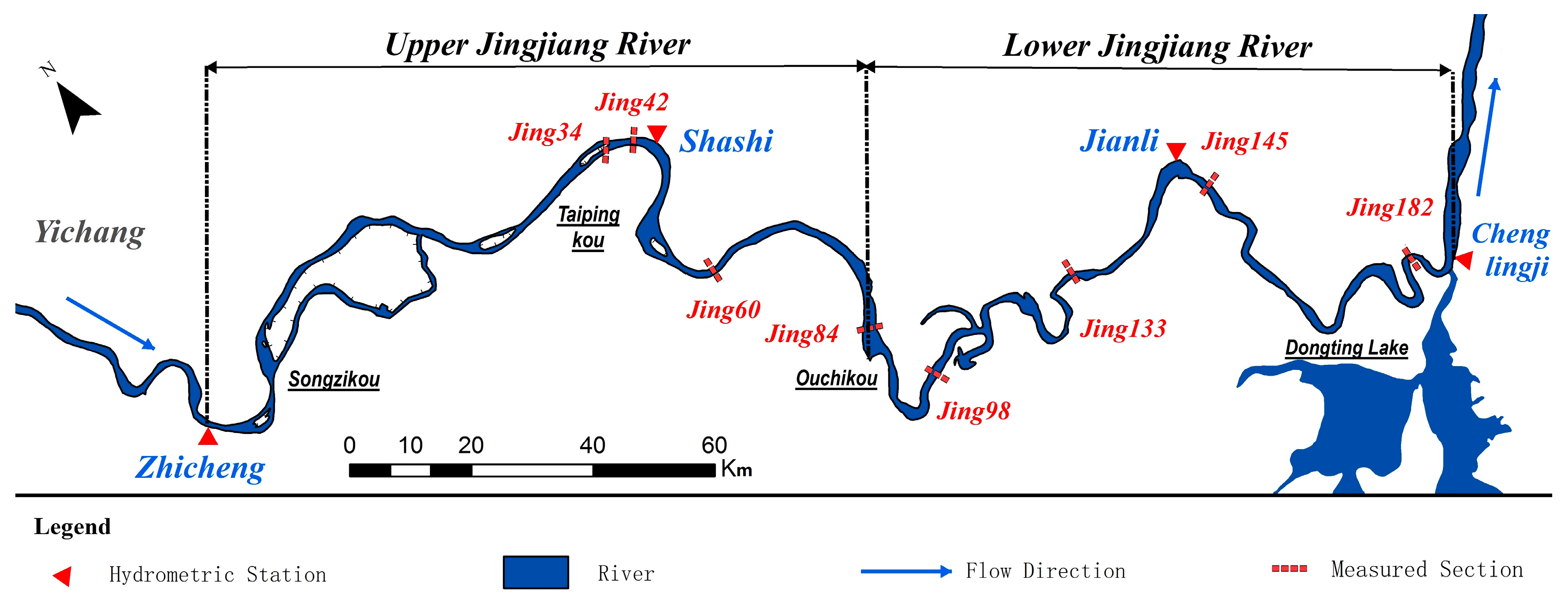
Figure 2.
Vertical distributions of sediment concentrations at Shashi and Jianli hydrological stations; data measured before (a) and after (b) the Three Gorges Dam (TGD) operation in 2003. Si is the measured concentration of the vertical profile (kg/m3), and Savg represents the vertical averaged concentration (kg/m3).
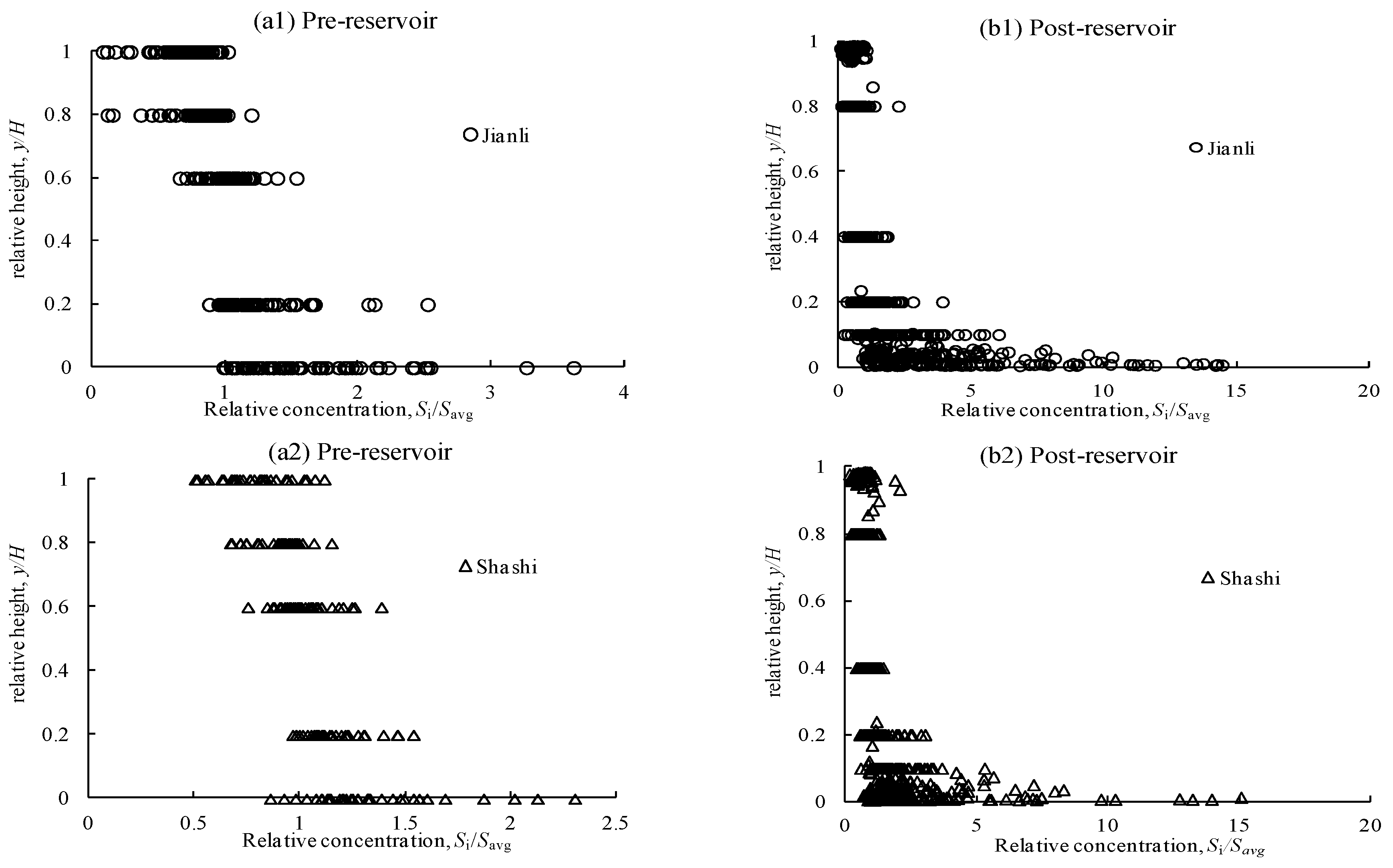
Figure 3.
Vertical distribution of sediment concentration measured at different regions. Data at Yangtze Estuary are drawn from Zhang [20], data at Wuhan and Jiujiang River Reach are drawn from Tang et al. [22], data at Oujiangkou and Taizhou sea area are drawn from Dong et al. [21], and data at silty coast are drawn from Xia et al. [24]. Si is the measured concentration of the vertical profile (kg/m3), and Savg represents the vertical averaged concentration (kg/m3).
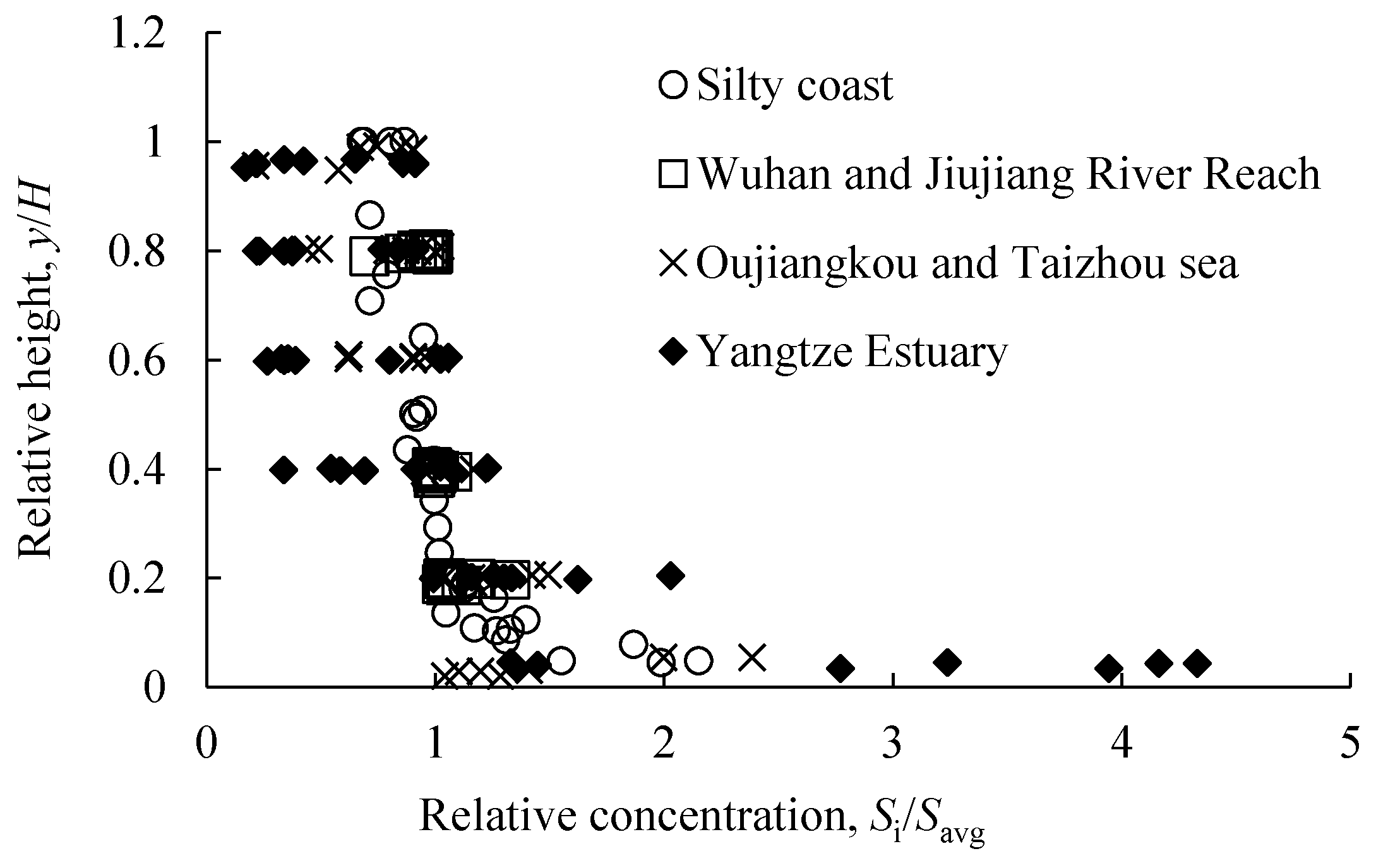
Figure 4.
Vertical concentrations comparing with near-bed point concentration at Shashi (a) and Jianli (b) hydrological stations (data measured after dam operation). Si = measured concentration of the vertical profile (kg/m3), and Sia = measured concentration of the near-bed point (kg/m3).
Figure 4.
Vertical concentrations comparing with near-bed point concentration at Shashi (a) and Jianli (b) hydrological stations (data measured after dam operation). Si = measured concentration of the vertical profile (kg/m3), and Sia = measured concentration of the near-bed point (kg/m3).

Figure 5.
Typical vertical profiles of type I (a) and type II (b) with tailing phenomena. The legends are composed of station name, date of measurement, and lateral distance of vertical line from left bank. Si = measured concentration of the vertical profile (kg/m3), and Sia = measured concentration of the near-bed point (kg/m3).

Figure 6.
Vertical distribution of Si/Sia with different ω/u*, (a) for (ω/u*) > 0.05 and (b) for (ω/u*) < 0.0001. ω = settling velocity, u* = over shear velocity, Si = measured concentration of the vertical profile (kg/m3), and Sia = measured concentration of the near-bed point (kg/m3).
Figure 6.
Vertical distribution of Si/Sia with different ω/u*, (a) for (ω/u*) > 0.05 and (b) for (ω/u*) < 0.0001. ω = settling velocity, u* = over shear velocity, Si = measured concentration of the vertical profile (kg/m3), and Sia = measured concentration of the near-bed point (kg/m3).

Figure 7.
Lateral distribution of contribution ratios of the two near-bed points, (a) for Shashi hydrological station, and (b) for Jianli hydrological station. R0 = contribution ratio of the two near-bed points, Bi = lateral distance of measured vertical lines from the left bank, and Bavg = maximum width of the cross section.
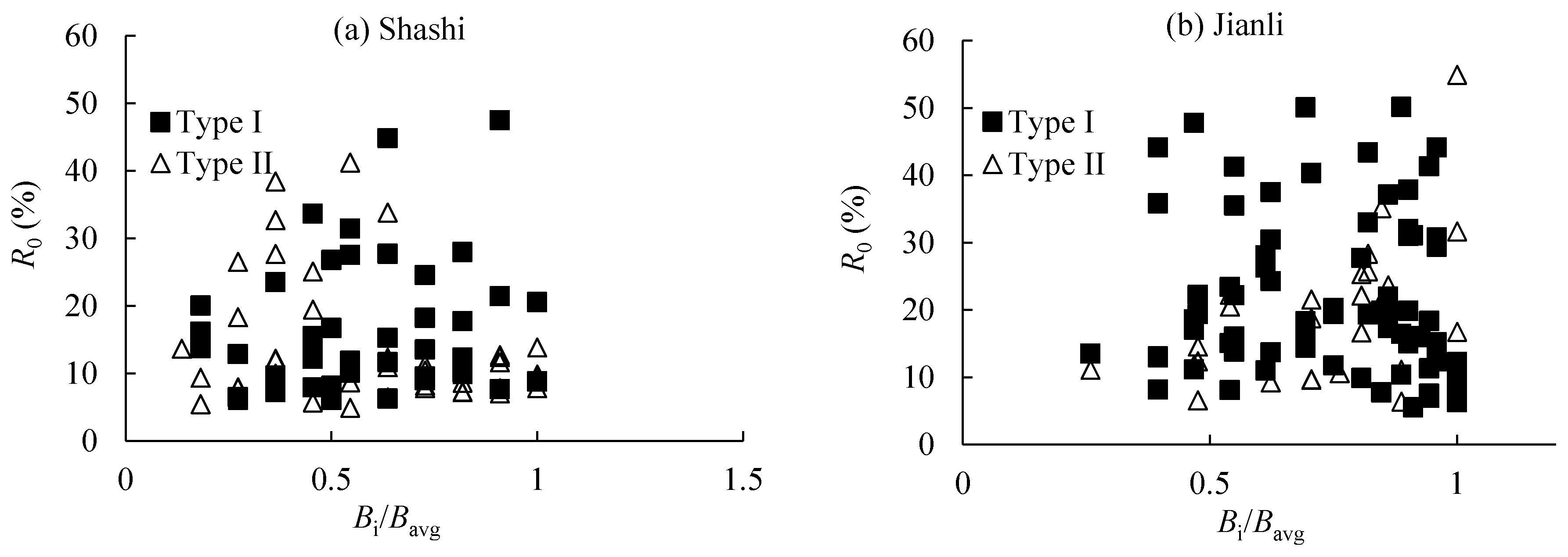
Figure 8.
Relationship between R0, ω/u* and particle diameters, (a) d < 0.02 mm, (b) 0.02 mm < d < 0.06 mm, and (c) d > 0.06 mm. The legends are the values of ω/u*. R0 = contribution ratio of the two near-bed points, ω = settling velocity, and u* = shear velocity.
Figure 8.
Relationship between R0, ω/u* and particle diameters, (a) d < 0.02 mm, (b) 0.02 mm < d < 0.06 mm, and (c) d > 0.06 mm. The legends are the values of ω/u*. R0 = contribution ratio of the two near-bed points, ω = settling velocity, and u* = shear velocity.
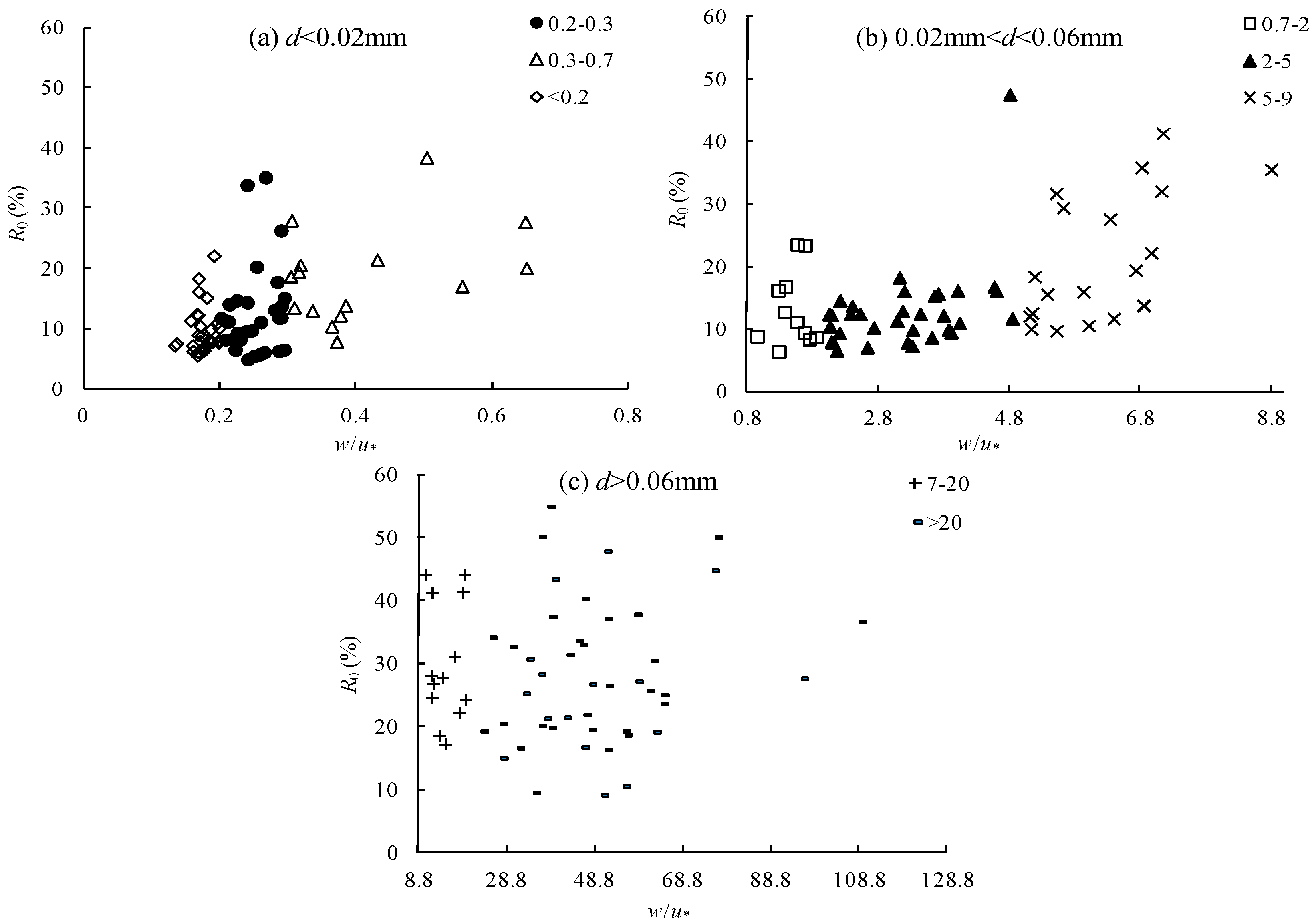
Figure 9.
Deviation ratio of sediment transport rate by data measured after TGD dam operation. The two ellipses indicate non-flood season and flood season, respectively. R = contribution ratio of the two near-bed points on vertical sediment flux.
Figure 9.
Deviation ratio of sediment transport rate by data measured after TGD dam operation. The two ellipses indicate non-flood season and flood season, respectively. R = contribution ratio of the two near-bed points on vertical sediment flux.
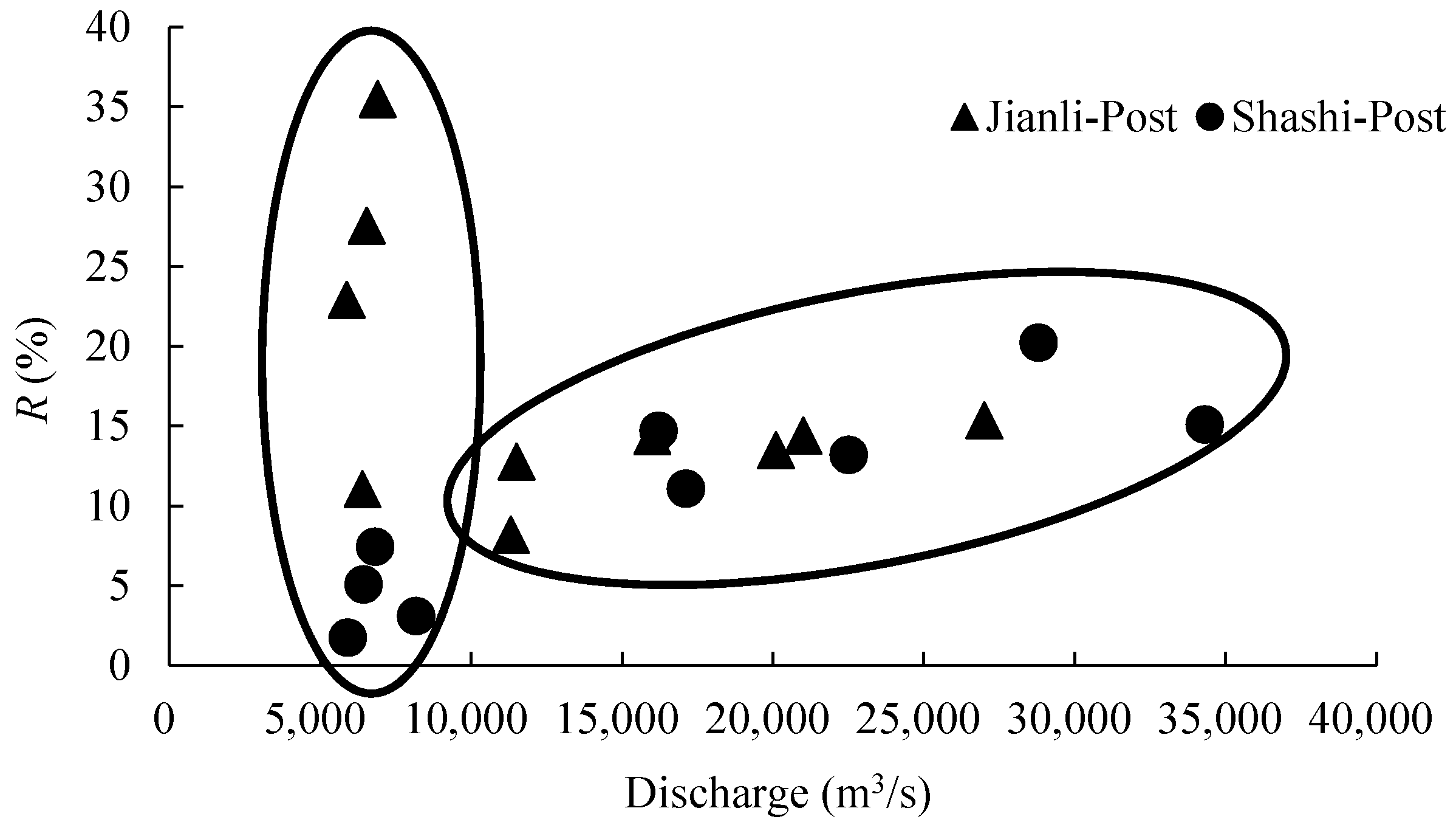
Figure 10.
Contributing ratios of near-bed sediment concentration on total deposition estimation, at three sites, (a) the Yichang–Zhicheng, (b) the Zhicheng–Shashi, and (c) the Sahshi–Jianli reaches, based on data measured during 2002–2008 (from Yuan et al. [26]).
Figure 10.
Contributing ratios of near-bed sediment concentration on total deposition estimation, at three sites, (a) the Yichang–Zhicheng, (b) the Zhicheng–Shashi, and (c) the Sahshi–Jianli reaches, based on data measured during 2002–2008 (from Yuan et al. [26]).
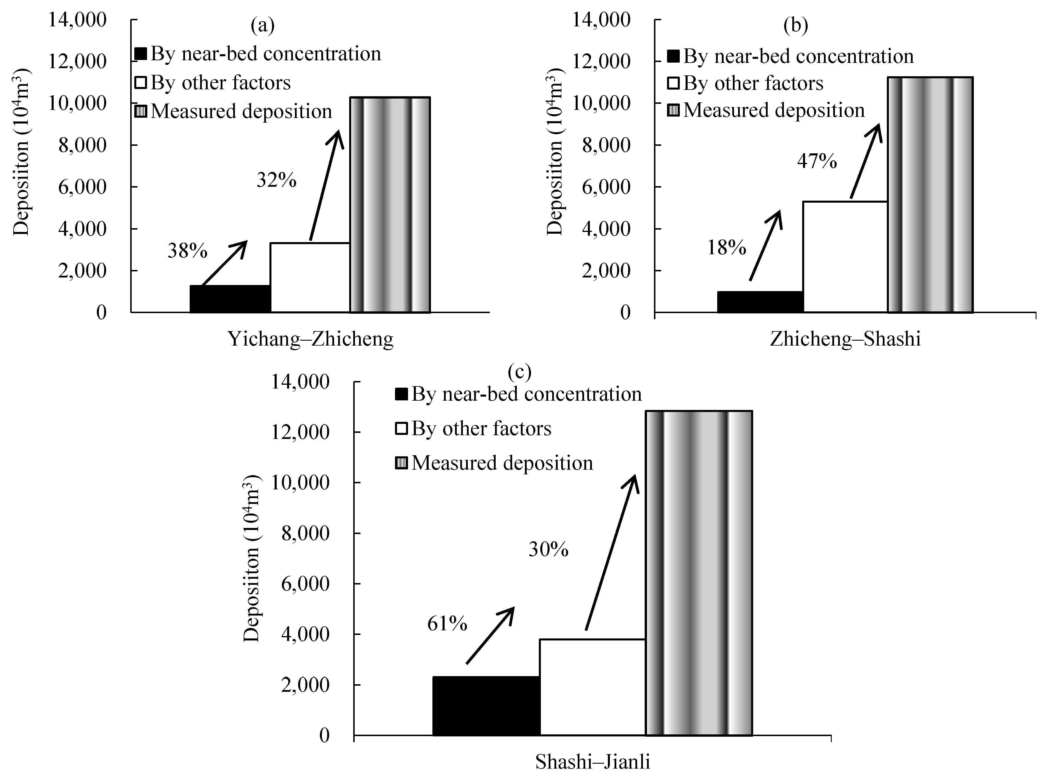
Figure 11.
Calculated vertical sediment concentrations comparing with near-bed point concentration (After Zhang and Tan [30]). Si = measured concentration of the vertical profile (kg/m3), and Sia = measured concentration of the near-bed point (kg/m3).
Figure 11.
Calculated vertical sediment concentrations comparing with near-bed point concentration (After Zhang and Tan [30]). Si = measured concentration of the vertical profile (kg/m3), and Sia = measured concentration of the near-bed point (kg/m3).
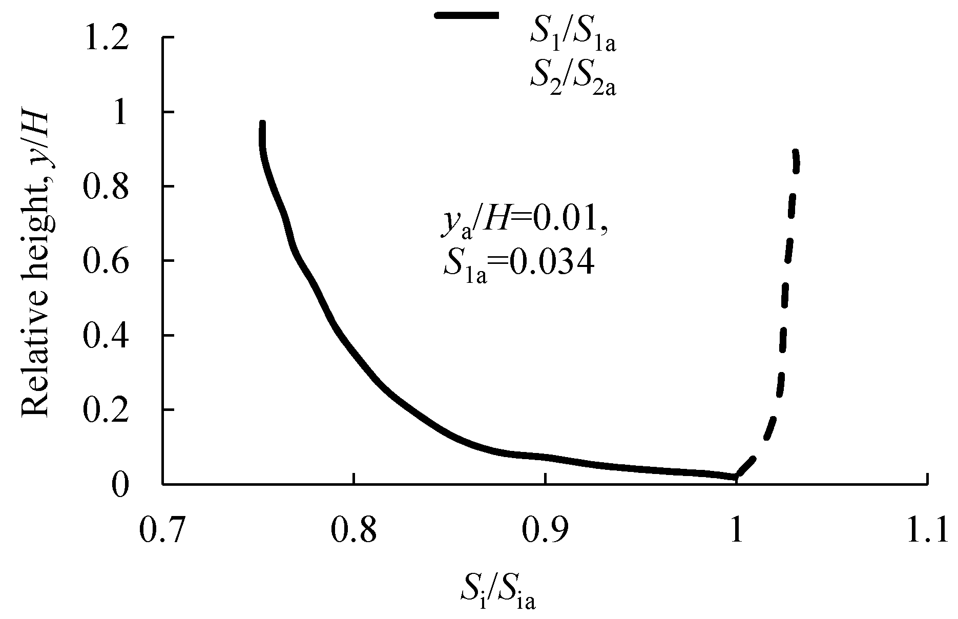
Figure 12.
Percentages of particle groups before and after TGD dam operation at Shashi (a) and Jianli (b) hydrological stations. Data for pre-reservoir are average values between 1991 and 2002, and data for post-reservoir are average values between 2003 and 2016.
Figure 12.
Percentages of particle groups before and after TGD dam operation at Shashi (a) and Jianli (b) hydrological stations. Data for pre-reservoir are average values between 1991 and 2002, and data for post-reservoir are average values between 2003 and 2016.
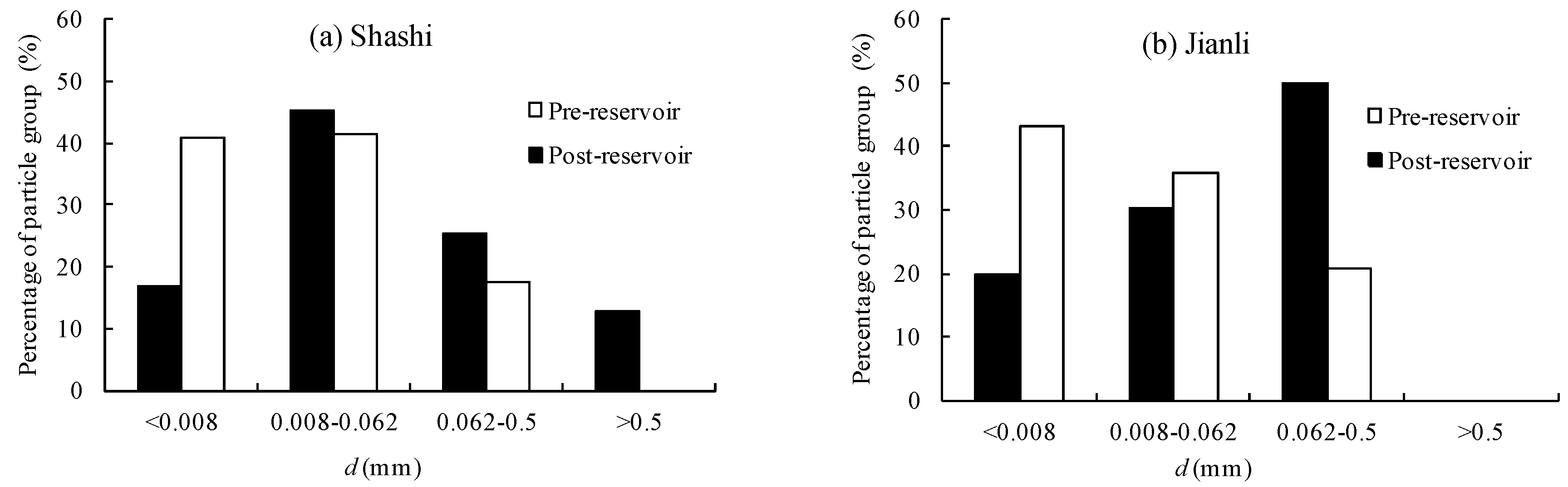
Figure 13.
Bed load of Shashi (a) and Jianli (b) hydrological stations. Data in (a) were measured 9 July 1986 at Xinchang hydrological station, and 6 June 2013 at Shashi hydrological station; data in (b) were measured 26 May 1986 and 13 March 2013 at Jianli hydrological station.
Figure 13.
Bed load of Shashi (a) and Jianli (b) hydrological stations. Data in (a) were measured 9 July 1986 at Xinchang hydrological station, and 6 June 2013 at Shashi hydrological station; data in (b) were measured 26 May 1986 and 13 March 2013 at Jianli hydrological station.
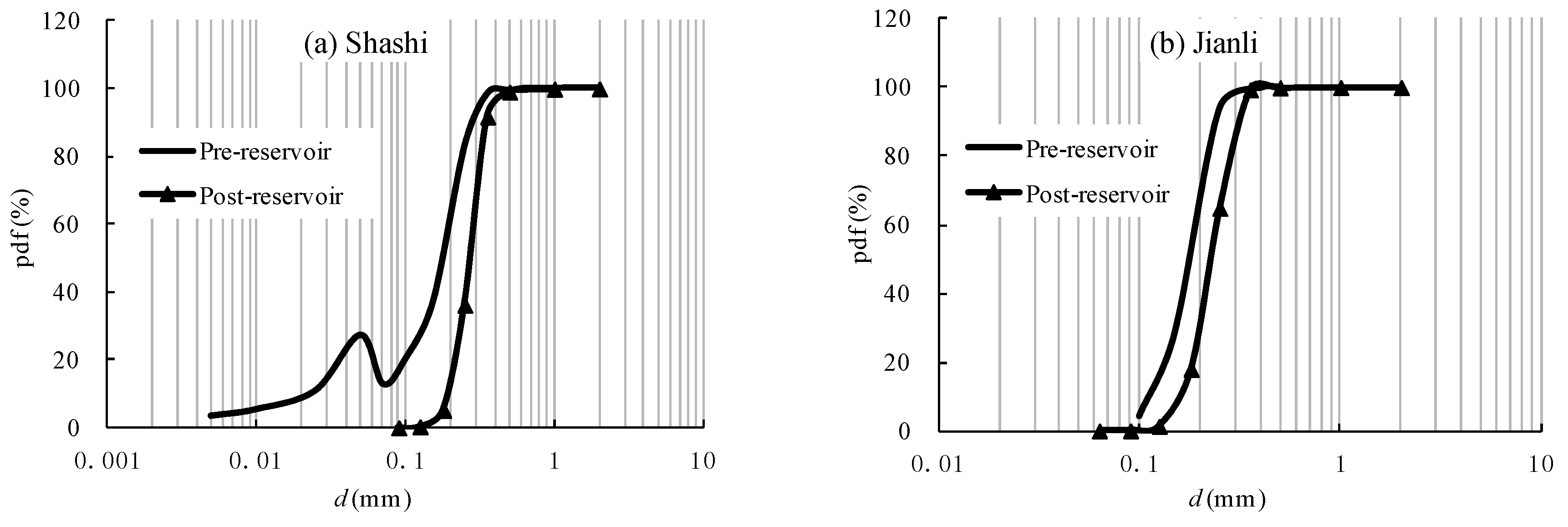
Figure 14.
Deviation ratio of sediment transport rate by data measured before TGD dam operation. The two ellipses indicate non-flood season and flood season, respectively. R = contribution ratio of the two near-bed points on vertical sediment flux.
Figure 14.
Deviation ratio of sediment transport rate by data measured before TGD dam operation. The two ellipses indicate non-flood season and flood season, respectively. R = contribution ratio of the two near-bed points on vertical sediment flux.
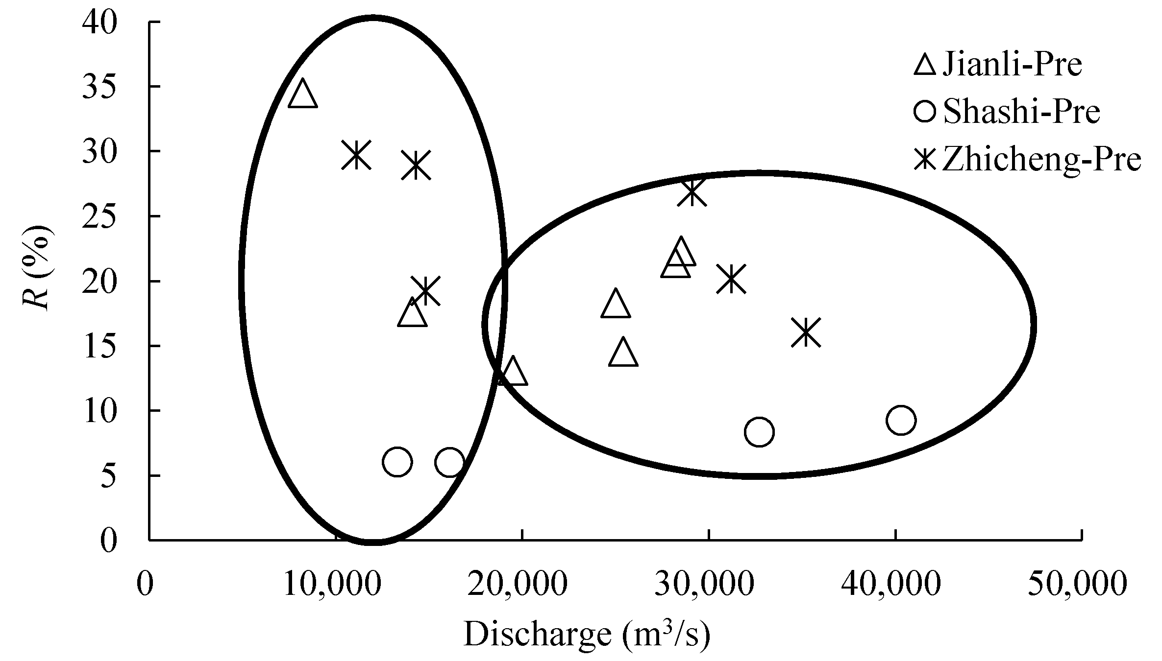
Figure 15.
Comparison between measured and calculated sectional discharge (a) and concentration (b).
Figure 15.
Comparison between measured and calculated sectional discharge (a) and concentration (b).
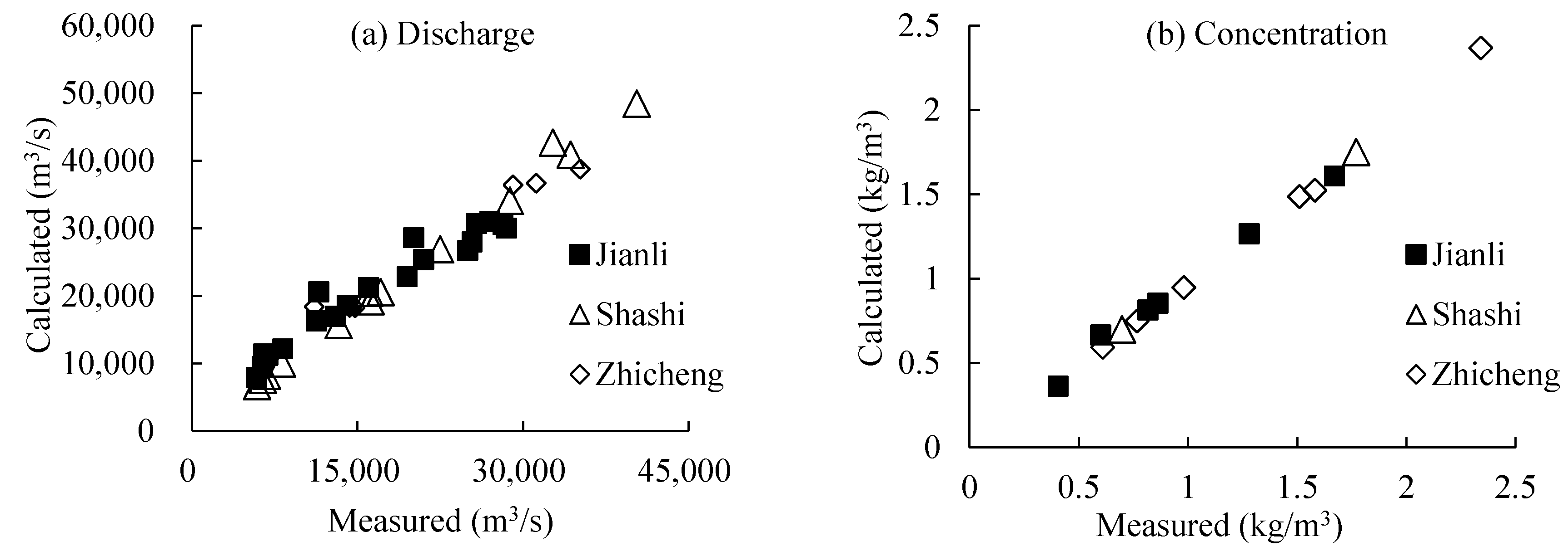
Figure 16.
Sediment regimes of floods occurring before and after the operation of the TGD, the Jingjiang River Reach. (a) for Shashi Hydrological Station, and (b) for Jianli Hydrological Station, S = average concentration, and S* = average carrying capacity.
Figure 16.
Sediment regimes of floods occurring before and after the operation of the TGD, the Jingjiang River Reach. (a) for Shashi Hydrological Station, and (b) for Jianli Hydrological Station, S = average concentration, and S* = average carrying capacity.

Table 1.
Statics of data measured at the Jingjiang River Reach.
| Stations | Measured Year | Groups |
|---|---|---|
| Zhicheng | 1996, 1998, 2002 | 55 |
| Shashi | 1996, 1998, 2010, 2011, 2012, 2013 | 130 |
| Jianli | 1986, 1998, 2002, 2010, 2011, 2012, 2013 | 180 |
Table 2.
Characteristics of vertical profiles of Type I and Type II measured at Shashi and Jianli hydrological stations (after dam operation).
Table 2.
Characteristics of vertical profiles of Type I and Type II measured at Shashi and Jianli hydrological stations (after dam operation).
| Stations | Type I | Type II | ||||||||||
|---|---|---|---|---|---|---|---|---|---|---|---|---|
| Flood Season | Non-Flood Season | Flood Season | Non-Flood Season | |||||||||
| Amount of Group | Range of (ω/u*) | D50 (mm) | Amount of Group | Range of (ω/u*) | D50 (mm) | Amount of Group | Range of (ω/u*) | D50 (mm) | Amount of Group | Range of (ω/u*) | D50 (mm) | |
| Shashi | 33 | 0.16–95.38 | 0.01 | 17 | 2.09–108.89 | 0.06 | 20 | 0.16–1.37 | 0.03 | 25 | 1.84–95.67 | 0.07 |
| Jianli | 47 | 0.14–76.15 | 0.06 | 29 | 2.38–61.64 | 0.10 | 10 | 0.13–32.58 | 0.06 | 19 | 1.38–63.92 | 0.10 |
Table 3.
Vertical averaged R0-values of data measured after TGD dam operation.
| Stations | Type I | Type II | ||
|---|---|---|---|---|
| Flood Season | Non-Flood Season | Flood Season | Non-Flood Season | |
| Shashi | 15.67 | 21.28 | 12.51 | 14.10 |
| Jianli | 19.57 | 27.70 | 16.94 | 19.61 |
Table 4.
Sectional averaged R-values of data measured after TGD dam operation.
| Stations | Total | Flood Season | Non-Flood Season |
|---|---|---|---|
| Shashi | 10.21 | 14.88 | 4.36 |
| Jianli | 17.56 | 13.10 | 24.24 |
Table 5.
Characteristics of vertical profiles measured at Shashi and Jianli hydrological stations before TGD dam operation.
Table 5.
Characteristics of vertical profiles measured at Shashi and Jianli hydrological stations before TGD dam operation.
| Stations | Flood Season | Non-Flood Season | ||
|---|---|---|---|---|
| Amount of Group | Range of (ω/u*) | Amount of Group | Range of (ω/u*) | |
| Shashi | 27 | 0.08–0.46 | 9 | 0.23–1.34 |
| Jianli | 53 | 0.02–0.78 | 22 | 0.05–12.12 |
Table 6.
Sectional averaged R-values of data measured before TGD dam operation.
| Stations | Total | Flood Season | Non-Flood Season |
|---|---|---|---|
| Zhicheng | 23.50 | 21.04 | 25.86 |
| Shashi | 7.43 | 8.81 | 6.04 |
| Jianli | 32.95 | 17.96 | 45.93 |
Table 7.
Characteristics of major floods in China in 1998 (Data adapted from Zhou and Chen [41]).
Table 7.
Characteristics of major floods in China in 1998 (Data adapted from Zhou and Chen [41]).
| Stations | Flood Volumes 109 m3 | Maximum Peak Flow Discharge | Maximum Flood Stage | |||
|---|---|---|---|---|---|---|
| In 30 Days | In 60 Days | Discharge (m3/s) | Date | Stage (m) | Date | |
| Yichang | 137.9 | 254.5 | 63,600 | 16/8 | 54.49 | 16/8 |
| Shashi | – | – | 53,700 | 17/8 | 45.22 | 17/8 |
| Jianli | – | – | 45,200 | 17/8 | 38.31 | 17/8 |
| Luoshan | – | – | 68,600 | 27/7 | 34.95 | 20/8 |
| Hankou | 175.4 | 336.5 | 72,300 | 19/8–20/8 | 29.43 | 20/8 |
| Jiujiang | – | – | – | – | 23.03 | 2/8 |
| Datong | 202.7 | 395.1 | 82,300 | – | 16.32 | 2/8 |
| Nanjing | – | – | – | – | 10.14 | 29/7 |
Table 8.
Instruments, methods and criteria adopted in the field survey.
| Measuring | Instruments or Methods | Criteria or Error |
|---|---|---|
| Positioning of instrument | Total station Digital Level | Positioning error: ±0.3 m (vertical), ±1.5 m (vertical lines) |
| Vertical lines for measuring velocity | RTK–GNSS (antenna and receiver) | Position errors of antenna: 0.5° RMS (orientation) and 0.5–3 m RMS (position). Position errors of receiver: ±10 mm + 1 ppm (horizontal), ±20 mm + 1 ppm (vertical), where ppm means additional error per km of baseline. |
| Velocity | Acoustic Doppler Current Profilers (ADCP) | The deviation between each measured discharge and the averaged discharge should be less than ±5%, otherwise, data should be re-measured. |
| Water depth | ADCP | Verified with fish lead. Frequency: 600 KHz Sounding range: 0.7–75 m Velocity measurement: ±20 m/s Resolution: 0.1 cm/s |
| Sampling Suspended sediment | Bottom-touched automatic-closing sampler | The dropping speed of the sampler is reduced when approaching the riverbed. The sampler may close automatically when it is brought into contact with the riverbed. |
| Suspended sediment gradation | Sieving method | Field (2 mm, 5 mm, 10 mm, 25 mm, 50 mm, 75 mm, 100 mm, 150 mm, 200 mm, 250 mm, and 300 mm) Lab (0.002 mm, 0.004 mm, 0.008 mm, 0.016 mm, 0.032 mm, 0.062 mm, 0.125 mm, 0.25 mm, 0.5 mm, 1.0 mm, and 2.0 mm) |
| Near-bed concentration | Double-checked after sampling and grain-size analysis | The measured concentration is reliable when the vertical profiles of concentration of particles with d50 < 0.062 mm has no changing point in near-bed region. Otherwise, related measurements should be omitted. |
© 2017 by the author. Licensee MDPI, Basel, Switzerland. This article is an open access article distributed under the terms and conditions of the Creative Commons Attribution (CC BY) license (http://creativecommons.org/licenses/by/4.0/).
Share and Cite
MDPI and ACS Style
He, L. Quantifying the Effects of Near-Bed Concentration on the Sediment Flux after the Operation of the Three Gorges Dam, Yangtze River. Water 2017, 9, 986. https://doi.org/10.3390/w9120986
AMA Style
He L. Quantifying the Effects of Near-Bed Concentration on the Sediment Flux after the Operation of the Three Gorges Dam, Yangtze River. Water. 2017; 9(12):986. https://doi.org/10.3390/w9120986
Chicago/Turabian StyleHe, Li. 2017. "Quantifying the Effects of Near-Bed Concentration on the Sediment Flux after the Operation of the Three Gorges Dam, Yangtze River" Water 9, no. 12: 986. https://doi.org/10.3390/w9120986
Note that from the first issue of 2016, this journal uses article numbers instead of page numbers. See further details here.