A Comparison of Preference Handling Techniques in Multi-Objective Optimisation for Water Distribution Systems
by
Gilberto Reynoso-Meza
1,*,†, 
Victor Henrique Alves Ribeiro
1,† and
Elizabeth Pauline Carreño-Alvarado
2,† 1
Industrial and Systems Engineering Graduate Program (PPGEPS), Pontifical Catholic University of Parana (PUCPR), Curitiba 80215-901, Brazil
2
Department of Hydraulic and Environmental Engineering, Universitat Politènica de Valècia, 46022 Valencia, Spain
*
Author to whom correspondence should be addressed.
†
These authors contributed equally to this work.
Water 2017, 9(12), 996; https://doi.org/10.3390/w9120996
Submission received: 31 October 2017
/
Revised: 22 November 2017
/
Accepted: 24 November 2017
/
Published: 19 December 2017
(This article belongs to the Special Issue Advanced Hydroinformatic Techniques for the Simulation and Analysis of Water Supply and Distribution Systems)
Abstract
:Dealing with real world engineering problems, often comes with facing multiple and conflicting objectives and requirements. Water distributions systems (WDS) are not exempt from this: while cost and hydraulic performance are usually conflicting objectives, several requirements related with environmental issues in water sources might be in conflict as well. Commonly, optimisation statements are defined in order to address the WDS design, management and/or control. Multi-objective optimisation can handle such conflicting objectives, by means of a simultaneous optimisation of the design objectives, in order to approximate the so-called Pareto front. In such algorithms it is possible to embed preference handling mechanisms, with the aim of improving the pertinency of the approximation. In this paper we propose two mechanisms to handle such preferences based on the TOPSIS (Technique for Order of Preference by Similarity to Ideal Solution) and PROMETHEE (Preference Ranking Organisation METHod for Enrichment of Evaluations) methods. Performance evaluation on two benchmarks validates the usefulness of such approaches according to the degree of flexibility to capture designers’ preferences.
1. Introduction
Dealing with real world engineering problems often comes with facing multiple and conflicting objectives and requirements. Water distributions systems (WDS) are not exempt from this: while cost and hydraulic performance are usually conflicting objectives, several requirements related with environmental issues in water sources might be in conflict as well. Commonly, optimisation statements are defined in order to address the WDS design, management and/or control. Nevertheless, such problems become difficult since, besides their multi-objective conflicting nature, the optimisation problem might be non-linear (due to head-loss relationships for example) and/or discrete combinatorial (due to standardisation of pipe parameters) [1,2].
Multi-objective optimisation [3] can handle such an issue, by means of a simultaneous optimisation of the design objectives. At the end of this process, a potential set of solutions, the Pareto front, is approximated. In this set of solutions, there is not a best solution, but a preferable solution. This means that several solutions are calculated, with different trade-offs between conflicting objectives and the engineer will select among them the most preferable for the problem at hand.
Given that several solutions are calculated, the designer must perform a decision making stage. In this stage, it is required to express somehow the preferences according to the trade-offs, in order to select the most suitable (preferable) solution for the problem at hand. This might not be a trivial task, since most of the times to interpret such trade-offs is not easy, given the multidimensional structure of the problem. Therefore, visualisation techniques [4] and multi-criteria decision making methodologies are valuable and helpful for designers.
It is possible to use different decision making methodologies, such as TOPSIS [5] (Technique for Order of Preference by Similarity to Ideal Solution), Physical Programming [6], PROMETHEE [7] (Preference Ranking Organisation METHod for Enrichment of Evaluations), among others. While it is usual to apply such methodologies in the decision making step, it is also possible to embed them into the optimisation process. For example, the Physical Programming method has been used before in order to evolve the population of a multi-objective evolutionary algorithm (MOEA) towards the pertinent region of the objective space [8,9]. With such approach, it is possible to use preference-information actively in the optimisation, improving the usability of the approximated Pareto front, as well as dealing with more than 3 design objectives effectively. In this paper some modifications are proposed, incorporating the TOPSIS and the PROMETHEE mechanism for the same purpose in a MOEA.
The remainder of this paper is as follows: in Section 2 a review on multi-objective optimisation techniques for WDS is presented, identifying the necessity of preference handling techniques. In Section 3 the TOPSIS and PROMETHEE methods are incorporated into a MOEA for preference handling and they are evaluated in Section 4 with two MOPs. Finally, conclusions of this work are commented.
2. Review
A literature review on the optimisation of WDS is presented in [2], where the authors bring together over two hundred journal publications from the past three decades. From those publications, the authors create a table with substantial information from over one hundred of them, from which seventeen papers focus on the use of a MOO approach. The first papers on MOO for WDS focused solely on the optimisation of operation and maintenance costs. Next, the optimisation of water quality became the main interest by some researchers. Nowadays, research on the subject focuses on finding the trade-off between cost and water quality. A review of each paper is presented below, followed by Table 1, which resumes the MOO design characteristics of each publication. Background and definitions of the MOO process are presented in the Appendix for interested readers.
A multi-objective hybrid approach of the Genetic Algorithm (GA) is introduced by [10] to find the trade-off between the minimisation of: (a) energy; and (b) maintenance costs on a net with four pumps and one reservoir. One set of binary decision variables is used for this problem, which indicates the pump statuses for each hour on a twenty-four hours period. The recovery of the initial reservoir water level at the end of the simulation period is used as the equality constraint, while the minimum and maximum reservoir levels are set as inequality constraints.
A simplified system, composed of one source, five pumps and one elevated reservoir is the object of study by [11], where strength Pareto evolutionary algorithm (SPEA), using one set of binary decision variables for the pump statuses, finds the trade-off between the minimisation of the: (a) pump operating costs; (b) number of pump switches; (c) difference between initial and final levels in the reservoir; and (d) maximum daily power peak. The problem contains four inequality constraints: (a) minimum reservoir water levels; (b) maximum reservoir water levels; (c) minimum pipeline pressure; and (d) maximum pipeline pressure. At the end of the paper, a two-dimensional Pareto front is presented.
A WDS from Belgium is optimised by [12] using a multi-objective genetic algorithm (MOGA) with penalised tournament selection scheme, where two objectives are minimised: (a) the pump operating costs; and (b) the number of pump switches. Three sets of decision variables are defined: (a) the binary pump statuses; (b) the rotating speed of the pumps; and (c) the pressure loss coefficient for the control valve. The problem is composed of two sets of equality constraints: (a) the initial reservoir water level must be reached by the end of the optimisation; and (b) the consumer demands must be satisfied at any period of time. In addition, two sets of inequality constraints must be met: (a) the maximum; and (b) the minimum water levels for each reservoir. The authors plot a two-dimensional Pareto front, but do not choose a preferred solution.
A comparison of six MOO algorithms is performed by [13] using the same WDS from [11]. The compared algorithms are: SPEA, non-dominated sorting algorithm (NSGA), NSGA-II, controlled elitist non-dominated sorting genetic algorithm (CNSGA), niched Pareto genetic algorithm (NPGA), and MOGA. The MOP is designed with four objectives, the minimisation of: (a) pump operating costs; (b) number of pump switches; (c) difference between initial and final water levels in the reservoir; and (d) maximum daily power peak. Only one set of decision variables is used, the binary pump statuses, while four inequality constraints are used: (a) the minimum reservoir water levels; (b) the maximum reservoir water levels; (c) the minimum pipeline pressure; and (d) the maximum pipeline pressure. The algorithms are compared by six different metrics: (a) overall non-dominated vector generation; (b) overall non-dominated vector generation ratio; (c) error ratio; (d) generational distance; (e) maximum Pareto front error; and (f) spacing.
The simulation of a small WDS is optimised by [14] using the second version of SPEA, the SPEA2. One set of decision variables, the binary pump status, is used to find the trade-off between two objectives, the minimisation of: (a) pump operating costs; and (b) number of pump switches. One equality constraint is used, the pressure at demand nodes, while three inequality constraints are used: (a) maximum tank water levels; (b) minimum tank water levels; and (c) tank volume deficit at the end of the simulation. The authors compare the Pareto fronts of four different methods for the initial population generation, using scatter plots and the attainment surfaces as the metric.
A real-time pump scheduling framework is proposed by [15], where optimisation is performed using a multialgorithm genetically adaptive method (AMALGAM). The framework is applied to a WDS from Brazil, and the MOP is composed of two objectives: (a) the minimisation of pump operating costs; and (b) maximisation of operational reliability. One set of decision variables, the binary pump status, is considered. Three sets of inequality constraints are used: (a) the minimum pressure at any network node; (b) the tank water levels at the end of the scheduling period; and (c) the maximum number of pump switches. In addition, one equality constraint, where the occurrence of simulation errors must be equal to zero, is considered. The authors present the resulting Pareto front on a two-dimensional scatter plot.
Seven different scenarios are optimised by [16] using NSGA-II. Each scenario is composed of different emission factors and time horizons. The MOP is composed of one set of decision variables, the pump schedules, and two objectives, the minimisation of: (a) pump operating costs; and (b) greenhouse gas emissions associated with the use of electricity from fossil fuel sources. Two sets of inequality constraints are considered: (a) the minimum pressure at network nodes; and (b) minimum total volume of water pumped into each district metered area. The authors present the Pareto fronts on two-dimensional scatter plots, and the solutions selected for analysis are based on minimum values for both objectives.
The simulation of a real water utility network is subject to MOO by [17] using NSGA-II, where the trade-off between two objectives: (a) the minimisation of the total disinfectant dose; and (b) the maximisation of the volumetric percentage of water supplied with disinfectant residuals, is found. Two decision variables are used in this optimisation: (a) the locations of booster disinfection stations; and (b) the disinfection injections schedules. In addition, three inequality constraints are used: (a) non-negative disinfectant doses; (b) lower bound on the value of the Objective (b); and (c) upper bound on disinfectant concentrations at monitoring nodes. An analysis of the Pareto front is made by the authors using scatter plots.
The Pareto front of a WDS is found by [18] using NSGA-II. The MOP is elaborated with three objectives, the minimisation of: (a) the number of chlorine booster stations; (b) mean value of chlorine concentrations; and (c) mean value of instances not meeting quality requirements. In addition, two decision variables are used: (a) the presence of a booster stations at a network node; and (b) the chlorine concentrations at booster stations and treatment plants. In total, five inequality constraints are used in this problem: (a) the maximum number of booster stations; and (b) the minimum number of booster stations; (c) the maximum shlorine concentration and (d) the minimum chlorine concentrations; and (e) the minimum chlorine concentration at treatment plants. By the end of the paper, the authors present a scatter plot of the Objectives (b) and (c), which are grouped by the values of Objective (a).
A WDS from Poland is optimised by [19] using a distributed MOGA, based on the island GA. The problem is composed of the same objectives and decision variables presented by [18], but only uses the first four inequality constraints. The resulting Pareto front is presented by a two-dimension scatter plot of objectives (b) and (c) grouped by values of objective (a).
Two case studies are optimised by [20] using NSGA-II, one hypothetical and one simulation of a WDS from Colombia. For both cases, the objectives are defined as the minimisation of: (a) the number of polluted nodes; and (b) the number of the operational interventions needed. Only one set of decision variables is used for this problem, the operational interventions on pumps, valves and switches. In total, three sets of constraints are used on this publication, two inequality constraints, where: (a) nodes pressures must be positive; and (b) technical operational capacity for interventions must be met, and one equality constraint, where network connectivity must be ensured. The resulting Pareto front is presented as a two-dimensional scatter plot.
The optimisation of a WDS is performed by [21] using the optimised MOGA (OPTIMOGA). The MOP is composed of four inequality constraints: (a) the minimum pressure for sufficient pressure, expressed by the number of times which it is not satisfied; (b) the tank volume deficit at the end of the simulation; (c) the minimum tank levels, expressed as the times which it is not satisfied; and (d) the maximum tank levels. It is also composed of one equality constraint, the global mass balance in each tank (there is only one tank in the case study). One set of decision variables, the binary status of the pumps and gates, is used to minimise two objective functions. The first objective is an aggregate function of: (a) pump operating costs; and (b) water losses cost; and the second is the function of Inequality Constraints (a), (b) and (c). The authors present a table with the resulting Pareto front of the problem, and one solution is selected for being the only feasible solution.
Two multi-objective optimisation algorithms, based on the harmonic search algorithm (HSA), are developed by [22] in order to solve a pump scheduling problem, the multi-objective HSA (MO-HSA) and the polyphonic HSA (Poly-HSA). The MO-HSA is used to optimise an operational pumping field from Paraguay, and the problem is composed by the minimisation of four objectives: (a) pump operating costs; (b) quantity of pumped water; (c) electric energy peak consumption; and (d) number of pump switches. The optimisation is executed two times, Once with Objectives (a), (b) and (c), and again with Objectives (a), (b), and (d). The problem is also composed of one set of decision variables, the binary pump status, and four sets of inequality constraints, used within a penalty mechanism. Such constraints are: (a) the minimum water levels in storage tanks; and (b) the maximum water level in storage tanks; and the (c) the minimum volume deficit in the storage tanks at the end of the scheduling period; and (d) the maximum volume deficit in the storage tanks at the end of the scheduling period. The authors present, for both runs, a three-dimensional scatter plot with the Pareto front.
Two optimisation problems, one related to chlorine concentrations, and another related to water age, are solved by [23] using SPEA2. In total, four objectives are defined for the MOP, the minimisation of: (a) pump operating costs; (b) disinfectant concentrations at monitoring nodes; (c) water age for demand nodes; and (d) cost of tanks. The first optimisation model includes Objectives (a), (b) and (c), while the second model includes Objectives (a), (c) and (d). Three sets of decision variables are used for this problem: (a) the pump speeds; (b) the disinfectant concentrations at treatment plants; and (c) tank diameters. One equality constraint, the pressure at nodes, and three inequality constraints: (a) the minimum volume deficit at the end of the simulation; (b) the maximum volume surplus at the end of the simulation; and (c) the minimum amount of stored water at any time, are used in both optimisation models. The resulting Pareto fronts are presented on three-dimensional scatter plots, and three solutions are selected for each Pareto, one “balanced” solution, which is the closest an Utopian solution, and the other two are related to minimal values for Objectives (a) and (b).
The optimisation of two systems is performed in [24] using SPEA2 and the MOP defined in [23], but only the first two objectives and decision variables are used. The authors present a two-dimensional scatter plot for both examples, and a single “balanced” solution is selected on the MCDM stage, but no metrics were specified.
A total of fourteen different scenarios are optimised by [25] using NSGA-II. All scenarios are defined as a MOP with two objectives, the minimisation of: (a) pump operating costs; and (b) deviations of the actual constituent concentrations from the required values. For such problems, one set of decision variables, the binary pump status, are defined. Furthermore four sets of inequality constraints are considered: (a) the minimum pressure at customer nodes; (b) the minimum water level in the storage tanks; (c) the maximum water level in the storage tanks; and (d) the volume deficit in the storage tanks at the end of the scheduling period. The resulting Pareto front for all scenarios are presented on a two dimensional scatter plot and, for comparison with results from the literature, one “balanced” solution is selected for analysis, but no metrics were specified.
Six different scenarios based on a network with ninety-four nodes are optimised by [26] using NSGA-II. All scenarios are defined as a MOP with three objectives, the minimisation of: (a) pump operating costs; (b) the turbidity deviations from the allowed values; and (c) deviations of the actual constituent concentrations from the required values. Decision variables and constraints are defined as in [25]. The resulting Pareto fronts for all scenarios are presented on a three-dimensional scatter plot and three different two-dimensional scatter plots, for each two objectives combination, and two solutions were selected from two different scenarios for comparison purposes. No specific metrics were indicated for such selections.
In Table 1 a summary of such papers is shown. It is interesting to note that the vast majority of papers are focusing on MOPs with two or three design objectives. A possible reason for this might be the difficulties to perform a MCDM and to visualise the Pareto front approximation. For this reason, the idea of stating more than three design objectives for WDS is exploited in this paper, using different preference mechanisms to evolve towards the pertinent region of the Pareto front.
3. Proposal and Experiment Description
As it has been noticed before, tendencies regarding the number of design objectives for MOPs is to state two or three. One of the circumstances leading to this might be that any MOP with more than three design objectives is said to be a many-objectives MOP problem. In such an instance, mechanisms for diversity and convergence are in conflict. Therefore, additional mechanisms are often required in order to guarantee a suitable performance of the Pareto front approximation process. One of such mechanisms is the inclusion of preferences [27].
As it has been commented in the introduction, a MOEA using Physical Programming as preference handling mechanism, the sp-MODEII (Multi-Objective Differential Evolution with Spherical Pruning, version II) (Toolbox available at https://www.mathworks.com/matlabcentral/fileexchange/47035) has been proposed before [8,9]. The sp-MODEII is an evolutionary algorithm for multi-objective optimisation. Its main characteristics are:
- It uses spherical pruning [32] in order to promote diversity in the approximated Pareto front. Basically, the objective space is partitioned using spherical coordinates, and one solution is selected in each spherical sector, avoiding overcrowding areas.
- It uses physical programming (PP) [6] for pertinency improvement and as a mechanism for many-objectives optimisation. It states such preferences in aspiration levels in a matrix M as depicted in Table 2. This PP index is used as an additional mechanism to prune solutions, according to the preference index, in order to get a manageable size of the Pareto front approximation.
Nevertheless, in spite of its usefulness, different mechanisms might substitute the Physical Programming approach requiring less information from the designer. For this reason, we modify such an algorithm with two additional mechanisms for pertinency improvement (Available at: https://www.mathworks.com/matlabcentral/fileexchange/65145). The first of them the TOPSIS mechanism [5], and the second the PROMETHEE II [7] method. That is, the original pruning mechanism using Physical Programming is modified. While the TOPSIS mechanism just require as input the Pareto front approximation, the PROMETHEE II method require information about (in) significant differences for each design objective (See Table 3). The idea is to evaluate and compare different preference information methods working actively in the MOO process. Among the TOPSIS, PROMETHEE II and PP methods, the former requires the less information, while the latter the most. Comparison of input required for each mechanism is depicted in Table 4.
For visualisation, Level Diagrams (Toolbox available at https://www.mathworks.com/matlabcentral/fileexchange/62224) are used [33,34,35], due to their capabilities to depict m-dimensional information [4]. Its main characteristics are:
- It uses as many subplots as design objectives to depict trade-off information.
- Solutions are synchronised by the vertical axis, while the horizontal axis keeps their original units. That is, no normalisation deforming the units scale is used.
- Trade-off relationships might be propagated to design variables by synchronising the same vertical axis.
4. Test Cases
In order to evaluate the impact of substituting the original pruning mechanism in the sp-MODEII algorithm, two MOPs with 5 and 6 design objectives are stated.
4.1. Case Study 1: Dissolved Oxygen Control in a Waste-Water Treatment Process
The first MOP is a dissolved oxygen control problem for an activated sludge waste-water treatment process [36]. This case study is proposed in order to evaluate the MCDM tools at the end of the MOOD procedure. The process is modelled as a continuous state-space model as:
where x is the state vector, u and y are the input and output vectors and A, B, C and D are the state-space matrices with the following values:
The control problem consists of tuning a proportional-integral (PI) controller in order to keep the dissolved oxygen concentration within desired specifications, by manipulating the oxygen mass transfer coefficient in the treatment process. A total of five design objectives are stated:
- :
- Settling time (day) for a setpoint reference change (minimise).
- :
- Settling time (day) for an input disturbance in the sludge process (minimise).
- :
- Maximum deviation from setpoint (/m) due to an input disturbance in the sludge process (minimise).
- :
- Total variation of oxygen mass transfer coefficient (day) due to the setpoint reference change and the input disturbance (minimise).
- :
- Aeration energy cost (kWh/day) due to the setpoint reference change and the input disturbance (minimise). Given a value of the control action for a given instant , the instant aeration energy cost is calculated as:
A PI controller has 2 design variables: proportional gain and integral gain . The Laplace expression of a PI controller is as follows:
Therefore, the MOP for the optimisation process is:
subject to
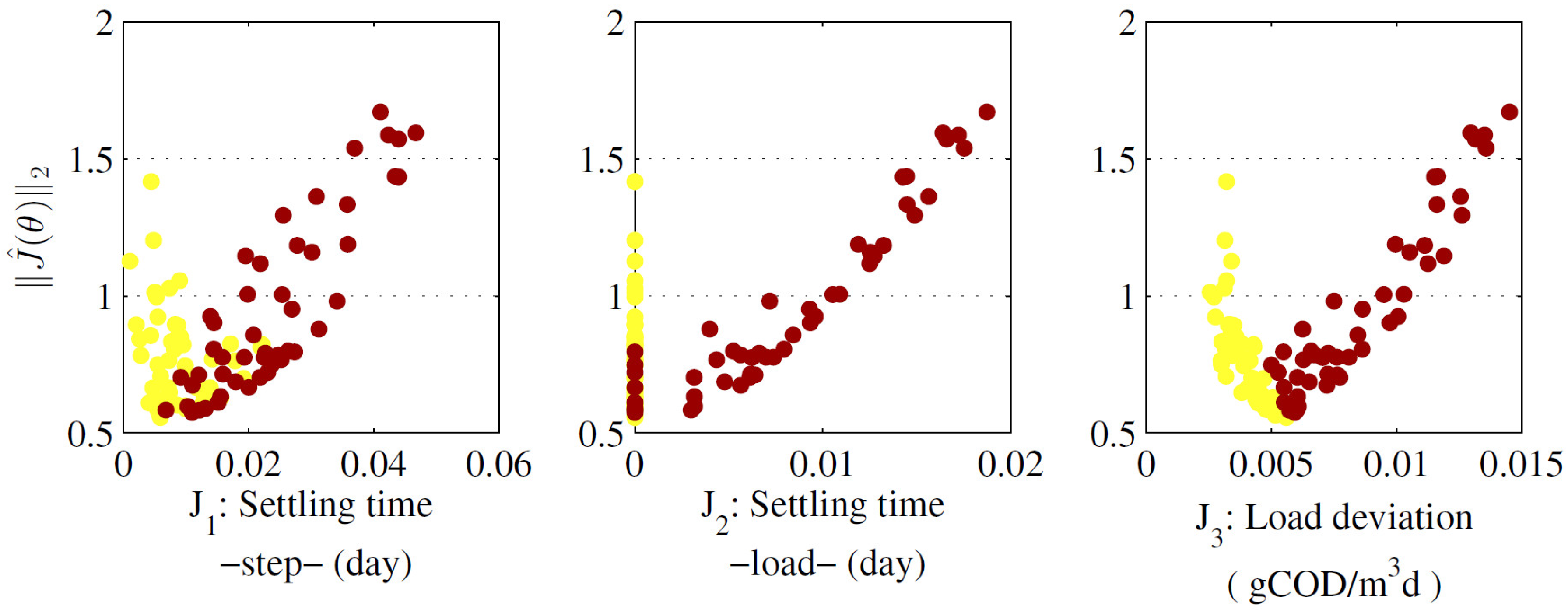
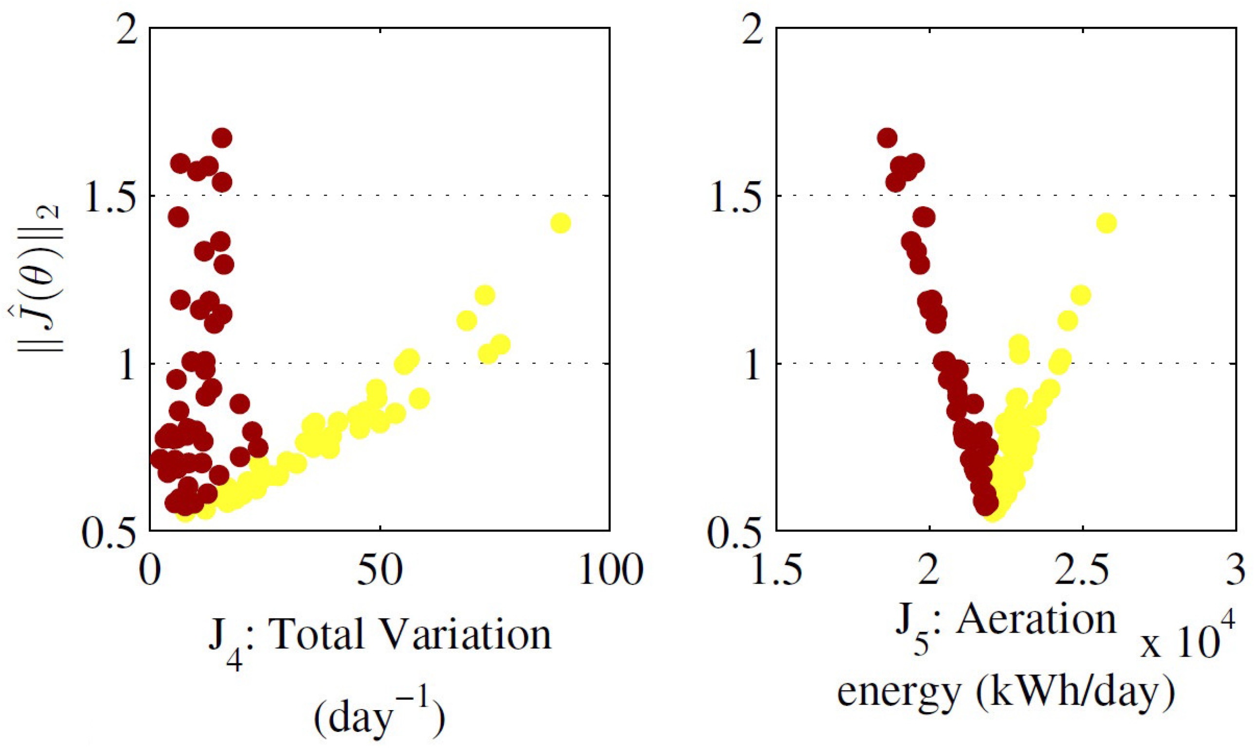
Results from optimisation process are depicted in Figure 1. Inflection point in design objective is used for further interpretability, in order to identify objective vectors with kWh/day and kWh/day. With such information is possible to track tendencies across subplots. For example, the lower the bigger , and . This means that a reduction on the aeration energy tends to worsen settling times and the load deviation capacity. In addition, it means that aeration energy and total variation of control action are correlated.
Using preferences stated in Table 5 and Table 6 and the TOPSIS method, three solutions have been selected for further control tests. Their time responses are depicted in Figure 2 when facing a setpoint change and a disturbance. As expected, none of such solutions is better than the others in an overall sense: each one has a unique trade-off. This approach might be used by a decision maker, in order to focus in a subset of approximated Pareto optimal solutions, to perform a final decision regarding the controller to implement. Next, we will actively use such methodologies and we will compare Pareto optimal solutions approximated in each case.
4.2. Case Study 2: Pollution Management in Water Distribution Systems
This case study is based on the hypothetical condensed example of the Bow River Valley, as presented in [37], and it follows the preliminary results that were presented in [38]. It deals with the pollution problem due to a cannery industry (Pierce-Hall Cannery), to two sources of municipal waste (Bowville and Plymton), with a park in the middle (Robin State Park). Water quality in the river is evaluated via dissolved oxygen concentration (DO). Quality of the effluent from the three treatment plants is measured with the biochemical oxygen demanding material (BOD) which is separated into carbonaceous and nitrogenous material (BODc and BODn respectively). The major aim of this example is to evaluate structural differences in the approximated Pareto fronts when using different policies in the pruning mechanism of the sp-MODEII.
The MOP under consideration has six design objectives:
- :
- DO level at Bowville (mg/L) (maximise).
- :
- DO level at Robin State Park (mg/L) (maximise).
- :
- DO level at Plymton (mg/L) (maximise).
- :
- Return on equity (%) (maximise).
- :
- Tax increment (Bowville) (minimise).
- :
- Tax increment (Plymton) (minimise).
Additionally, the DO at the state line (mg/L) is considered. Decision variables are the treatment levels of water discharge at the Pierce-Hall cannery, at Bowville and a Plymton, respectively. The constrained MOP for optimisation is as follows:
subject to
where
In Table 7 and Table 8 preferences stated are reported. Please note that congruence has been sought between them. That is, insignificant differences coincide with the tolerable interval, whilst significant differences coincide with the range from tolerability to highly desirability. This provides a guide in order to link both methods.
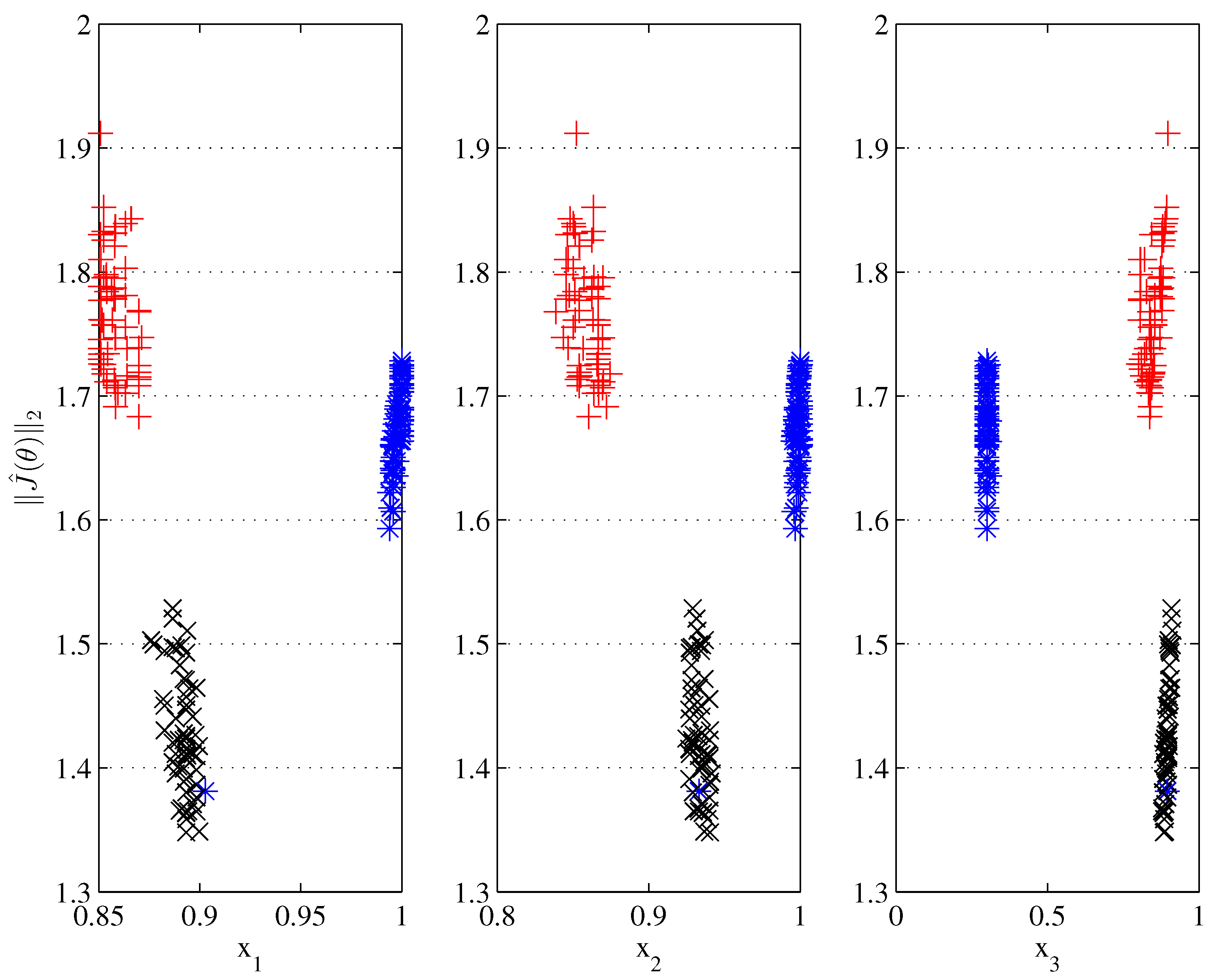
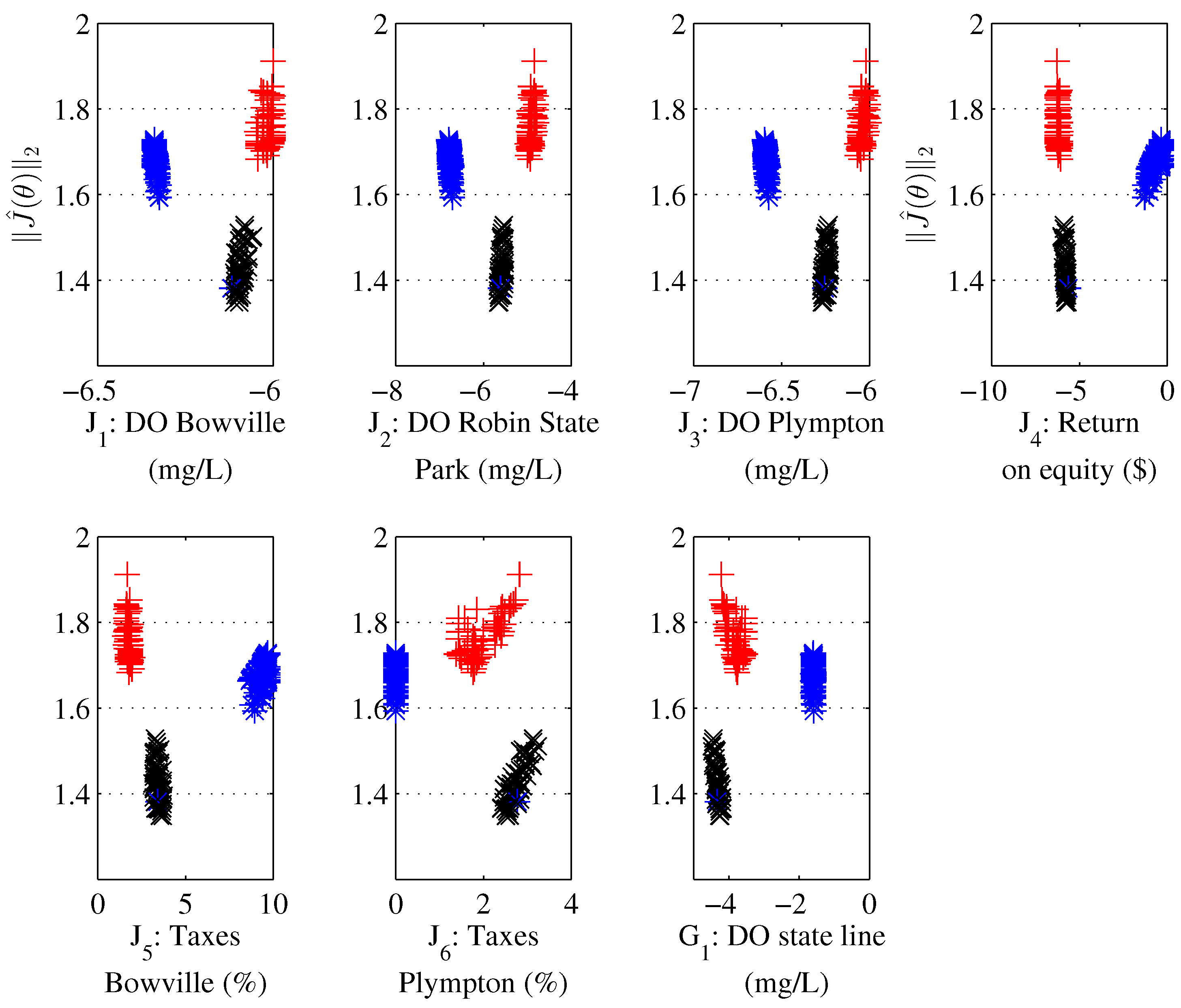
Pareto front and set approximations are depicted in Figure 3 and Figure 4, respectively. It is possible to appreciate that solutions are clustering towards different regions in the Pareto front, according to the information provided. TOPSIS solutions (black x) describe a cluster at the bottom of Level Diagrams; this is expected, given that the TOPSIS method seeks for a similarity with the utopian solution, which is also used to normalise the Pareto front approximation in Level Diagrams and calculate the selected norm. The next cluster correspond to the PROMETHEE II pruning (blue *) and the one on the upper region to Physical Programming (red +).
Main difference between TOPSIS and PP, is regarding design objective : the preference matrix states that a solution with is undesirable; that is the reason because the pruning mechanism tends to worsen the remainder design objectives, with the aim of improving . This does not mean that the TOPSIS mechanism gives worst results; it is important to remember that such mechanisms did not have any information about such undesirability. The same apply with the PROMETHEE II mechanism: provided information about (in) significant differences was helpful to evolve towards a desirable region in several design objectives, but fails in some of them.
In any case, the fact that, the bigger the norm, the more the information used by the pruning mechanism, reveals the philosophy behind multi-objective optimisation: it might be not enough to minimise a given norm, but to analyse/incorporate the trade-off analysis in a different way. In conclusion, the most the information provided by the designer, the most the accurate the algorithm to approximate a pertinent region in the objective space. Obviously this is in exchange of investing more time in stating the preferences a priori.
5. Conclusions
In this paper, we incorporated two additional mechanisms to handle designers’ preferences in multi-objective optimisation in the sp-MODEII algorithm. Such mechanisms are based on the TOPSIS and PROMETHEE methods, usually employed for multi-criteria analysis and decision making.
A comparison to handle designers’ preferences on two benchmarks dealing with water distribution systems was performed. On the one hand, it was shown that an analysis in such m-dimensional spaces with more than three design objectives is possible via specialised visualisation tool (Level Diagrams). On the other hand, the structural differences between different approaches to approximate a pertinent region of the Pareto front was also analysed.
In the latter case, the capacity to approximate a compact set focusing in the region of interest of the decision maker is evaluated. It was shown that the main structural difference among approaches (TOPSIS, PROMETHEE II, and Physical Programming) is the closeness of their clusters to an ideal solution, defined by the Pareto front approximation itself.
Further work will focus on using additional mechanisms to handle such preferences actively in the optimisation stage. Besides, merging two or more mechanisms might be an interesting idea to explore, in order to exploit synergies between different approaches.
Acknowledgments
This work is under the research initiative Multi-objective optimisation design (MOOD) procedures for engineering systems: Industrial applications, unmanned aerial systems and mechatronic devices, supported by the National Council of Scientific and Technological Development of Brazil (CNPq) through the grant PQ-2/304066/2016-8. This work is also supported by the Brazilian Federal Agency for Support and Evaluation of Graduate Education (CAPES) through the grant PROSUC/159063/2017-0.
Author Contributions
G.R.-M. and E.P.C.-A. conceived benchmark experiments; G.R.-M. and E.P.C.-A. performed benchmarks experiments; G.R.-M. and V.H.A.R. analysed the data; and G.R.-M. and V.H.A.R. wrote the paper. All authors read and approved the manuscript.
Conflicts of Interest
The authors declare no conflict of interest.
Abbreviations
The following abbreviations are used in this manuscript:
| EMO | Evolutionary Multi-Objective Optimisation |
| LD | Level Diagrams |
| MCDM | Multi-criteria Decision Making |
| MOP | Multi-Objective Problem |
| MOO | Multi-Objective Optimisation |
| PP | Physical Programming |
| WDS | Water Distribution System |
Appendix A. Background
A multi-objective problem (MOP) with m objectives, can be stated as follows [3]:
subject to:
where is defined as the decision vector with ; as the objective vector and , as the inequality and equality constraint vectors respectively; are the lower and the upper bounds in the decision space.
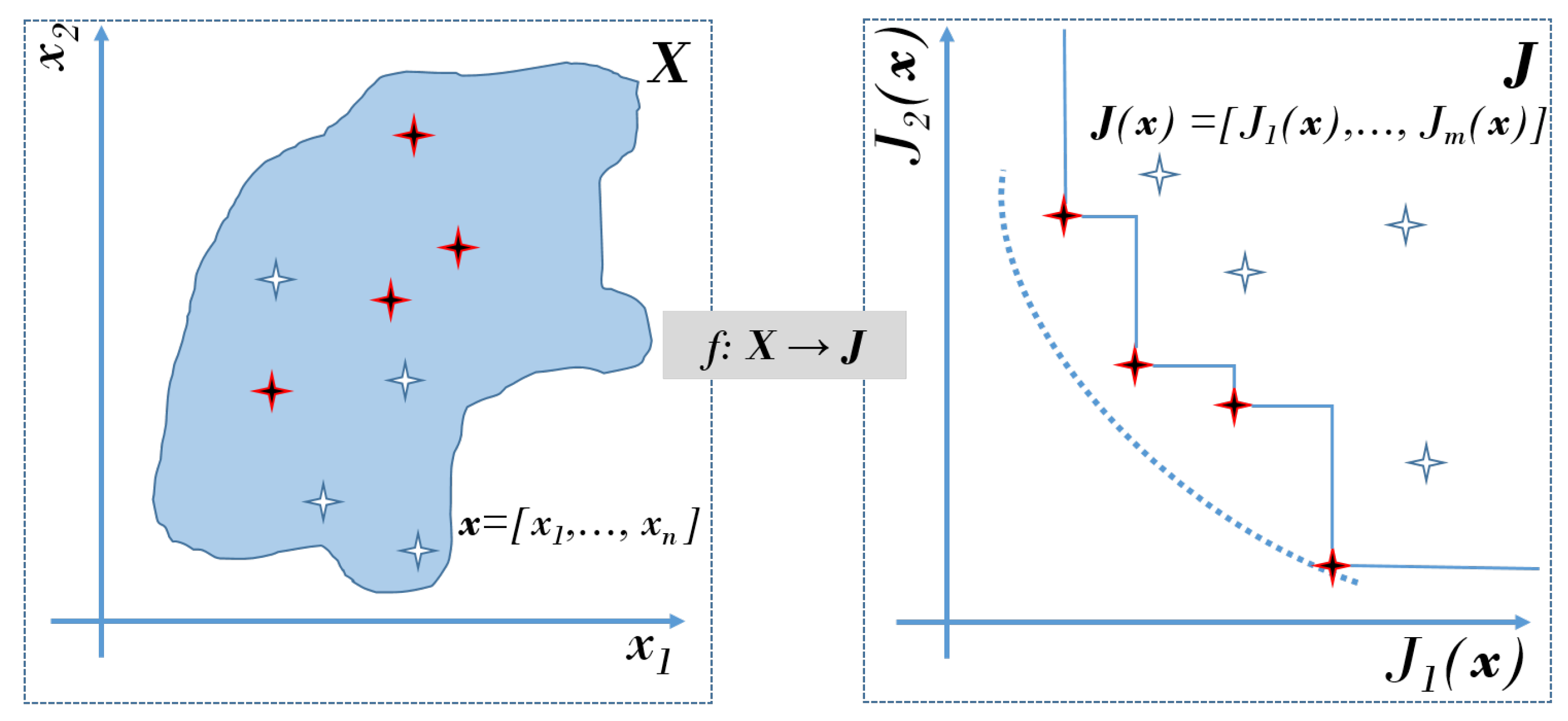
It has been noticed that there is not a single solution in MOPs, because there is not generally a better solution in all the objectives. Therefore, a set of solutions, the Pareto set, is defined. Each solution in the Pareto set defines an objective vector in the Pareto front (see Figure A1). All the solutions in the Pareto front are a set of Pareto optimal and non-dominated solutions:
- Pareto optimality [3]: An objective vector is Pareto optimal if there is not another objective vector such that for all and for at least one j, .
- Dominance: An objective vector is dominated by another objective vector if for all and for at least one j, . This is denoted as .
Figure A1.
Pareto optimality and dominance concepts for a min-min problem. Dark solutions is the subset of non-dominated solutions which approximates a Pareto front (right) and a Pareto set (left). Remainder solutios are dominated solutions, because it is possible to find at least one solution with better values in all design objectives (Source: [39]).
To successfully implement the multi-objective optimisation approach, three fundamental steps are required: the MOP definition, the multi-objective optimisation (MOO) process and the multi-criteria decision making (MCDM) stage. This integral and holistic process will be denoted hereafter as a multi-objective optimisation design (MOOD) procedure [40]. In the MOP statement, design objectives are defined, as well as decision variables (with their bounds) and constraints for feasibility or suitability; in the MOO the major aim is to calculate a useful Pareto front approximation via an algorithm; in the MCDM stage, an analysis of the approximated Pareto front and trade-offs is carried out according to a set of preferences, in order to select the final solution to implement.
There are different methodologies for MCDM and visualisation approaches [4,41]. In the case of the MOO process, special (or particular) circumstances might require additional mechanisms to deal successfully with a given MOP [40,42]. Some of them are listed below:
- Constrained optimisation. Results from the optimisation problem are not always feasible in a practical sense; therefore constraints must be incorporated in order to assure their feasibility.
- Many-objectives optimisation. If a MOP has more than 3 design objectives, it is considered a many-objectives optimisation problem. It is important to consider such a sub-classification, given that converge and diversity mechanisms might be in conflict.
- Computational expensive optimisation. Extensive or exhaustive simulations might be required in order to compute one or more design objectives requires.
- Multi-modal optimisation. It might happen that two or more decision vector points to the same objective vector.
For the MOO process, multi-objective evolutionary algorithms (MOEAs) have shown to be a useful tool for a wide range of engineering problems [43].
References
- Savic, D. Single-objective vs. multiobjective optimisation for integrated decision support. In Proceedings of the International Congress on Environmental Modelling and Software, Lugano, Switzerland, 24–27 June 2002. [Google Scholar]
- Mala-Jetmarova, H.; Sultanova, N.; Savic, D. Lost in optimisation of water distribution systems? A literature review of system operation. Environ. Model. Softw. 2017, 93, 209–254. [Google Scholar] [CrossRef]
- Miettinen, K. Nonlinear Multiobjective Optimization. In International Series in Operations Research and Management Science; Springer Science & Business Media: Berlkin, Germany, 1999; Volume 12. [Google Scholar]
- Tušar, T.; Filipič, B. Visualization of Pareto front approximations in evolutionary multiobjective optimization: A critical review and the prosection method. IEEE Trans. Evol. Comput. 2015, 19, 225–245. [Google Scholar] [CrossRef]
- Hwang, C.L.; Lai, Y.J.; Liu, T.Y. A new approach for multiple objective decision making. Comput. Oper. Res. 1993, 20, 889–899. [Google Scholar] [CrossRef]
- Messac, A. Physical programming: Effective optimization for computational design. AIAA J. 1996, 34, 149–158. [Google Scholar] [CrossRef]
- Behzadian, M.; Kazemzadeh, R.B.; Albadvi, A.; Aghdasi, M. PROMETHEE: A comprehensive literature review on methodologies and applications. Eur. J. Oper. Res. 2010, 200, 198–215. [Google Scholar] [CrossRef]
- Reynoso-Meza, G.; Sanchis, J.; Blasco, X.; García-Nieto, S. Multiobjective evolutionary algorithms for multivariable PI controller tuning. Appl. Soft Comput. 2014, 24, 341–362. [Google Scholar] [CrossRef]
- Reynoso-Meza, G. Controller Tuning by Means of Evolutionary Multiobjective Optimization: A Holistic Multiobjective Optimization Design Procedure. Ph.D. Thesis, Universitat Politècnica de València, València, Spain, 2014. [Google Scholar]
- Savic, D.A.; Walters, G.A.; Schwab, M. Multiobjective genetic algorithms for pump scheduling in water supply. In AISB International Workshop on Evolutionary Computing; Springer: Berlin, Germany, 1997; pp. 227–235. [Google Scholar]
- Sotelo, A.; Baran, B. Optimizacion de los costos de bombeo en sistemas de suministro de agua mediante un algoritmo evolutivo multiobjetivo combinado (Pumping cost optimization in water supply systems using a multi-objective evolutionary combined algorithm). In Proceedings of the XV Chilean Conference on Hydraulic Engineering, Concepción, Chile, 7–9 November 2001; pp. 337–347. [Google Scholar]
- Kelner, V.; Léonard, O. Optimal pump scheduling for water supply using genetic algorithms. In Proceedings of the Evolutionary Methods for Design, Optimization and Control with Applications to Industrial Problems (Eurogen 2003), Barcelona, Spain, 15–17 September 2003. [Google Scholar]
- Barán, B.; von Lücken, C.; Sotelo, A. Multi-objective pump scheduling optimisation using evolutionary strategies. Adv. Eng. Softw. 2005, 36, 39–47. [Google Scholar] [CrossRef]
- Lopez-Ibanez, M.; Prasad, T.D.; Paechter, B. Multi-objective optimisation of the pump scheduling problem using SPEA2. In Proceedings of the 2005 IEEE Congress on Evolutionary Computation, Edinburgh, UK, 2–5 September 2005; Volume 1, pp. 435–442. [Google Scholar]
- Odan, F.K.; Ribeiro Reis, L.F.; Kapelan, Z. Real-time multiobjective optimization of operation of water supply systems. J. Water Resour. Plan. Manag. 2015, 141, 04015011. [Google Scholar] [CrossRef]
- Stokes, C.S.; Maier, H.R.; Simpson, A.R. Water distribution system pumping operational greenhouse gas emissions minimization by considering time-dependent emissions factors. J. Water Resour. Plan. Manag. 2014, 141, 04014088. [Google Scholar] [CrossRef]
- Prasad, T.D.; Walters, G.; Savic, D. Booster disinfection of water supply networks: Multiobjective approach. J. Water Resour. Plan. Manag. 2004, 130, 367–376. [Google Scholar] [CrossRef]
- Kurek, W.; Brdys, M.A. Optimised allocation of chlorination stations by multi-objective genetic optimisation for quality control in drinking water distribution systems. IFAC Proc. Vol. 2006, 39, 232–237. [Google Scholar] [CrossRef]
- Ewald, G.; Kurek, W.; Brdys, M.A. Grid implementation of a parallel multiobjective genetic algorithm for optimized allocation of chlorination stations in drinking water distribution systems: Chojnice case study. IEEE Trans. Syst. Man Cybern. C Appl. Rev. 2008, 38, 497–509. [Google Scholar] [CrossRef]
- Alfonso, L.; Jonoski, A.; Solomatine, D. Multiobjective optimization of operational responses for contaminant flushing in water distribution networks. J. Water Resour. Plan. Manag. 2009, 136, 48–58. [Google Scholar] [CrossRef]
- Giustolisi, O.; Laucelli, D.; Berardi, L. Operational optimization: Water losses versus energy costs. J. Hydraul. Eng. 2012, 139, 410–423. [Google Scholar] [CrossRef]
- Kougias, I.P.; Theodossiou, N.P. Multiobjective pump scheduling optimization using harmony search algorithm (HSA) and polyphonic HSA. Water Resour. Manag. 2013, 27, 1249–1261. [Google Scholar] [CrossRef]
- Kurek, W.; Ostfeld, A. Multi-objective optimization of water quality, pumps operation, and storage sizing of water distribution systems. J. Environ. Manag. 2013, 115, 189–197. [Google Scholar] [CrossRef] [PubMed]
- Kurek, W.; Ostfeld, A. Multiobjective water distribution systems control of pumping cost, water quality, and storage-reliability constraints. J. Water Resour. Plan. Manag. 2012, 140, 184–193. [Google Scholar] [CrossRef]
- Mala-Jetmarova, H.; Barton, A.; Bagirov, A. Exploration of the trade-offs between water quality and pumping costs in optimal operation of regional multiquality water distribution systems. J. Water Resour. Plan. Manag. 2014, 141, 04014077. [Google Scholar] [CrossRef]
- Mala-Jetmarova, H.; Barton, A.; Bagirov, A. Impact of water-quality conditions in source reservoirs on the optimal operation of a regional multiquality water-distribution system. J. Water Resour. Plan. Manag. 2015, 141, 04015013. [Google Scholar] [CrossRef]
- Ishibuchi, H.; Tsukamoto, N.; Nojima, Y. Evolutionary many-objective optimization: A short review. In Proceedings of the IEEE Congress on Evolutionary Computation (CEC 2008), IEEE World Congress on Computational Intelligence, Hong Kong, China, 1–6 June 2008; pp. 2419–2426. [Google Scholar]
- Storn, R.; Price, K. Differential evolution–a simple and efficient heuristic for global optimization over continuous spaces. J. Glob. Optim. 1997, 11, 341–359. [Google Scholar] [CrossRef]
- Das, S.; Suganthan, P.N. Differential evolution: A survey of the state-of-the-art. IEEE Trans. Evol. Comput. 2011, 15, 4–31. [Google Scholar] [CrossRef]
- Das, S.; Mullick, S.S.; Suganthan, P.N. Recent advances in differential evolution–an updated survey. Swarm Evol. Comput. 2016, 27, 1–30. [Google Scholar] [CrossRef]
- Zhou, A.; Qu, B.Y.; Li, H.; Zhao, S.Z.; Suganthan, P.N.; Zhang, Q. Multiobjective evolutionary algorithms: A survey of the state of the art. Swarm Evol. Comput. 2011, 1, 32–49. [Google Scholar] [CrossRef]
- Reynoso-Meza, G.; Sanchis, J.; Blasco, X.; Martínez, M. Design of continuous controllers using a multiobjective differential evolution algorithm with spherical pruning. Appl. Evol. Comput. 2010, 6024, 532–541. [Google Scholar]
- Blasco, X.; Herrero, J.; Sanchis, J.; Martínez, M. A new graphical visualization of n-dimensional Pareto front for decision-making in multiobjective optimization. Inf. Sci. 2008, 178, 3908–3924. [Google Scholar] [CrossRef]
- Reynoso-Meza, G.; Blasco, X.; Sanchis, J.; Herrero, J.M. Comparison of design concepts in multi-criteria decision-making using level diagrams. Inf. Sci. 2013, 221, 124–141. [Google Scholar] [CrossRef]
- Blasco, X.; Reynoso-Meza, G.; Pérez, E.A.S.; Pérez, J.V.S. Asymmetric distances to improve n-dimensional Pareto fronts graphical analysis. Inf. Sci. 2016, 340, 228–249. [Google Scholar] [CrossRef]
- Holenda, B.; Domokos, E.; Redey, A.; Fazakas, J. Dissolved oxygen control of the activated sludge wastewater treatment process using model predictive control. Comput. Chem. Eng. 2008, 32, 1270–1278. [Google Scholar] [CrossRef]
- Monarchi, D.E.; Kisiel, C.C.; Duckstein, L. Interactive multiobjective programing in water resources: A case study. Water Resour. Res. 1973, 9, 837–850. [Google Scholar] [CrossRef]
- Reynoso-Meza, G.; Carreno-Alvarado, E.P.; Montalvo, I.; Izquierdo, J. Water pollution management with evolutionary multi-objective optimisation and preferences. In Proceedings of the Congress on Numerical Methods in Engineering CMN, Valencia, Spain, 3–5 July 2017. [Google Scholar]
- Reynoso-Meza, G.; Sanchis, J.; Blasco, X.; Martínez, M. Preference driven multi-objective optimization design procedure for industrial controller tuning. Inf. Sci. 2016, 339, 108–131. [Google Scholar] [CrossRef]
- Reynoso-Meza, G.; Sanchis, J.; Blasco, X.; Martínez, M. Controller tuning using evolutionary multi-objective optimisation: current trends and applications. Control Eng. Pract. 2014, 28, 58–73. [Google Scholar] [CrossRef]
- Lotov, A.V.; Miettinen, K. Visualizing the Pareto frontier. In Multiobjective Optimization; Springer: Berlin, Germany, 2008; pp. 213–243. [Google Scholar]
- Meza, G.R.; Ferragud, X.B.; Saez, J.S.; Durá, J.M.H. Tools for the Multiobjective Optimization Design Procedure. In Controller Tuning with Evolutionary Multiobjective Optimization; Springer: Berlin, Germany, 2017; pp. 59–88. [Google Scholar]
- Coello, C.A.C.; Lamont, G.B. Applications of Multi-Objective Evolutionary Algorithms; World Science: Singapore, 2004; Volume 1. [Google Scholar]
Figure 1.
Pareto front approximation for MOP I.


Figure 2.
Time response comparison among selected controllers for MOP I.
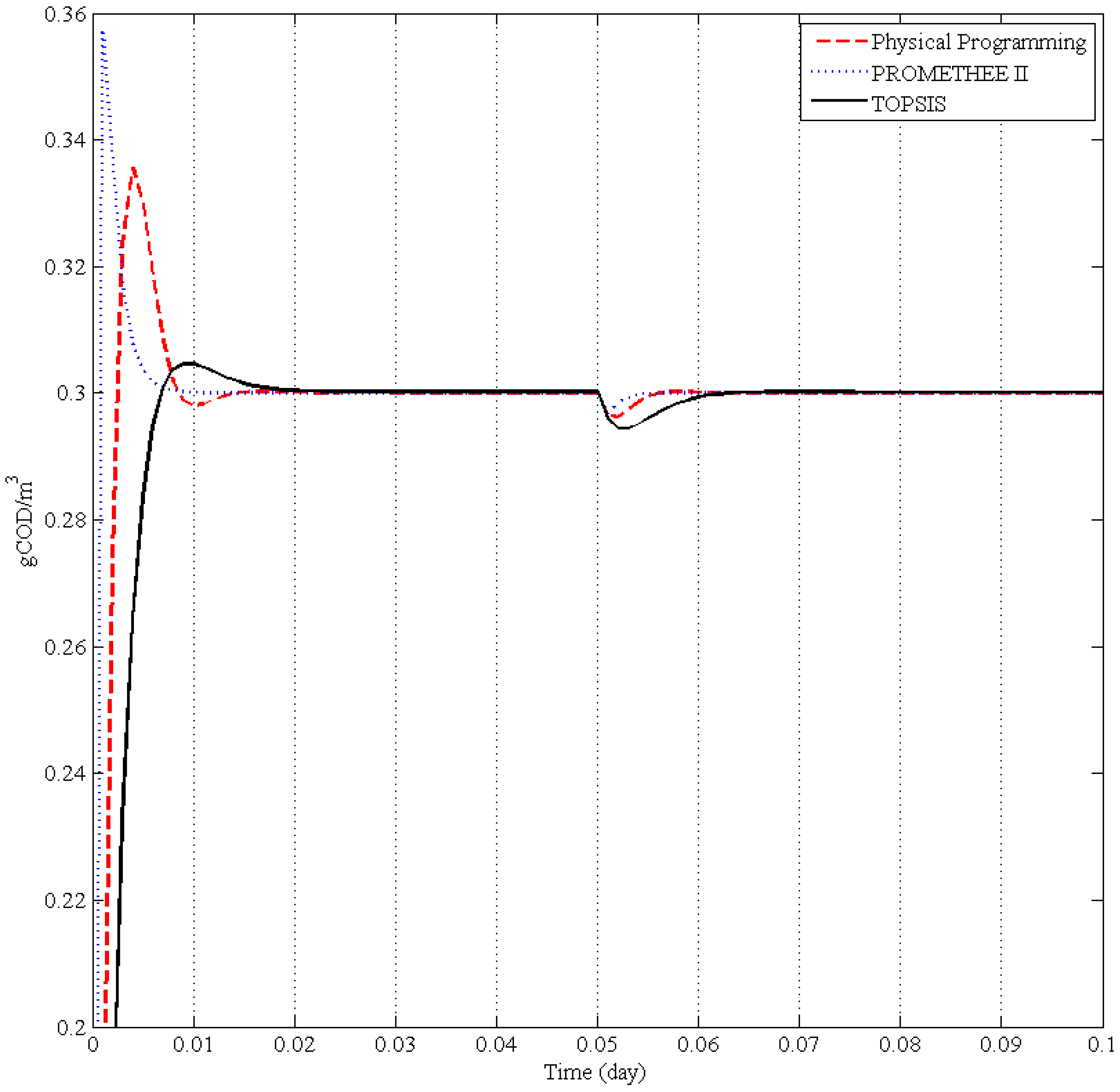
Figure 3.
Pareto front approximation for MOP II with preference pruning: PP (red +); PROMETHEE II (blue *) and TOPSIS (black x).
Figure 3.
Pareto front approximation for MOP II with preference pruning: PP (red +); PROMETHEE II (blue *) and TOPSIS (black x).

Figure 4.
Pareto set approximation for MOP II with preference pruning: PP (red +), PROMETHEE II (blue *) and TOPSIS (black x).
Figure 4.
Pareto set approximation for MOP II with preference pruning: PP (red +), PROMETHEE II (blue *) and TOPSIS (black x).

Table 1.
Summary of MOOD procedures for WDS design concept. refers to the number of objectives; to the number of sets of decision variables and , to the number of sets of inequality and equality constraints respectively.
Table 1.
Summary of MOOD procedures for WDS design concept. refers to the number of objectives; to the number of sets of decision variables and , to the number of sets of inequality and equality constraints respectively.
| Reference | MOP | MOO | MCDM | ||||
|---|---|---|---|---|---|---|---|
| Algorithm | Features | Plot | Insights | ||||
| Savic et al. [10] | 2 | 1 | (2, 1) | Hybrid GA | Local search | - | - |
| Sotelo and Baran [11] | 4 | 1 | (4, 0) | SPEA | - | Scatter plot | - |
| Kelner and Leonard [12] | 2 | 3 | (2, 2) | GAPS | Penalised tournament selection scheme | Scatter plot | - |
| Baran et al. [13] | 4 | 1 | (4, 0) | SPEA NSGA NSGA-II CNSGA NPGA MOGA | Comparison between algorithms | - | - |
| Lopez-Ibanez et al. [14] | 2 | 1 | (3, 1) | SPEA2 | Comparison between initial population generation methods | Scatter Plot | Attainment surfaces |
| Odan et al. [15] | 2 | 1 | (3, 1) | AMALGAM | Real-time | Scatter Plot | - |
| Stokes et al. [16] | 2 | 1 | (2, 0) | NSGA-II | - | Scatter Plot | Minimum objective values |
| Prasad et al. [17] | 2 | 2 | (3, 0) | NSGA-II | - | Scatter plot | - |
| Kurek and Brdys [18] | 3 | 2 | (5, 0) | NSGA-II | Problem specific modification | Scatter Plot | - |
| Ewald et al. [19] | 3 | 2 | (4, 0) | Distributed MOGA | Distributed application using grid computing | Scatter Plot | - |
| Alfonso et al. [20] | 3 | 1 | (2, 1) | NSGA-II | - | Scatter Plot | - |
| Giustolisi et al. [21] | 2 | 1 | (4, 1) | OPTIMOGA | - | Table | - |
| Kougias and Theodossiou [22] | 3 | 1 | (4, 0) | MO-HSA | - | Scatter Plot | - |
| Kurek and Ostfeld [23] | 3 | 3 | (3, 1) | SPEA2 | - | Scatter Plot | Utopian solution mechanism |
| Kurek and Ostfeld [24] | 2 | 2 | (3, 1) | SPEA2 | - | Scatter Plot | Most “balanced” solution |
| Mala-Jetmarova et al. [25] | 2 | 1 | (4, 0) | NSGA-II | - | Scatter Plot | - |
| Mala-Jetmarova et al. [26] | 3 | 1 | (4, 0) | NSGA-II | - | Scatter Plot | - |
Table 2.
Preference matrix M. Five preference ranges have been defined: highly desirable (HD), desirable (D), tolerable (T) undesirable (U) and highly undesirable (HU).
Table 2.
Preference matrix M. Five preference ranges have been defined: highly desirable (HD), desirable (D), tolerable (T) undesirable (U) and highly undesirable (HU).
| Preference Matrix | |||||||||||
|---|---|---|---|---|---|---|---|---|---|---|---|
| ← | HD | →← | D | →← | T | →← | U | →← | HU | → | |
| Objective | |||||||||||
| [-] | . | . | . | . | . | . | |||||
| … | |||||||||||
| [-] | . | . | . | . | . | . | |||||
Table 3.
Matrix with (in)significant differences. Significant (S) and Insignificant (I) differences for each design objectives are defined.
Table 3.
Matrix with (in)significant differences. Significant (S) and Insignificant (I) differences for each design objectives are defined.
| I/S Differences Matrix | ||
|---|---|---|
| Objective | I | S |
| [-] | . | . |
| … | ||
| [-] | . | . |
Table 4.
Input required for each preference mechanism.
| Method | Input |
|---|---|
| TOPSIS | Pareto front approximation. |
| PROMETHEE II | Pareto front approximation. |
| Significant/Insignificant differences. | |
| Physical Programming | Solution from the Pareto front approximation. |
| Information about the desirability limits. |
Table 5.
Preference matrix for MOP statement I. Five preference ranges have been defined: highly desirable (HD), desirable (D), tolerable (T) undesirable (U) and highly undesirable (HU).
Table 5.
Preference matrix for MOP statement I. Five preference ranges have been defined: highly desirable (HD), desirable (D), tolerable (T) undesirable (U) and highly undesirable (HU).
| Preference Matrix | |||||||||||
|---|---|---|---|---|---|---|---|---|---|---|---|
| Objective | ← | HD | →← | D | →← | T | →← | U | →← | HU | → |
| (day) | 0.03 | 0.04 | 0.05 | 0.06 | 0.07 | 0.08 | |||||
| (day) | 0.005 | 0.010 | 0.015 | 0.020 | 0.025 | 0.030 | |||||
| (/m day) | 0.000 | 0.005 | 0.010 | 0.0150 | 0.020 | 0.025 | |||||
| (day) | 20.00 | 30.00 | 40.00 | 50.00 | 60.00 | 70.00 | |||||
| (kWh/day) | 1.00 | 2.00 | 3.00 | 4.00 | 5.00 | 6.00 | |||||
Table 6.
Matrix with (in) significant differences for MOP statement I. Significant (S) and Insignificant (I) differences for each design objectives are defined.
Table 6.
Matrix with (in) significant differences for MOP statement I. Significant (S) and Insignificant (I) differences for each design objectives are defined.
| I/S Differences Matrix | ||
|---|---|---|
| Objective | I | S |
| (day) | 0.01 | 0.03 |
| (day) | 0.05 | 0.05 |
| (/m day) | 0.025 | 0.05 |
| (day) | 5.0 | 10.00 |
| (kWh/day) | 0.5 | 1.00 |
Table 7.
Matrix with (in)significant differences for MOP II statement. Significant (S) and Insignificant (I) differences for each design objectives are defined.
Table 7.
Matrix with (in)significant differences for MOP II statement. Significant (S) and Insignificant (I) differences for each design objectives are defined.
| I/S Differences Matrix | ||
|---|---|---|
| Objective | I | S |
| (mg/L) | 2.0 | 5.0 |
| (mg/L) | 2.0 | 5.0 |
| (mg/L) | 2.0 | 5.0 |
| ($) | 1.0 | 3.0 |
| (%) | 1.0 | 3.0 |
| (%) | 1.0 | 3.0 |
| (mg/L) | 0.5 | 1.5 |
Table 8.
Preference matrix for MOP II statement. Five preference ranges have been defined: highly desirable (HD), desirable (D), tolerable (T) undesirable (U) and highly undesirable (HU).
Table 8.
Preference matrix for MOP II statement. Five preference ranges have been defined: highly desirable (HD), desirable (D), tolerable (T) undesirable (U) and highly undesirable (HU).
| Preference Matrix | |||||||||||
|---|---|---|---|---|---|---|---|---|---|---|---|
| Objective | ← | HD | →← | D | →← | T | →← | U | →← | HU | → |
| (mg/L) | −9 | −8 | −6 | −4 | −2 | 0.0 | |||||
| (mg/L) | −9 | −8 | −6 | −4 | −2 | 0.0 | |||||
| (mg/L) | −9 | −8 | −6 | −4 | −2 | 0.0 | |||||
| ($) | −8 | −7 | −6 | −5 | −4 | −3 | |||||
| (%) | 0 | 1 | 2 | 3 | 4 | 5 | |||||
| (%) | 0 | 1 | 2 | 3 | 4 | 5 | |||||
| (mg/L) | −5 | −4.5 | −4 | −3.5 | −3.0 | −2.5 | |||||
© 2017 by the authors. Licensee MDPI, Basel, Switzerland. This article is an open access article distributed under the terms and conditions of the Creative Commons Attribution (CC BY) license (http://creativecommons.org/licenses/by/4.0/).
Share and Cite
MDPI and ACS Style
Reynoso-Meza, G.; Alves Ribeiro, V.H.; Carreño-Alvarado, E.P. A Comparison of Preference Handling Techniques in Multi-Objective Optimisation for Water Distribution Systems. Water 2017, 9, 996. https://doi.org/10.3390/w9120996
AMA Style
Reynoso-Meza G, Alves Ribeiro VH, Carreño-Alvarado EP. A Comparison of Preference Handling Techniques in Multi-Objective Optimisation for Water Distribution Systems. Water. 2017; 9(12):996. https://doi.org/10.3390/w9120996
Chicago/Turabian StyleReynoso-Meza, Gilberto, Victor Henrique Alves Ribeiro, and Elizabeth Pauline Carreño-Alvarado. 2017. "A Comparison of Preference Handling Techniques in Multi-Objective Optimisation for Water Distribution Systems" Water 9, no. 12: 996. https://doi.org/10.3390/w9120996
Note that from the first issue of 2016, this journal uses article numbers instead of page numbers. See further details here.