Article

Hydrological Modeling of Highly Glacierized Basins (Andes, Alps, and Central Asia)

by
Nina Omani
1,*,
Raghavan Srinivasan
2,
Raghupathy Karthikeyan
3 and
Patricia K. Smith
3
1
Former Graduate Research Assistant, Texas A&M University, College Station, TX 77843, USA
2
Spatial Sciences Laboratory, Department of Ecosystems Sciences and Management, Department of Biological and Agricultural Engineering, Texas A&M University, College Station, TX 77843, USA
3
Department of Biological and Agricultural Engineering, Texas A&M University, College Station, TX 77843, USA
*
Author to whom correspondence should be addressed.
Water 2017, 9(2), 111; https://doi.org/10.3390/w9020111
Submission received: 4 December 2016 / Revised: 26 January 2017 / Accepted: 3 February 2017 / Published: 10 February 2017

Abstract

:
The Soil and Water Assessment Tool (SWAT) was used to simulate five glacierized river basins that are global in coverage and vary in climate. The river basins included the Narayani (Nepal), Vakhsh (Central Asia), Rhone (Switzerland), Mendoza (Central Andes, Argentina), and Central Dry Andes (Chile), with a total area of 85,000 km2. A modified SWAT snow algorithm was applied in order to consider spatial variation of associated snowmelt/accumulation by elevation band across each subbasin. In previous studies, melt rates varied as a function of elevation because of an air temperature gradient while the snow parameters were constant throughout the entire basin. A major improvement of the new snow algorithm is the separation of the glaciers from seasonal snow based on their characteristics. Two SWAT snow algorithms were evaluated in simulation of monthly runoff from the glaciered watersheds: (1) the snow parameters are lumped (constant throughout the entire basin) and (2) the snow parameters are spatially variable based on elevation bands of a subbasin (modified snow algorithm). Applying the distributed SWAT snow algorithm improved the model performance in simulation of monthly runoff with snow-glacial regime, so that mean RSR decreased to 0.49 from 0.55 and NSE increased to 0.75 from 0.69. Improvement of model performance was negligible in simulations of monthly runoff from the basins with a monsoon runoff regime.

1. Introduction

The two basic snowmelt approaches generally used in hydrologic modeling are energy balance models and temperature-index models [1]. Temperature-index models are widely used in hydrologic studies because of the models’ performance and simplicity as well as the wide availability of temperature data [2,3,4].
In temperature-index based runoff models such as SWAT, melt rates only vary as a function of elevation, because of the air temperature gradient [5]. To overcome this drawback, a modified snow process was incorporated into SWAT in order to consider spatial variation of snowmelt/accumulation parameters by elevation band across subbasins. Previous studies using SWAT kept these parameters constant for an entire basin [6,7,8,9,10]. While this method was successful in simulation of snowmelt flow, simulation of runoff from glaciered watersheds demands a distributed model for distinguishing seasonal snow from glacier. The new approach allows for the separation of seasonal snowmelt from glaciers’ melt based on the spatial variability of associated melt parameters.
The SWAT model has been applied worldwide, and its hydrologic components have been successfully tested in cases where streamflow was predominantly generated from rainfall events [11,12,13,14,15]. The model less frequently has been applied in mountainous watersheds, and a few recent studies have been conducted to test and improve SWAT’s snow hydrology component. Fontaine et al. [16] incorporated the elevation bands method with SWAT’s original snowmelt algorithm (temperature-index model), which improved the Nash–Sutcliffe coefficient of monthly runoff simulation from −0.70 to 0.86 in the 4999-km2 Rocky Mountain Basin in Wyoming. Debele and Srinivasan [4] incorporated a modified version of SNOW17 [17] into SWAT and compared its performance with the temperature-index model in three watersheds (ranging from 22.28 to 7106.82 km2), the results of which showed that the temperature-index model performed better than the SNOW17 model. Debele et al. [18] incorporated the distributed process-based energy budget SNOWEB in the pixel and elevation band scales into SWAT and compared its performance with the temperature-index model. In this method, it was assumed that solar radiation varies not only with latitude and altitude of subbasins, which is applied in the current version of SWAT, but also with land surface inclinations (aspect and slope). The temperature-index based snowmelt computation method had overall Nash-Sutcliffe model efficiency coefficient ranging from 0.49 to 0.73 in simulation of monthly streamflow while the energy budget based approach had Nash-Sutcliffe efficiency coefficient ranging from 0.33 to 0.59. Zhang et al. [8] applied SNOW17 in SWAT at the pixel scale. The SWAT model with temperature-index plus elevation bands performed as well as the SWAT model with SNOW17. Rahman et al. [19] applied the modified temperature-index method [5] to simulate the runoff from fully and partially glaciated subbasins of the Rhone River Basin. The applied method showed improvement in simulated streamflow from the main outlet of the basin even though the snowmelt parameters were lumped across the basin.
Distributed, process-based energy budget models have been tested in SWAT, but we focused on another component of frequently used glacier/snowmelt models. A major difference between SWAT melt processes and the melt routine of hydroglacial models arises from the associated melt parameter distribution (melt factor). In previous studies using SWAT, associated snowmelt parameters were considered to be uniform within each subbasin, but in the hydroglacial models, melt factors are spatially variable in pixel or band scales. A common approach is to assign two different melt factors to ice and snow. This enables the user to treat seasonal snow and glaciers differently; melt factors are generally reported to be higher for glaciers and lower for snow [
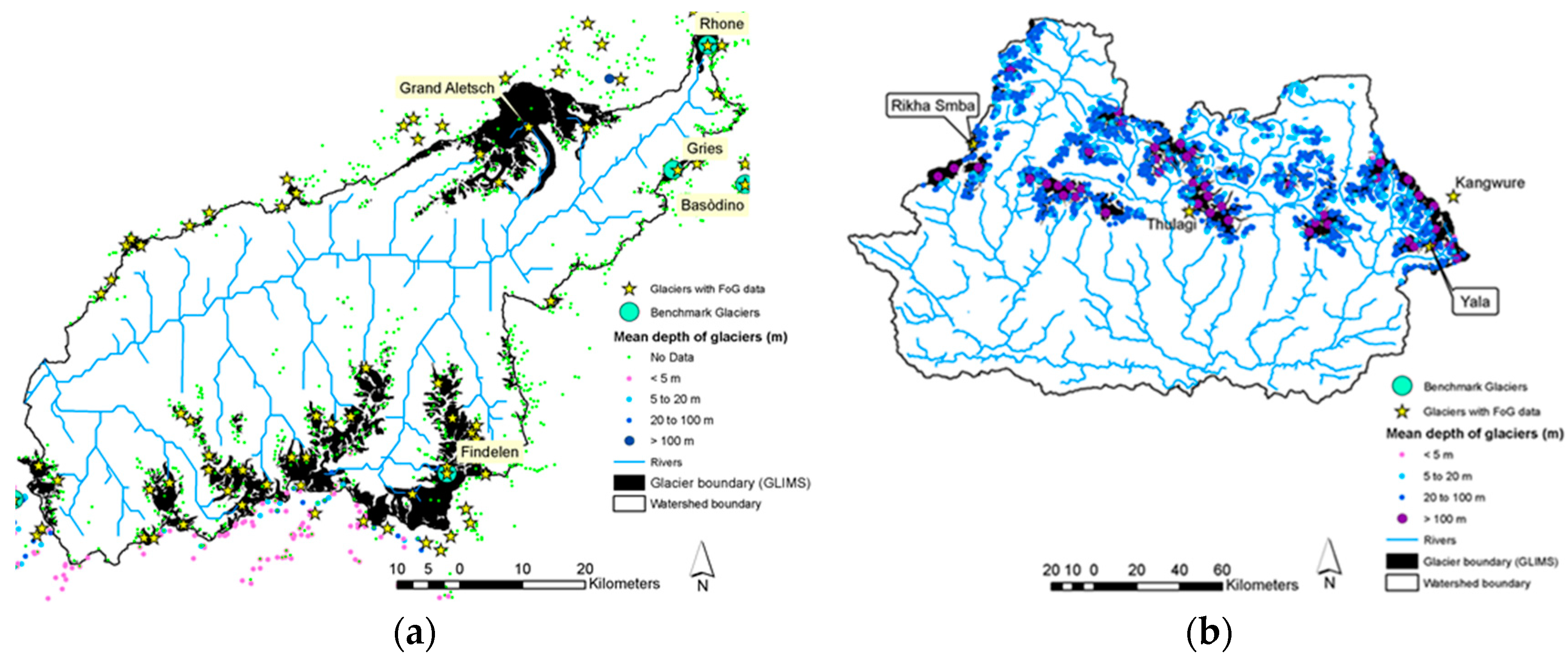
20]. The applied approach in this study separates seasonal snow from glaciers by setting the accumulation/melt parameters, including maximum and minimum melt factors, melt lag factor, melt temperature and snow fall temperature for the elevation bands of each subbasin. The details of the proposed approach are available at Omani et al. [
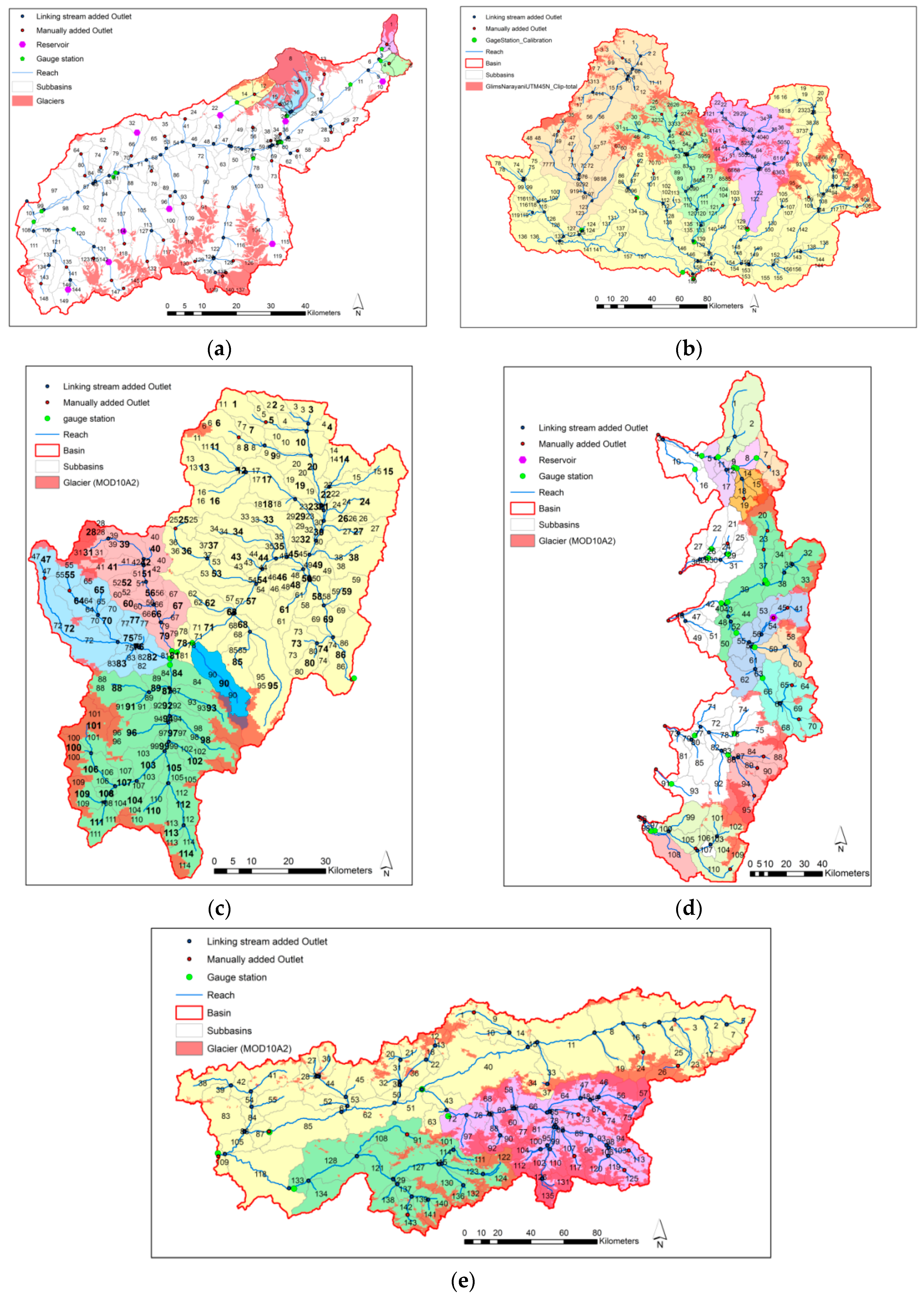
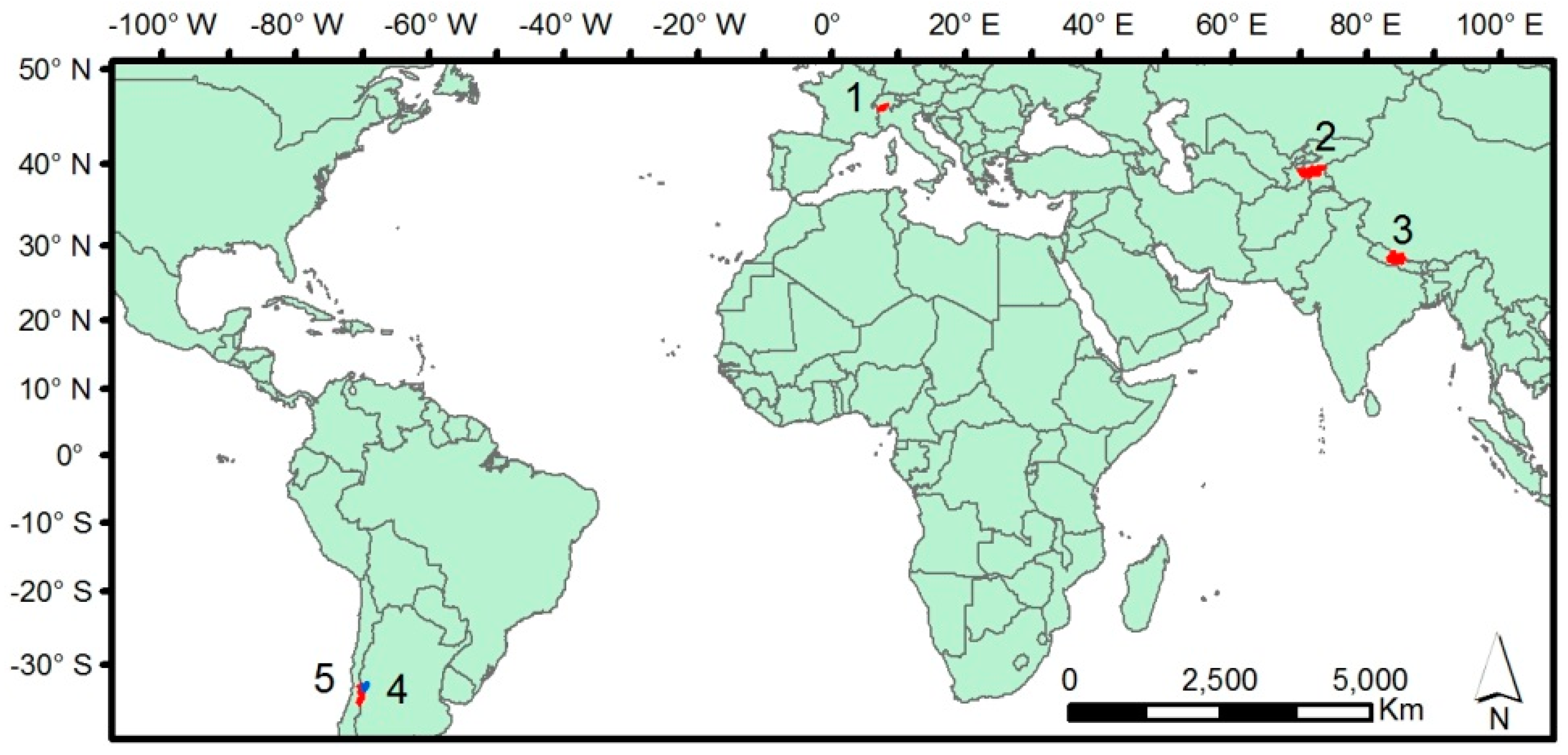
21] for three benchmark glaciers in Asia and Europe. The objective of this study was to extend the applied method to macro-scale river basins that are global in coverage and vary in climatic condition. Two snow process algorithms (lumped and distributed) were examined for their ability to simulate flow in five river basins that provide global assessment and feature contrasts in climatic conditions.

2. Materials and Methods

2.1. Study Watersheds

This study focuses on areas where climate variability has had a strong impact on highly glaciated areas. Five river basins with a total area of 85,000 km2, in the northern and southern hemispheres, for which sufficient hydrologic information is available were selected for this study. These river basins have different spatial scales and climatic situations, from extreme maritime to extreme continental climates. They include: Vakhsh in Tajikistan, Narayani in Nepal, Mendoza in Argentina, five individual glaciated watersheds in the central dry Andes of Chile, and Upper Rhone in Switzerland (Figure 1). Climate, hydrologic regime, soil, and land cover information for these watersheds can be found elsewhere [22].

2.2. Hydrologic Data

For this study, a 90-m resolution Global SRTM Digital Elevation Model contributed by USGS/NASA was used to describe topographic conditions such as slope and slope length, to create flow direction and accumulated flow, and to delineate watershed boundaries and channel networks [23]. Land use information was adopted from USGS Global Land-Cover Characteristics (GLCC). GLCC was developed using satellite data collected from 1992 to 1993 with 1 km spatial resolution for the entire globe [24]. Land use information can be found in Omani et al. (2016b). The soil properties dataset with 5 arc-minutes resolution (Ver. 1.2) was taken from ISRIC-WRS [25]. The major soil type in the upper areas of the river basins is Lithosols, which are very shallow and occur mainly on steep slopes, often with exposed rock debris. Weather data were obtained from the Climate Forecast System Reanalysis (CFSR) global meteorological dataset [26]. Global CFSR data are available going back to 1979 at a 38-km resolution. Daily discharge records for model calibration were collected from local hydrologic administrators and online databases (Table 1).

2.3. Model Simulation

This section focuses on glacier modelling in SWAT. More information about SWAT snow processes and theoretical details of the applied approach in this study can be found in Omani et al. [21].

2.3.1. Subbasin Delineation and HRU Definition

The watershed boundary of the river basins was determined using the SWAT interface automatic delineation procedure (Figure 2). Based on the thresholds selected, there were a total of 675 subbasins in the five river basins. SWAT further divides each subbasin into smaller areas called Hydrological Response Units (HRUs). There were a total of 9878 HRUs in the five river basins.

2.3.2. Initial Glacier Storage

The equilibrium line altitude (ELA) is a theoretical line where climatic mass balance is zero on average over a number of years and determines the boundary of the accumulation zone and ablation zone on a glacier. The ELA of a glacier is sometimes denoted ELA0 (the balanced-budget ELA). The ELA is determined by climate and the aspect of the glacier. It is not influenced by glacier dynamics, extent and hypsometry, and thus reveals a largely unfiltered climatic signal [27]. Therefore, it can be a representation of the lowest boundary of climatic glacierization [28].
In this study, it was assumed that the ELA0 represented the glacier boundary. The physical boundaries of glaciers were then corrected based on glacier inventory data, GLIMS glacier outlines and MODIS products for the glacier-free areas at elevations higher than the ELA0, and the areas climatically suited for glacier formation at altitudes lower than ELA0. Elevation bands below the ELA0 were considered to be seasonal snow cover regardless of glacial tongues extending into lower elevations. Debris-covered areas of glaciers, accumulated wind-blown snow, and small isolated glaciers with an area of 0.1 km2 or less were ignored when estimating the total glaciated area of the river basins. ELA0 values were obtained from the literature and are available in Table 2.
Glacier covered areas were extracted from the Global Land Ice Measurements from Space (GLIMS) [37,38] dataset and the World Glacier Inventory (WGI). If the GLIMS dataset did not completely cover the entire study area it was complimented with glaciated area by the Moderate Resolution Imaging Spectroradiometer (MODIS) maximum snow extent product (MOD10A2) with eight-day composites at 500-m resolution. The minimum snow cover area at the end of the melting season, from February 2002 to 2010, was considered to be the glacier/permanent snow cover area (Figure 3). The percentage of the glacier covered area of each river basin by each model, MODIS and GLIMS, is presented in Table 2. It is assumed that GLIMS glacier outlines represent the glacial extent at the end of the reference period as a starting point for the future simulations of glacial extent. The mean ice thickness in each elevation band was calculated by averaging the measured ice thickness values from the WGI. When no data were available for high elevations, ice thickness was assumed to be 1000 m water equivalent (m.w.e) (SNOEB = 999,999 mm H2O). Figure A1 and Figure A2 in Appendix A show the measurement locations of glacier depth and area from the WGI data inventory for the river basins.
Subbasins over 2000 m in altitude were divided into 10 elevation bands with 100-m to 200-m intervals, depending on the elevation range of the subbasin. Smaller elevation band intervals enable SWAT to model the glacier boundaries more accurately. It was assumed that the glacier boundary in a subbasin matched the lowest altitude of the elevation band if more than 50% of the elevation band area was covered by a glacier.

2.3.3. Model Calibration and Validation

The model was calibrated using monthly streamflow data at the gauge stations listed in Table 1, focusing on glaciated subbasins. The non-glaciated and snow-free gauged watersheds located at lowlands and glaciated subbasins with insufficient flow data, as well as dammed subbasins, were ignored in the model calibration. The model was validated using the monthly streamflow from the Rhone, Mendoza, and Chile for two periods: recent years from 2008 to 2010, and early years from 1982 to 1992. This was to confirm that the model works well for different periods. For the Vakhsh and Nepal River Basins, model validation periods were variable based on data availability.
Monthly calibration was performed using the SWAT Calibration and Uncertainty Program (SWAT-CUP) [39]. SWAT-CUP is a generic interface to provide a link between any automatic calibration/uncertainty or sensitivity program and SWAT. Sequential Uncertainty Fitting Version 2 (SUFI2) incorporated in SWAT-CUP allows for calibration and validation of the model at multiple gauging stations and multiple observed datasets simultaneously. SUFI2 calculates a weighted multi-component objective function (weighted summation of the square errors) based on simulated variables and observed time series of all gauged watersheds and then minimizes it by searching the Latin Hyperbolic [40] generated parameters for the best solution.
In order to perform automatic calibration by SUFI2, the initial parameter values and ranges were determined. A list of all snowfall/melt parameters and associated groundwater parameters and their ranges [23] are presented in Omani et al. [22]. Since most of the watersheds studied are glacier dominated and above the tree lines, the land use and soils in the upper catchment had little or no significant impact on hydrology such as evapotranspiration (ET). So, none of the land use or soil parameters were found to be sensitive in the model calibration process, which confirmed that the roles of these parameters are not important to the water budget. The groundwater delay (GW-DELAY) and baseflow recession constant (ALPHA-BF) were initially set for simulation of low flow during the winter months. The parameter values then were optimized during the automatic model calibration. The baseflow recession constant is directly proportional to groundwater flow response to changes in recharge.
The parameters were adjusted for the elevation bands above the ELA0 as an accumulation zone or glacier and below the ELA0 as an ablation zone with seasonal snow. The melt parameters for the elevation bands were adjusted in order to match the observed and simulated average monthly flow curves and then the parameters were optimized by automatic model calibration using SUFI2. Briefly, model calibration consisted of two main steps. First, parameters were automatically calibrated for an entire basin so that the snow parameters were uniform throughout the entire basin. In the next step, the results were improved by calibrating the model for snow parameters at the elevation band-subbasin scale. Model performance was tested in some of the smaller subbasins first and then extended into the larger subbasins to test the hypothesis that the hydrologic significance of meltwater may be negligible at the macro scale despite the presence of large glaciers in the headwaters area [41,42].
Calibration and validation were evaluated using the root mean square error-observations standard deviation ratio (RSR), the Nash–Sutcliffe Coefficient of Efficiency (NSE) [43] and the Percent Bias (PBIAS). RSR is a ratio of the RMSE and standard deviation of measured data. It ranges from the optimal value of 0 to a large positive value [44]. NSE indicates how well the plot of observed versus simulated data fits the 1:1 line. PBIAS measures the average tendency of the simulated data to be larger or smaller than their observed counterparts [45]. The optimal value of PBIAS is 0.0, with low values indicating accurate model simulation in term of magnitude.

3. Results and Discussion

Table 3, Table 4, Table 5, Table 6 and Table 7 show an average of adjusted values and range of the calibration parameters throughout the river basins for lumped and modified snow algorithms. The symbol “s” in the tables stands for glacier-free elevation bands or snowy elevation bands and “g” stands for glaciered elevation bands over the ELA0 altitudes. The calibration parameter values are averaged for the elevation bands and subbasins and the parameter range shows minimum and maximum parameter values based on elevation band-subbasin scale throughout the entire river basin. Mean SMFMX (Maximum melt factor) throughout all river basins is between 2.80 and 5.38, and 3.30 to 7.71, for snow and glacier, respectively. TIMP (Snow temperature lag factor) values are lower in the high elevation bands where the glaciers exist and range between 0.010 to 1.000 with average values between 0.025 for high elevation bands and 0.740 for low elevation bands. It can be seen from Table 3 that the average values for SMFMX and SMFMN (Minimum melt factor) for the Narayani River Basin are larger than the obtained values for Rhone River Basin (Table 4) as also was indicated by Kayastha et al. [46].
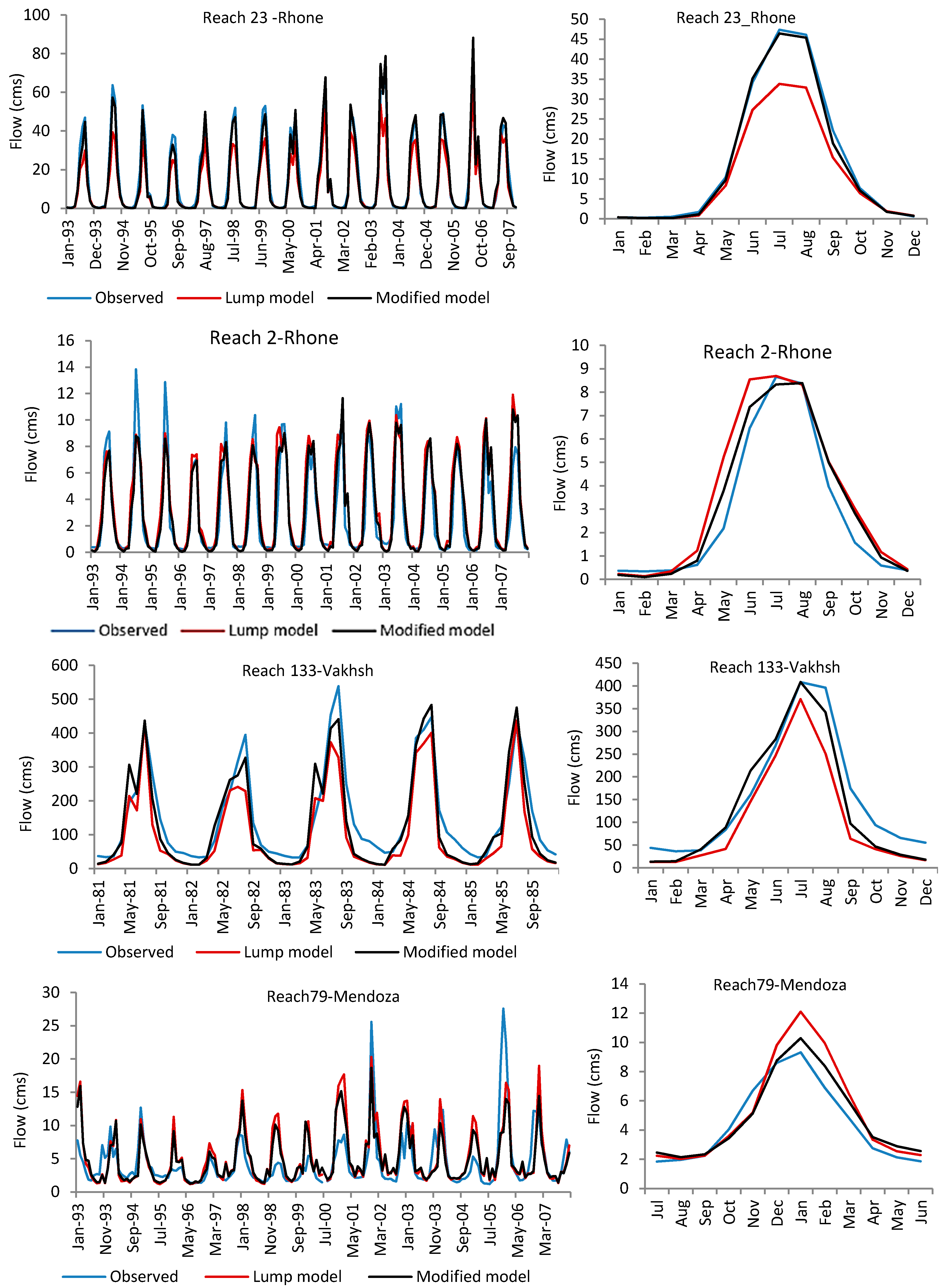
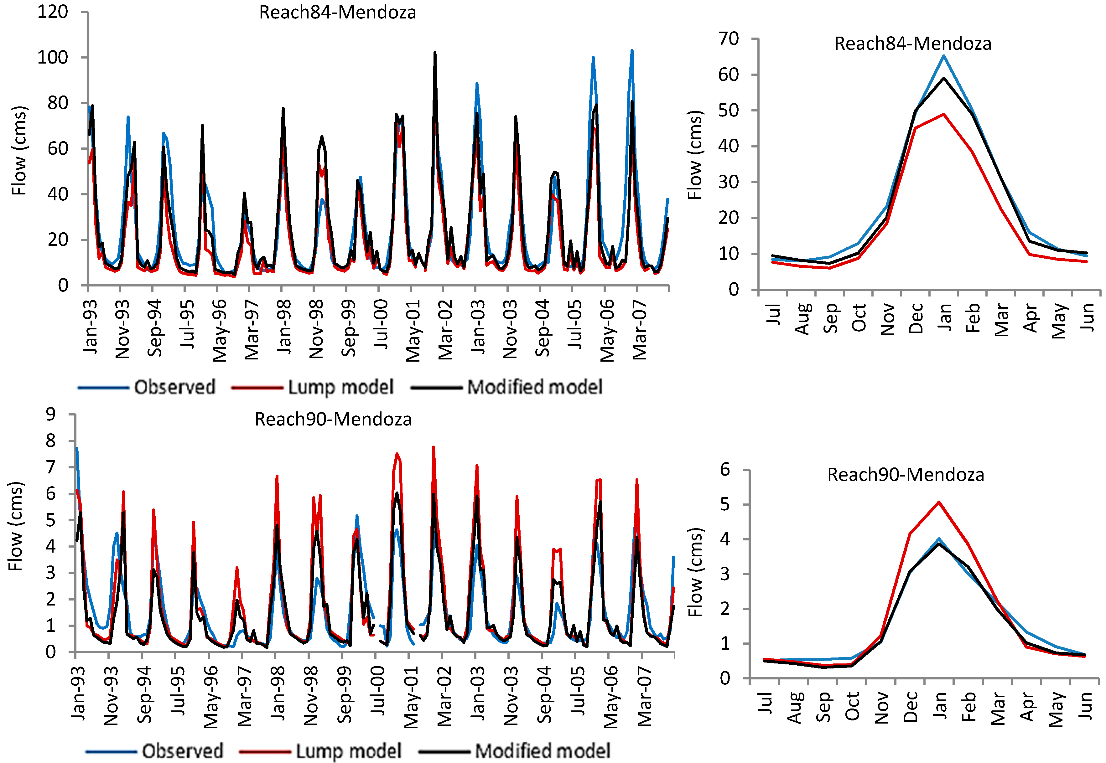
Figure 4 shows how the simulated monthly flow and mean monthly flow fit the observed mean monthly flow cycle using the modified algorithm for some of the selected reaches. This degree of accuracy in simulation of the seasonal pattern of monthly flow is only achievable by adjusting melt parameters based on elevation bands. As demonstrated in 
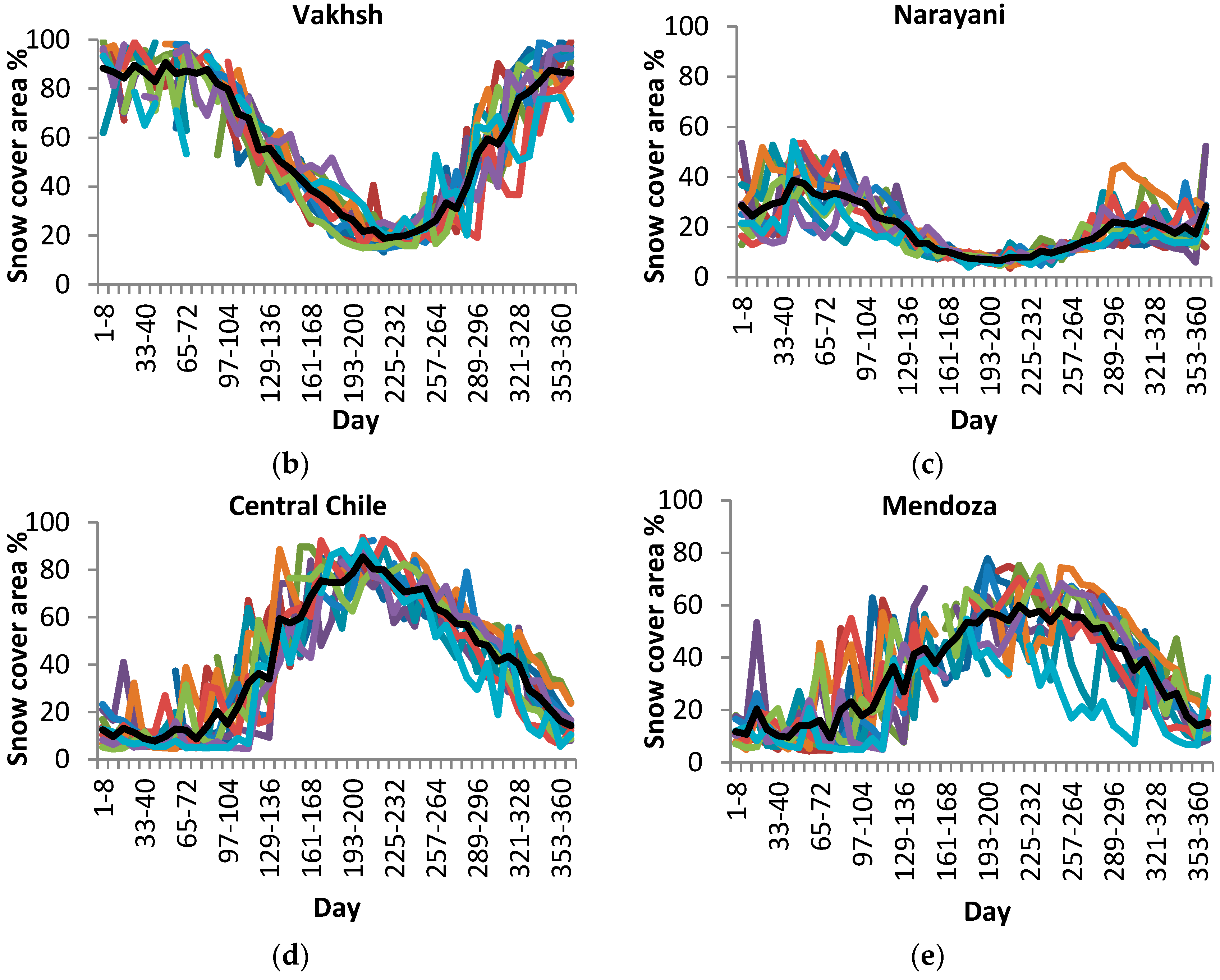
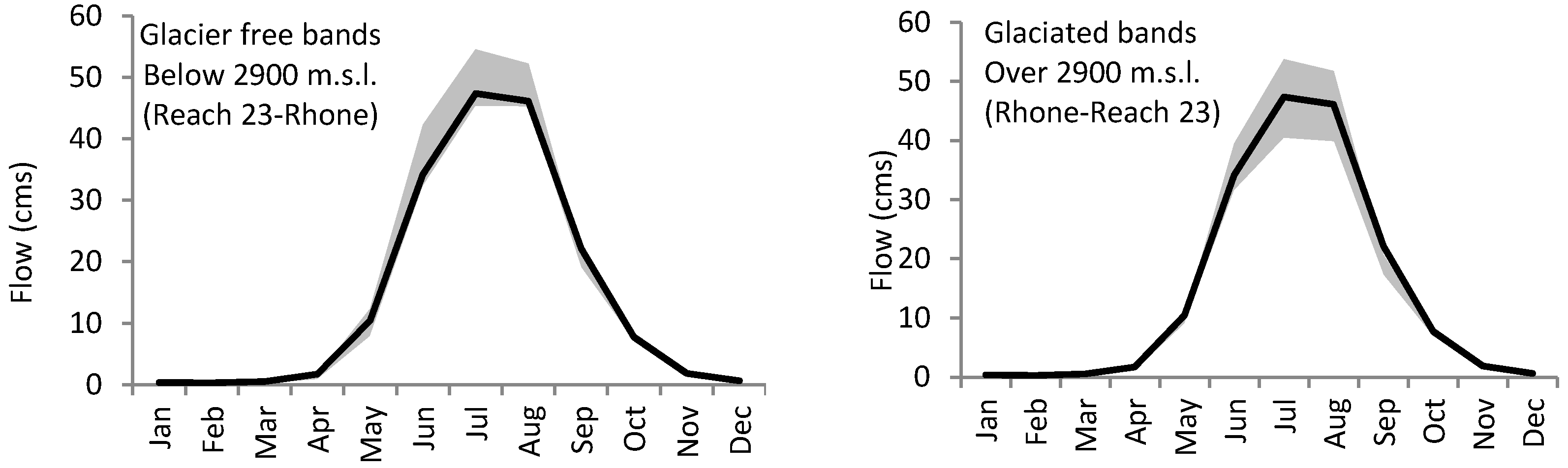
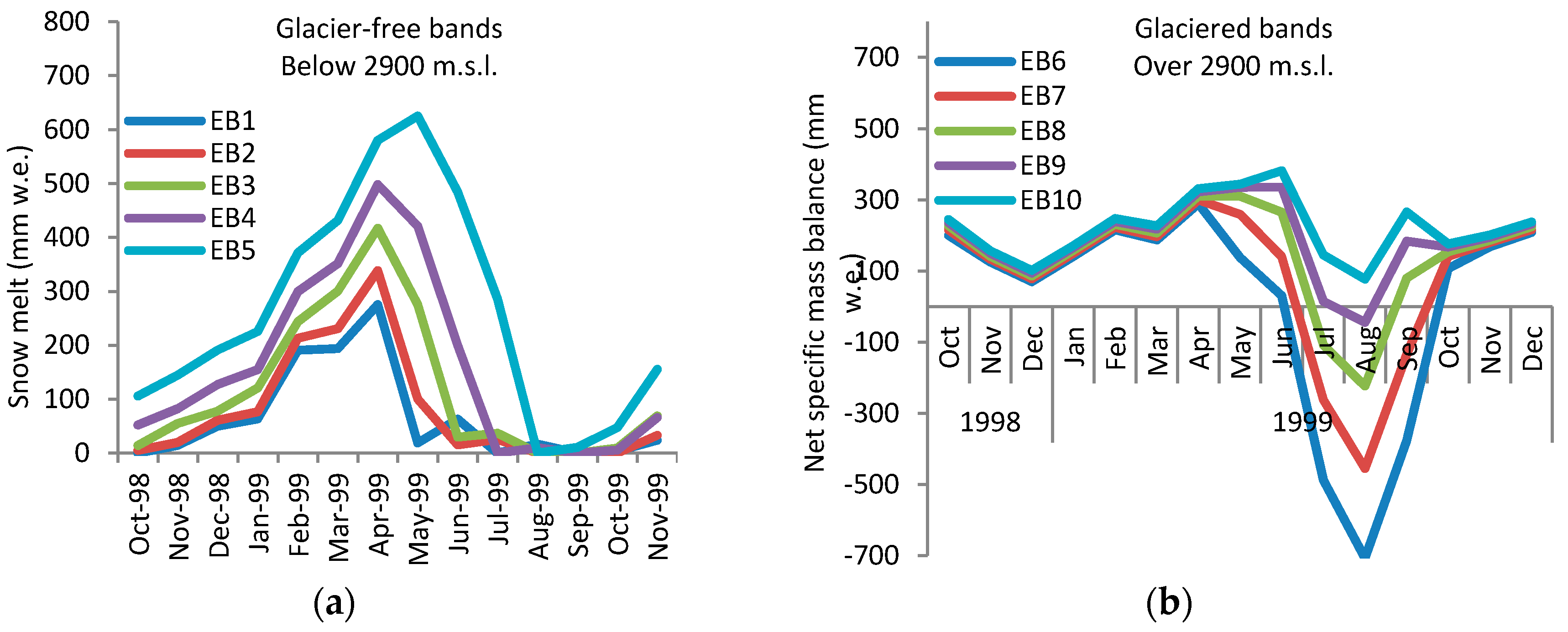
Figure 5, SMFMX changes in lower elevation bands had more influence on the rising limb of the flow curve, whereas the descending limb was more sensitive to SMFMX changes in the higher elevation bands (glaciered areas). This indicates that the late spring flow is under the influence of snowmelt at lower elevations and that late summer flow is controlled by glacier melt at higher elevations. This can also be investigated by analyzing the melting lag time at the elevation bands. Seasonal melting from October 1998 to October 1999 from each of the elevation bands of a typical subbasin with a wide range of elevations is presented in Figure 6a. Melting for glacier-free elevation bands with seasonal snow cover are presented in Figure 6b for high elevation bands with permanent snow cover or glacier. In Figure 6a, the snowpack in elevation bands 1, 2, 3, 4, and 5 has completely vanished by mid-August, whereas in Figure 6b the glacier ablation reaches its peak in August and continues through October. The melt was decreased at lower altitudes by decreasing the SMTMP (snow melt base temperature) and SFTMP (snowfall temperature) at lower elevation bands.
Calibration and validation results for all river basins are given in Table 8 and Table 9. In the watersheds with highly glaciered drainage areas (Reaches 2 and 23) in the Rhone River Basin, PBIAS was improved when the modified snow algorithm was used instead of lumping all of the parameters for entire watershed area Both RSR and NSE also were improved using the modified model, although the improvement is more significant in simulation of magnitude of flow. There is negligible improvement in the simulated flow from watersheds with small areas of glacier (Reach 4) when using the modified snow algorithm in comparison to the lumped snow algorithm.
For Narayani River Basin, PBIAS and NSE values in Table 8 reveal similar model performance by both lumped and modified snow algorithm methods, possibly as a result of the diminishing influence of glacier/snowmelt on runoff resulting from coincident summer monsoon precipitation in the Narayani River Basin. This monsoonal influence leads to accurate prediction of seasonal flow by rainfall–runoff models without explicitly considering the snow hydrology process. In Table 8, positive PBIAS in simulation of flow magnitude from all gauge stations (except Reach 96) means that the model has underpredicted the volume of flow. This systematic bias might be due to an underestimation of the NCEP reanalysis spring/summer precipitation (May–September) in the Narayani River basin of 20%.
The modified snow algorithm performed very well in simulation of monthly flow from the glaciered areas of the Vakhsh River Basin with RSR smaller than 0.5, PBIAS smaller than 10 percent and NSE greater than 0.70. Major difficulties in simulation of monthly flow from the Vakhsh River Basin were a lack of data for calibration and the low quality of the climate data, especially in the northern half of the river basin. The short calibration period of 2.5 years for Reach 72 was not long enough to capture the long-term variability of the monthly flow. The simulated mean monthly flow volume and cycle from the glaciated areas (drainage area to Reaches 72 and 133) by the modified snow algorithm during the summer months is in better agreement with the observed data in comparison to the mean monthly flow simulated using the lumped model for Reach 133 (Figure 4). At the main outlet (Reach 109), only the monthly flow variation shows improvement. Consequently, for an entire river basin it cannot be concluded that the modified model has better performance than the lumped model. Comparison between observed and simulated monthly flow from the main outlet of the basin during the validation period indicated that there was good agreement, verified by RSR, PBIAS, and NSE of 0.52, −8.15, and 0.73, respectively.
Among the gauged watersheds of the Mendoza River Basin, the drainage area of Reach 84 contains the largest area covered by glaciers. Subbasin 90 is a single gauged small subbasin, so it is a good example of the streamflow response to melt parameter distribution. There was a considerable improvement in the model performance when using the modified model instead of the lumped model in Reaches 79, 84, and 90. Figure 4 shows that the peaks simulated by the modified model match the observed peak flows. This level of accuracy is only achievable by adjusting the melt parameters for seasonal snow and permanent snow for each elevation band since the lumped model was not able to capture the peaks by calibrating the model for many different sets of melt parameters. Although the results from the modified model show significant improvement in highly glaciated areas and negligible improvement in less glaciated areas, the simulated monthly flow at the main outlet (Reach 86) does not show any improvement with the modified model. It can be seen in Table 8 that the model performance in simulation of downstream flow (e.g., Outlet 86 in the Mendoza River basin) declines when applying the modified snow algorithm. The new approach enabled calibration of the model versus the flow from upland catchments and optimization of the simulation results by adjusting the parameters separately for subbasin/elevation bands, while in the lump method the parameters were adjusted in order to get the reasonable result and were not necessarily the best at the gauged streams. It seems that the parameter value optimization for upland basins negatively affects the downstream flow in comparison to the lump parameter adjustment method. In other words, factors other than snowmelt could affect the downstream flow, and further model setup and parameter adjustment (groundwater, plant growth and soil moisture parameters, etc.) are necessary for lowlands and flat areas, which were out of the scope of this study. Another reason for declining the accuracy of downstream flow simulation could be the use of inaccurate reanalysis precipitation data. While snowfall/melt is the dominant hydrologic process in dry highlands (highland areas of Mendoza are very dry), flow is less affected by precipitation events, and snow parameter adjustment improves the flow simulation considerably. In lowlands, where the rainfall-runoff model is dominant, the flow is directly under the influence of precipitation events and any problem in input precipitation data could directly decline the accuracy of downstream flow simulation. So, when the results for snowy basins show improvement, flow in lowland areas may not necessarily improve. Comparisons between observed and simulated monthly streamflow during the validation period indicate range of model performances from good to unsatisfactory.
Comparisons between observed and simulated monthly flow from Chilean river basins during the calibration period indicate poor to satisfactory simulation. The RSR and NSE values are generally lower than those values obtained in simulation of monthly flows from the other river basins in this study. Winter precipitation (October to March) inter-annual variability in the Andes is linked to ENSO (El Niño–Southern Oscillation) events and consequently reveals a more complex response of streamflow [47], which may explain poor model performance in simulation of seasonal flow variability in the Mendoza River Basin and the Chilean river basins in the dry central Andes.

4. Conclusions

Treating the glaciered and un-glaciered areas in the watersheds separately improved SWAT model performance significantly in simulation of volume and variation of runoff in glaciered areas. Spatial and temporal variations of melt rates mainly depend on the spatial and temporal variations of melt factors in hydro-glacial models. While temporal variations of melt factors have been considered in the SWAT model in the past, there has been no consideration of spatial variations in melt factors and lag time factor, which are directly influenced by surface type (snow and ice). In this study, these spatial variations were specifically taken into account.
Model performance using the snow algorithms also depends on the climate of a river basin. Significance of melt water may be negligible in watersheds where the melt season coincides with monsoon precipitation, resulting in no significant difference in the simulation results from the two melt algorithms when monsoons were a factor. For the river basins in the central Andes, applying the modified distributed snow algorithm considerably improved the model performance in simulation of runoff volume in comparison with the lumped snow algorithm, while variation of runoff did not show any improvement. This may be due to high inter-annual and annual variability of flow in these regions, which are more dominated by rainfall-runoff relationships than snowmelt. We can conclude that considering the spatial variations of associated melt parameters significantly improves the SWAT performance in simulation of runoff volume and its seasonal variation in highly glaciated river basins.
While distributed process-based energy budget models have been tested in the SWAT model, no studies have been done to incorporate enhanced temperature-index models into SWAT. Incorporation of an enhanced temperature-index model into the modified snow algorithm of SWAT should be an objective of future studies on enhancing the SWAT snow hydrologic process. The modified snow algorithm did not enhance SWAT model performance in simulation of the streamflow at the main outlet of the river basins. Based on this, one might be tempted to draw the conclusion that at the macro scale the lumped model is preferable to the distributed model. This, however, requires further investigation into modeling such hydrologic processes as glacier surface mass balance and transient snow line altitude. Therefore, it is suggested that the model not only be calibrated using runoff but also be calibrated against the individual snow hydrology components.

Author Contributions

For research articles with several authors, a short paragraph specifying their individual contributions must be provided. The following statements should be used “Nina Omani and Raghavan Srinivasan conceived and designed this study and prepared the initial manuscript; Raghavan Srinivasan, Raghupathy Karthikeyan and Patricia K. Smith supervised reporting and manuscript preparation. All the authors finalized the research article together.”

Conflicts of Interest

The authors declare no conflict of interest.

Appendix A

Figure A1. Glacier snow depth and area across the (a) Rhone and (b) Narayani river basins extracted from the GLIMS glacier outlines. Green dots show locations of glaciers with no depth information.
Water 09 00111 g007
Figure A2. Glacier snow depth and area across the (a) Mendoza, (b) central Chile, and (c) Vakhsh river basins. Minimum snow cover area from MOD10A2 at the end of the melting season from February 2002 to 2010 was considered as glacier or permanent snow cover for Mendoza, central Chile, and part of the Vakhsh basin. Green dots show locations of glaciers with no depth information.
Water 09 00111 g008aWater 09 00111 g008b

References

  1. Anderson, E.A. National Weather Service River Forecast System-Snow Accumulation and Ablation Model; NOAA Technical Memorandum NWS-HYDRO-17; National Oceanographic and Atmospheric Administration Silver Springs Md: Washington, DC, USA, 1973.
  2. Moor, R.D. Application of a Conceptual Streamflow Model in a Glacierized Drainage Basin. J. Hydrol. 1993, 150, 151–168. [Google Scholar] [CrossRef]
  3. Schaper, J.; Seidel, K.; Martinec, J. Precision Snow Cover and Glacier Mapping for Runoff Modelling in a High Altitude Alpine Basin. In Remote Sensing and Hydrology, Proceedings of the Santa Fe Symposium 2000; International Association of Hydrological Sciences: Wallingford, CT, USA, 2000; pp. 105–111. [Google Scholar]
  4. Debele, B.; Srinivasan, R. Comparison of the Performances of Temperature-Index and Process-Based Energy Budget Snowmelt Estimation Approaches in the SWAT Model; Texas A&M University Spatial Sciences Laboratory: College Station, TX, USA, 2005; p. 40. [Google Scholar]
  5. Hock, R. Temperature Index Melt Modelling in Mountain Areas. J. Hydrol. 2003, 282, 104–115. [Google Scholar] [CrossRef]
  6. Wang, X.; Melesse, A.M. Evaluation of the SWAT Model’s Snowmelt Hydrology in a Northwestern Minnesota Watershed. Trans. ASAE 2005, 48, 1359–1376. [Google Scholar] [CrossRef]
  7. Ahl, R.S.; Woods, S.W.; Zuuring, H.R. Hydrologic Calibration and Validation of SWAT in a Snow-Dominated Rocky Mountain Watershed Montana U.S.A. J. Am. Water Resour. Assoc. 2008, 44, 1411–1430. [Google Scholar] [CrossRef]
  8. Zhang, X.S.; Srinivasan, R.; Debele, B.; Hao, F.H. Runoff Simulation of the Headwaters of the Yellow River Using the SWAT Model with Three Snowmelt Algorithms. J. Am. Water Resour. Assoc. 2008, 44, 48–61. [Google Scholar] [CrossRef]
  9. Stehr, A.; Debels, P.; Arumi, J.L.; Romero, F.; Alcayaga, H. Combining the Soil and Water Assessment Tool (SWAT) and MODIS Imagery to Estimate Monthly Flows in a Data-Scarce Chilean Andean Basin. Hydrol. Sci. J. 2009, 54, 1053–1067. [Google Scholar] [CrossRef]
  10. Pradhanang, S.M.; Anandhi, A.; Mukundan, R.; Zion, M.S.; Pierson, D.C.; Schneiderman, E.M.; Matonse, A.; Feri, A. Application of SWAT Model to Assess Snowpack Development and Streamflow in the Cannonsville Watershed New York USA. Hydrol. Process. 2011, 25, 3268–3277. [Google Scholar] [CrossRef]
  11. Srinivasan, R.; Ramanarayanan, T.S.; Arnold, J.G.; Bednarz, S.T. Large Area Hydrologic Modeling and Assessment: Part II. Model Application. J. Am. Water Resour. Assoc. 1998, 34, 91–101. [Google Scholar] [CrossRef]
  12. Arnold, J.G.; Muttiah, R.S.; Srinivasan, R.; Allen, P.M. Regional Estimation of Base Flow and Groundwater Recharge in the Upper Mississippi Basin. J. Hydrol. 2000, 227, 21–40. [Google Scholar] [CrossRef]
  13. Arnold, J.G.; Srinivasan, R.; Muttiah, R.S.; Allen, P.M.; Walker, C. Continental Scale Simulation of the Hydrologic Balance. J. Am. Water Resour. Assoc. 1999, 35, 1037–1052. [Google Scholar] [CrossRef]
  14. Arnold, J.G.; Srinivasan, R.; Muttiah, R.S.; Williams, J.R. Large Area Hydrologic Modeling and Assessment: Part I. Model Development. J. Am. Water Resour. Assoc. 1998, 34, 73–89. [Google Scholar] [CrossRef]
  15. Di Luzio, M.; Srinivasan, R.; Arnold, J.G. Integration of Watershed Tools and SWAT Model into BASINS. J. Am. Water Resour. Assoc. 2002, 38, 1127–1141. [Google Scholar] [CrossRef]
  16. Fontaine, T.A.; Cruickshank, T.S.; Arnold, J.G.; Hotchkiss, R.H. Development of a Snowfall-Snowmelt Routine for Mountainous Terrain for the Soil Water Assessment Tool (SWAT). J. Hydrol. 2002, 262, 209–223. [Google Scholar] [CrossRef]
  17. Anderson, E.A. A Point Energy and Mass Balance Model of a Snow Cover; NOAA Technical Report NWS 19; National Oceanic and Atmospheric Administration Silver Springs Md: Washington, DC, USA, 1976; 150p.
  18. Debele, B.; Srinivasan, R.; Gosain, A.K. Comparison of Process-Based and Temperature-Index Snowmelt Modeling in SWAT. Water Resour. Manag. 2010, 24, 1065–1088. [Google Scholar] [CrossRef]
  19. Rahman, K.; Maringanti, C.; Beniston, M.; Widmer, F.; Abbaspour, K.; Lehmann, A. Streamflow Modeling in a Highly Managed Mountainous Glacier Watershed using SWAT: The Upper Rhone River Watershed Case in Switzerland. Water Resour. Manag. 2013, 27, 323–339. [Google Scholar] [CrossRef]
  20. Braithwaite, R.J. Temperature and Precipitation Climate at the Equilibrium-Line Altitude of Glaciers Expressed by the Degree-Day Factor for Melting Snow. J. Glaciol. 2008, 54, 437–444. [Google Scholar] [CrossRef]
  21. Omani, N.; Srinivasan, R.; Smith, P.K.; Karthikeyan, R. Glacier mass balance simulation using SWAT distributed snow algorithm. Hydrol. Sci. J. 2016. [Google Scholar] [CrossRef]
  22. Omani, N.; Srinivasan, R.; Karthikeyan, R.; Venkatta, K.; Smith, P.K. Impacts of climate change on the glacier melt runoff from five river basins. Trans. ASABE 2016, 59. [Google Scholar] [CrossRef]
  23. Neitsch, S.L.; Arnold, J.G.; Kiniry, J.R.; Williams, J.R. Soil and Water Assessment Tool Theoretical Documentation Version 2009; Texas Water Ressources Institute Technical Report 406; Texas A&M University System: College Station, TX, USA, 2011. [Google Scholar]
  24. Brown, J.F.; Loveland, T.R.; Merchant, J.W.; Reed, B.C.; Ohlen, D.O. Using Multisource Data in Global Land Cover Characteristics: Concepts Requirements and Methods. Photogramm. Eng. Remote Sens. 1993, 59, 977–987. [Google Scholar]
  25. Batjes, N.H. ISRIC-WISE Derived Soil Properties on a 5 by 5 Arc-Minutes Grid (Version 1.2); Report 2012/01; ISRIC—World Soil Information Wageningen: Wageningen, The Netherlands, 2012. [Google Scholar]
  26. Saha, S. The NCEP Climate Forecast System Reanalysis. Bull. Am. Meteorol. Soc. 2010, 91, 1015–1057. [Google Scholar] [CrossRef]
  27. Huss, M.; Farinotti, D.; Bauder, A.; Funk, M. Modelling Runoff from Highly Glacierized Alpine Drainage Basins in a Changing Climate. Hydrol. Process. 2008, 22, 3888–3902. [Google Scholar] [CrossRef]
  28. Zemp, M.; Hoelzle, M.; Haeberli, W. Distributed Modeling of the Regional Climatic Equilibrium Line Altitude of Glaciers in the European Alps. Glob. Plant. Chang. 2007, 56, 83–100. [Google Scholar] [CrossRef]
  29. Williams, V.S. Present and Former Equilibrium-Line Altitudes near Mount Everest, Nepal and Tibet. Arct. Alp. Res. 1983, 15, 201–211. [Google Scholar] [CrossRef]
  30. Savoskul, O.S.; Smakhtin, V. Glacier Systems and Seasonal Snow Cover in Six Major Asian River Basins: Hydrological Role under Changing Climate; International Water Management Institute (IWMI): Colombo, Sri Lanka, 2013; 53p. [Google Scholar]
  31. Zemp, M.; Frey, H.; Gärtner-Roer, I.; Nussbaumer, S.U.; Hoelzle, M.; Paul, F.; Haeberli, W.; World Glacier Monitoring Service (WGMS). Fluctuations of Glaciers 2005–2010 (Vol. X); ICSU(WDS)/IUGG(IACS)/UNEP/UNESCO/WMO; World Glacier Monitoring Service: Zurich, Switzerland, 2012. [Google Scholar]
  32. Brenning, A. Geomorphological, Hydrological, and Climatic Significance of Rock Glaciers in the Andes of Central Chile (33–35 S). Permafr. Periglac. Process. 2005, 16, 231–240. [Google Scholar] [CrossRef]
  33. Hastenrath, S. On the Pleistocene Snow-Line Depression in the Arid Regions of the South American Andes. J. Glaciol. 1971, 10, 225–267. [Google Scholar] [CrossRef]
  34. Kull, C.; Grosjean, M.; Veit, H. Modeling Modern and Late Pleistocene Glacio-Climatological Conditions in the North Chilean Andes. Clim. Chang. 2002, 52, 359–381. [Google Scholar] [CrossRef]
  35. Lliboutry, L. Rock Glaciers in the Dry Andes. In Proceedings of the International Symposium ‘Glacier Mass Balance, Fluctuations and Runoff’, Alma-Ata, Kazakhstan, 30 September–5 October 1985.
  36. Lliboutry, L. Glaciers of the dry Andes. In Satellite Image Atlas of Glaciers of the World: South America; Williams, R.S., Jr., Ferrigno, J.G., Eds.; (USGS Professional Paper 1386-I); US Geological Survey: Reston, VA, USA, 1999; pp. I119–I147. [Google Scholar]
  37. Raup, B.H.; Kieffer, H.H.; Hare, T.M.; Kargel, J.S. Generation of Data Acquisition Requests for the ASTER Satellite Instrument for Monitoring a Globally Distributed Target: Glaciers. IEEE Trans. Geosci. Remote Sens. 2000, 38, 1105–1112. [Google Scholar] [CrossRef]
  38. Armstrong, R.; Raup, B.; Khalsa, S.J.S.; Barry, R.; Kargel, J.; Helm, C.; Kieffer, H. GLIMS Glacier Database. U.S. National Snow and Ice Data Center Boulder Colorado USA: Digital Media. 2010. Available online: http://www.glims.org (accessed on 23 February 2012).
  39. Abbaspour, K.C.; Yang, J.; Maximov, I.; Siber, R.; Bogner, K.; Mieleitner, J.; Zobrist, J.; Srinivasan, R. Spatially-Distributed Modelling of Hydrology and Water Quality in the Prealpine/Alpine Thur Watershed Using SWAT. J. Hydrol. 2007, 333, 413–430. [Google Scholar] [CrossRef]
  40. McKay, M.D.; Beckman, R.J.; Conover, W.J. Comparison of Three Methods for Selecting Values of Input Variables in the Analysis of Output from a Computer Code. Technometrics 1979, 21, 239–245. [Google Scholar] [CrossRef]
  41. Rees, H.G.; Collins, D.N. Regional Differences in Response of Flow in Glacier-fed Himalayan Rivers to Climatic Warming. Hydrol. Process. 2006, 20, 2157–2169. [Google Scholar] [CrossRef]
  42. Immerzeel, W.W. Historical Trends and Future Predictions of Climate Variability in the Brahmaputra Basin. Int. J. Clim. 2008, 28, 243–254. [Google Scholar] [CrossRef]
  43. Nash, J.E.; Sutcliffe, J.V. River Flow Forecasting Through Conceptual Models Part I A Discussion of Principles. J. Hydrol. 1970, 10, 282–290. [Google Scholar] [CrossRef]
  44. Moriasi, D.N.; Arnold, J.G.; Van Liew, M.W.; Bingner, R.L.; Harmel, R.D.; Veith, T.L. Model Evaluation Guidelines for Systematic Quantification of Accuracy in Watershed Simulations. Trans. ASABE 2007, 50, 885–900. [Google Scholar] [CrossRef]
  45. Gupta, H.V.; Sorooshian, S.; Yapo, P.O. Status of Automatic Calibration for Hydrologic Models: Comparison with Multilevel Expert Calibration. J. Hydraul. Eng. 1999, 4, 135–143. [Google Scholar] [CrossRef]
  46. Kayastha, R.B.; Ageta, Y.; Fujita, K. Use of Positive Degree-Day Methods for Calculating Snow and Ice Melting and Discharge in Glacierized Basins in the Langtang Valley Central Nepal. In Climate and Hydrology in Mountain Areas; De Jong, C., Collins, D., Ranzi, R., Eds.; Wiley: Chichester, UK, 2005; pp. 5–14. [Google Scholar]
  47. Waylen, P.R.; Caviedes, C.N. Annual and Seasonal Streamflow Fluctuations of Precipitation and Streamflow in the Aconcagua River Basin Chile. J. Hydrol. 1990, 120, 79–102. [Google Scholar] [CrossRef]
Figure 1. Location of five river basins: (1) Upper Rhone, (2) Vakhsh, (3) Narayani, (4) Mendoza, and (5) central Chile.
Water 09 00111 g001
Figure 2. Subbasin delineation, glacier outlines, and locations of dams and flow gauge stations in (a) Rhone River Basin; (b) Narayani River Basin; (c) Chilean River Basins; (d) Mendoza River Basin; and (e) Vakhsh River Basin.
Water 09 00111 g002
Figure 3. Eight-day snow cover area variations extracted from MODIS products (MOD10A2) from 2000 to 2010 are represented as a percentage of the total area of river basins: (a) Upper Rhone; (b) Vakhsh; (c) Narayani; (d) Central Chile; and (e) Mendoza.
Water 09 00111 g003aWater 09 00111 g003b
Figure 4. Observed and simulated monthly runoff and mean monthly runoff using SWAT with different melt algorithms for the calibration period at selected reached.
Water 09 00111 g004aWater 09 00111 g004b
Figure 5. Variability of monthly flow from Reach 23 (65% glaciered area) to SMFMX changes (2 to 8 mm/d−1·c−1) in the upper and lower elevation bands.
Water 09 00111 g005
Figure 6. Seasonal melting from the elevation bands from October 1998 to October 1999: (a) glacier free elevation bands with seasonal snow cover; (b) high elevation bands with permanent snow cover or glacier.
Water 09 00111 g006
Table 1. All available flow gauge stations with drainage areas for each river basin.
Basin and TributariesFlow Gauge StationLatitudeLongitudeArea (km2)Elevation (m)Calibration PeriodValidation Period
Narayani a
 Burhi GandakiArughat28.0484.8242704851981–1985-
 MarsyandiBimal Nagar27.9584.4338503541981–1992-
 Kali GandakiSetibeni28.0183.6066304101981–19871989–1993
 SetiPhoolbari27.7184.4331,1008301981–19851991–1993
 Narayani GandakDevghat28.2384.005821801981–1984-
Vakhsh a
 MuksuDavsear39.1371.57655022201981–1985-
 ObikhingouTavildara38.7070.52539016161981–1985-
 VakhshKomsomolabad38.8769.9829,50012581981–19871988–1989
Rhone b
 RhoneGletsch46.568.363917611993–20072008–2010, 1982–1992
 GoneriOberwald46.538.364013851993–20072008–2010, 1982–1992
 MassaBlattenbei Naters46.398.0119514461993–20072008–2010, 1982–1992
 LonzaBlatten46.427.827815201993–20072008–2010, 1982–1992
Central Chile c
 JuncalEn Juncal−32.85−70.17-18001993–20072008–2010, 1982–1992
 BlancoEn Rio Blanco−32.90−70.28-14201993–20072008–2010, 1982–1992
 AconcaguaEn Rio Blanco−32.90−70.30-14201993–20072008–2010, 1982–1992
 ColoradoEn Colorado−32.85−70.40-10621993–20072008–2010, 1982–1992
 AconcaguaEn Chacabuquito−32.85−70.50-9501993–20072008–2010, 1982–1992
 Estero YerbaLoca Antes J. S. F.−33.33−70.35-13501993–20072008–2010, 1982–1992
 Olivares AntesJunta Rio Colorado−33.48−70.13-15001993–20072008–2010, 1982–1992
 Colorado AntesJunta Rio Olivares−33.48−70.13-15001993–20072008–2010, 1982–1992
 Colorado AntesJunta Rio Maipo−33.58−70.37-8901993–20072008–2010, 1982–1992
 MaipoEn el Manzano−33.58−70.37-8501993–20072008–2010, 1982–1992
 MaipoEn las Hualtatas−33.97−70.13-18201993–20072008–2010, 1982–1992
 VolcanEn Queltehues−33.80−70.20-13651993–20072008–2010, 1982–1992
 MaipoEn San Alfonso−33.73−70.30-10921993–20072008–2010, 1982–1992
 PangalEn Pangal−34.23−70.32-15001993–20072008–2010, 1982–1992
 CachapoalEn Pte. Termas de Cauquenes−34.25−70.57-7001993–20072008–2010, 1982–1992
 CachapoalAguas Abajo−34.33−70.37-11271993–20072008–2010, 1982–1992
 TinguiriricaBajo los Briones−34.72−70.82-5601993–20072008–2010, 1982–1992
 ClaroEn el Valle−34.68−70.87-4761993–20072008–2010, 1982–1992
Mendoza d
 ColoradoPunta de Vacas−32.83−69.70--1993–20072008–2010, 1982–1992
 CuevasPunta de Vacas−32.87−69.77--1993–20072008–2010, 1982–1992
 MendozaGuido−32.92−69.24--1993–20072008–2010, 1982–1992
 TupungatoPunta de Vacas−32.88−69.77--1993–20072008–2010, 1982–1992
 VacasPunta de Vacas−32.85−69.76--1993–20072008–2010, 1982–1992
Notes: a Source: The Global Runoff Data Centre (GRDC); b Source: Switzerland Federal Office for the Environment (FOEN); c Source: National Water Information System of Argentina; d Source: Chilean Dirección General de Aguas (DGA).
Table 2. The calculated area of glaciers using GLIMS, MODIS, and modeled glacier area in this study.
Total Area (km2)GLIMS%MODIS%Modeled Area% (This Study)ELA0 (m.s.l.)Source
Narayani31,6989.207.3211.05000 in east to 5600 in west[29,30]
Vakhsh28,9079.6613.112.34300 in north to 4500 in southWGMS database [31]
Upper Rhone451313.6113.3614.22800 in north to 3100 in south[28]
Mendoza7092 4.344.254800 at 33° S to over 5000 at 32° S[32]
Central Chile14,342 4.354.375000 at 30° S, and drops to 4300–4400 around 32.5° S to 33.0° S[33,34,35,36]
Table 3. Range and mean values of calibration parameters in subbasin-elevation band scale, Narayani River Basin.
Parameter NameLump ModelModified Model
AverageRange
SFTMP0.92.092,4
SMTMP0.60.830,2
SMFMX s a7.335.384,7
SMFMX g b7.337.715,9
SMFMN s6.224.293,6
SMFMN g6.225.594,7
TIMP s0.420.670.27,0.87
TIMP g0.420.120.01,0.5
TLAPS−6.5−6.5−6.5
PLAPS−100−1000,−200
ALPHA_BF0.0530.0530.048,1
Notes: a s: elevation bands below 5000 m; b g: glaciered elevation bands over 5000 m.
Table 4. Range and mean values of calibration parameters in subbasin-elevation band scale, Rhone River Basin.
Parameter NameLump ModelModified Model
AverageRange
SFTMP s a0.41.0−1,2
SFTMP g b0.42.01,3
SMTMP s1.70.60,2
SMTMP g1.71.50.5,3.0
SMFMX s2.83.542,4
SMFMX g2.85.504,6
SMFMN s2.43.001.5,4.0
SMFMN g2.43.451.5, 5.0
TIMP s0.960.570.50,0.70
TIMP g0.960.0250.01,0.05
TLAPS−6.7−6.7−5.0,−7.0
PLAPS2672670,400
ALPHA_BF0.0360.0360.010,0.048
Notes: a s: elevation bands below 2900 m; b g: glaciered elevation bands over 2900 m.
Table 5. Range and mean values of calibration parameters in subbasin-elevation band scale, Vakhsh River Basin
Parameter NameLump ModelModified Model
AverageRange
SFTMP2.241.721,3
SMTMP s a4.971.410,2
SMTMP g b4.971.670.5,2.0
SMFMX s6.964.272,6
SMFMX g6.965.774,8
SMFMN s2.723.682,6
SMFMN g2.724.773,7
TIMP s0.140.650.5,1.0
TIMP g0.140.060.03,0.12
TLAPS−7.70−7.70−7.5,−7.8
PLAPS312.0312.0135,500
ALPHA_BF0.010.010.004,0.020
GW_DELAY40.740.720,60
Notes: a s: elevation bands below 4300 m; b g: glaciered elevation bands over 4300 m.
Table 6. Range and mean values of calibration parameters in subbasin-elevation band scale, Mendoza River Basin.
Parameter NameLump ModelModified Model
AverageRange
SFTMP4.52.22.0,3.4
SMTMP1.732,4
SMFMN s a1.92.32,4
SMFMN g b1.93.12,4
SMFMX s2.02.82.0,3.5
SMFMX g2.03.32.0,4.5
TIMP s1.00.330.1,1
TIMP g1.00.150.01,0.3
TLAPS−7.2−7.2−6.9,−7.3
PLAPS8080−300,365
ALPHA_BF0.0080.0080.006,0.01
Notes: a s: elevation bands below 4700 m; b g: glaciered elevation bands over 4700 m.
Table 7. Range and mean values of calibration parameters in subbasin-elevation band scale, Chile River Basin.
Parameter NameModified Model
AverageRange
SFTMP l a0.77−4.6,3.0
SFTMP s b1.01−4.6,3.0
SFTMP g c1.14−4.6,3.0
SMTMP l0.42−3.0,4.0
SMTMP s0.90−1.0,4.0
SMTMP g1.660.5,5.0
SMFMN s4.062.00,6.25
SMFMN g4.932.0,7.0
SMFMX s4.642.00,6.25
SMFMX g5.383.0,8.0
TIMP s0.740.09,1.00
TIMP g0.500.01,1.00
Notes: a l: elevation bands below 3300 m; b s: elevation bands between 3300 and 4300 m; c g: glaciered elevation bands over 4300 m.
Table 8. Model performance by both lumped and modified snow algorithms for calibration period.
Calibration
RSRNSEPBIASPerformance
Reach#Glacier% MODIS (GLIMS)1 2 12122
Rhone241.00 (46.15)0.490.410.760.83−24.7−13.2Very good
40.00 (5.1)0.510.510.750.74+2.7+5.5Very good
1426.46 (26.97)0.390.300.850.91−7.3−1.5Very good
2362.34 (65.10)0.380.230.860.95+25.9+2.2Very good
Narayani96 0.440.440.810.80−6.6−8.0Very good
12214.93 (10.91)0.480.470.770.78+10.5+19.8Satisfactory
1239.77 (9.38)0.390.400.850.84+2.1+5.3Very good
13316.55 (13.16) Good
1599.200.560.570.690.68+39.5+34.9Unsatisfactory
Vakhsh7231.00 (31.00)0.510.440.740.80+18.5+2.8Very good
13311.100.500.350.750.87+31.2+9.1Very good
1099.660.570.530.670.72−3.8−7.4Good
Mendoza908.750.820.640.320.59−15.8+3.1Satisfactory
8415.000.550.480.700.77+22.5+5.0Very good
823.210.690.650.520.58+7.2+7.1Satisfactory
796.000.850.690.280.50−17.9+5.5Satisfactory
864.340.590.660.650.56−2.9−14.3Satisfactory
Chile60.17 0.58 0.67 −1.3Good
669.68 0.70 0.47 +8.1Unsatisfactory
55.70 0.62 0.61 +33Unsatisfactory
715.47 0.62 0.62 +10.9Satisfactory
912.73 0.76 0.41 −32.4Unsatisfactory
1416.00 0.52 0.73 +10.3Satisfactory
3727.47 0.76 0.42 +4.3Unsatisfactory
3814.63 0.84 0.29 −42.7Unsatisfactory
3915.70 0.82 0.33 +38Unsatisfactory
4010.64 0.68 0.53 +13.7Satisfactory
559.03 0.70 0.50 +18.4Satisfactory
5916.89 0.67 0.55 +36.5Satisfactory
7615.91 0.82 0.33 +8.8Unsatisfactory
7712.28 0.77 0.41 −6.0Unsatisfactory
8612.28 0.58 0.66 +6.7Good
10016.35 0.68 0.53 +3.8Satisfactory
1080.00 0.67 0.56 +34.2Unsatisfactory
Notes: 1 Lump model; 2 Distributed model.
Table 9. Model performance by modified snow algorithms for validation period.
Reach#RSRNSEPBIASPerformance Reach#RSRNSEPBIASPerformance
Rhone20.440.81−21.6SatisfactoryChile60.810.34+50.0Unsatisfactory
40.620.61−9.4Good660.890.21−18.7Unsatisfactory
140.420.82−16.1Satisfactory50.790.38+41.0Unsatisfactory
230.330.89−13.1Good70.880.22+4.7Unsatisfactory
Narayani96 90.830.31+40.2Unsatisfactory
122 140.890.21+51.4Unsatisfactory
1230.470.78+22.5Satisfactory370.940.11+46.3Unsatisfactory
1330.550.70+18.0 380.920.15+44.0Unsatisfactory
1590.550.70+12.9Good391.000.00+41.2Unsatisfactory
Vakhsh72 400.710.50+11.0Satisfactory
133 550.750.44−0.2Unsatisfactory
1090.520.73−8.15Good590.590.65+31.0Unsatisfactory
Mendoza901.11−0.24+5.8Unsatisfactory761.07−0.14−8.3Unsatisfactory
840.540.71+6.2Good77
820.640.59+12.5Satisfactory860.660.57+2.6Satisfactory
790.730.46−2.1Unsatisfactory1000.770.41−1.8Unsatisfactory
860.870.24−21.7Unsatisfactory1080.770.41+39Unsatisfactory

