Climate Change Impacts on US Water Quality Using Two Models: HAWQS and US Basins

Abstract

Climate change and freshwater quality are well-linked. Changes in climate result in changes in streamflow and rising water temperatures, which impact biochemical reaction rates and increase stratification in lakes and reservoirs. Using two water quality modeling systems (the Hydrologic and Water Quality System; HAWQS and US Basins), five climate models, and two greenhouse gas (GHG) mitigation policies, we assess future water quality in the continental U.S. to 2100 considering four water quality parameters: water temperature, dissolved oxygen, total nitrogen, and total phosphorus. Once these parameters are aggregated into a water quality index, we find that, while the water quality models differ under the baseline, there is more agreement between future projections. In addition, we find that the difference in national-scale economic benefits across climate models is generally larger than the difference between the two water quality models. Both water quality models find that water quality will more likely worsen in the East than in the West. Under the business-as-usual emissions scenario, we find that climate change is likely to cause economic impacts ranging from 1.2 to 2.3 (2005 billion USD/year) in 2050 and 2.7 to 4.8 in 2090 across all climate and water quality models.

1. Introduction

Climate change is projected to have widespread effects on freshwater quality due to increasing temperatures and changes in patterns of river runoff and extreme events [1] (pp. 69–112). Rising water temperatures, reduced lake mixing, and increased biotic consumption of dissolved oxygen each reduce water quality [2] (pp. 445–456). Evidence of rising river and lake temperatures [3,4] (pp. 1–5), and decreased mixing of lakes and reservoirs (i.e., increased stratification) [5,6] have already been observed. There is an economic value associated with these changes in water quality, measured in terms of changes in the quality of recreation opportunities and commercial activity. A variety of studies have examined the impact of water quality on activities such as river and lake visits, boating, and swimming and fishing in a number of geographic contexts. The authors of [7] provide an example of this by translating biophysical modeling estimates of water quality into human preferences and find households in Virginia are willing to pay $184 million per year (in 2010 dollars) to improve water quality.

Recent studies have investigated the impacts of climate change on water quality, and one in particular focused on the resulting economic impacts. Boehlert [8] (pp. 1326–1338) used a parsimonious water quality model to analyze how climate change impacts in the contiguous United States (CONUS) translate to economic benefits of climate change mitigation. The authors find that at a national level, annual economic impacts of a high emission future scenario on water quality of $1.4 billion in 2050 and $4 billion in 2100 for the CONUS, using a water quality index approach and a willingness-to-pay valuation. Although this study employed multiple climate models to show the effect of climate uncertainty, the analysis relied on only a single water quality model, begging the question of whether the findings would hold if a different water quality models were used.

Differences in General Circulation Model (GCM) projections have been a focus of many studies, and have highlighted model bias among well-trusted and complex climate models. The findings of these studies have developed a common-practice of using many GCMs to produce a range of impacts, and therefore produce an ensemble of risks. Recently, climate change biophysical impact analyses have begun to take a similar strategy by comparing results across various biophysical models, e.g., the Agricultural Model Intercomparison and Improvement Project (AgMIP) part of the Inter-Sectoral Impact Model Intercomparison Project (ISI-MIP, https://www.isimip.org/). In addition, Schewe [9] uses a large ensemble of global hydrologic models to assess global water scarcity under climate change. The authors of [10] take the multi-model assessment further by evaluating the impacts of climate change using regional scale models on three large-scale river basins with three hydrologic models. However, to the knowledge of the authors, no existing study has used multiple water quality models to assess the impacts of climate change on water quality.

In this study we project future water quality in CONUS using two water quality models: Hydrologic and Water Quality System (HAWQS) and the model system used in [8] (pp. 1326–1338), which we refer to as “US Basins” for the remainder of the study for simplicity. HAWQS builds off of the widely accepted Soil and Water Assessment Tool (SWAT) by advancing functionality, primarily through minimizing the necessary initialization time. This improves the ease of application to national scale analyses [11] (p. 164). Although prior analyses specifically using HAWQS for water quality analyses are limited (see [11] (p. 164) for an example), the underlying SWAT model is widely used in water quality modeling ([12] (pp. 16–29), [13] (pp. 228–244)). US Basins is a linked water systems and water quality model designed to evaluate the impacts of climate change on water quantity and quality outcomes. In [8] (pp. 1326–1338), the authors use US Basins to estimate the impacts of climate change and global greenhouse gas (GHG) mitigation effects on U.S. water quality.

We present projections of future water quality parameters in CONUS—namely, river flow, water temperature, dissolved oxygen, total nitrogen, and total phosphorus—for both HAWQS and US Basins. These are projected for five climate models and two emissions scenarios, with total water quality impacts shown through a Climate-oriented Water Quality Index (CWQI) and estimates of resulting changes in economic value (willingness-to-pay; WTP). The goal of this study is not to compare the two water quality models, resulting in a recommendation of which model is more accurate. A study of that nature would be more effective either at a smaller spatial scale (e.g., a single basin) or focused on individual model components (e.g., water temperature or stream flow). Instead, this study aims to make use of both models to better understand the impacts of climate change on water quality in CONUS, which is analogous to the common use of multiple GCMs in climate change impact studies to address the uncertainty of future climate projections.

The remainder of this document presents the modeling and valuation approaches, a presentation of model results, and a discussion of findings and future research recommendations.

2. Methodological Approach

We produce biophysical outputs from two water quality models, process those into a water quality index and changes in economic outcomes, and compare these three outputs across a common set of climate scenarios. Below we describe these common climate scenarios, each of the models, the loading inputs, and the valuation approach.

2.1. Forcing Scenarios and Climate Projections

This multi-model water quality impacts modeling exercise is contributing to the Climate Change Impacts and Risk Analysis (CIRA; [14]) project, an effort to quantify the physical and economic impacts of climate change in futures with varying assumptions about global greenhouse gas (GHG) emissions. The CIRA analytic framework uses a consistent set of climate forcing, climate projection, and socioeconomic scenarios to enable comparisons of impacts across space, time, and sectors. As such, the climate scenarios and projections used in this article to estimate changes in water quality are consistent with those of the broader CIRA project.

The emissions and climate scenarios are based on those generated for the Intergovernmental Panel on Climate Change’s Fifth Assessment Report (AR5). For the emissions, two Representative Concentration Pathways (RCPs) are used: RCP4.5 and RCP8.5. RCP8.5 represents a warmer global future caused by higher GHG emissions, which results in a total change in radiative forcing by 2100 (compared to 1750) of 8.5 W/m². 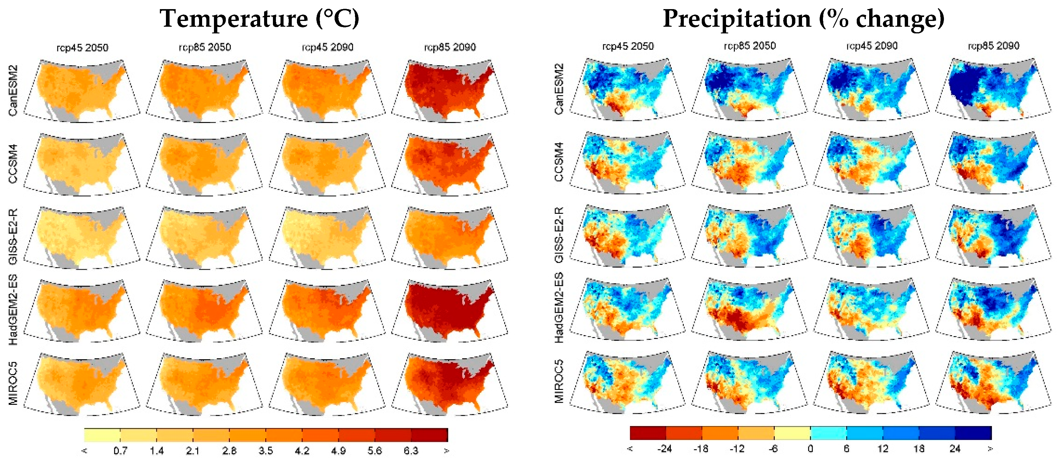RCP4.5 provides a future with additional mitigation on GHG emissions and results in a change in total radiative forcing of 4.5 W/m². Of the many GCMs generated for the AR5, five were selected for this study. These were selected based on multiple objectives, related to the full scope of CIRA2 studies, and capture much of the temperature and precipitation change projected for the CONUS across the broader set of CMIP5 GCMs. The selected GCMs are the CanESM2 (from Canadian Centre for Climate Modeling and Analysis), CCSM4 (Community Climate System Model version 4), GISS-E2-R (from the Goddard Institute for Space Studies), HadGEM2-ES (from Met Office Hadley Centre), and MIROC5 (Model for Interdisciplinary Research on Climate). To select these, the points of mean change in temperature and precipitation across CONUS were plotted using scatter plots (i.e., precipitation change on the X-axis and temperature on the Y-axis). The GCMs selected best represent the variability, or “scatter”, of the full set. More detail is provided in Supplementary Material. These projections were downscaled using a statistical process that uses a multi-scale spatial matching scheme to select analog days from observations across CONUS [15,16]. This dataset, LOCA (Localized Constructed Analogs; [17]), results in a 1/16 degree resolution for daily maximum temperature, daily minimum temperature, and daily precipitation. Additional climate variables—solar radiation, wind speed, humidity, minimum and maximum daily air temperature, air pressure —required were developed using a binning approach, sourcing the historical values from the Princeton Land Surface Hydrology Group [18] (pp. 3088–3111). More detail on the climate scenario selection and processing is provided in the Supplementary Material. These variables were aggregated, for this analysis, to the USGS 8-digit Hydrologic Unit Code (HUC-8) scale (more detail on the HUC can be found in [19]). Furthermore, each climate projection through 2099 is split into two 20-year “eras”: 2050 (2040–2059) and 2090 (2080–2099). These eras are compared to a 20-year baseline climate of 1986–2005. Average changes in temperature and precipitation across the LOCA scenarios and over time are displayed in Figure 1.

Note that in the results section (Section 3), we often focus on two GCMs (rather than the full set of 5 GCMs) for simplicity of presentation—namely, GISS-E2-R and MIROC5. These GCMs represent two extremes as pertains to water quality and exhibit different spatial patterns of changes in climate. The GISS-E2-R climate model projects less increases in air temperature than the others, with wetter conditions in the East. Alternatively, the MIROC5 climate model projects high increases in air temperature and considerable drying, especially in the central region of CONUS. The full set of the results for the five GCMs is provided in the Supplementary Material.

2.2. Description of HAWQS

The Hydrologic and Water Quality System (HAWQS; [11]) is a web-based Decision Support System developed at the Texas A&M University Spatial Sciences Laboratory and funded by the United States Environmental Protection Agency (EPA) Office of Water. HAWQS is an advanced, total water quantity and quality modeling system with databases, interfaces and models that evaluates the impacts of proposed regulations, water quality management actions and scenarios of climate and land use change on the quality and quantity of the Nation’s streams and rivers.

The core engine of HAWQS is the watershed water quality and quantity simulation model, Soil and Water Assessment Tool (SWAT). Originally developed by the U.S. Department of Agriculture (USDA), SWAT has been the core simulation tool for numerous US national and international assessments of soil and water resources. SWAT is a physically-based, computationally efficient model that continuously simulates a large array of watershed processes for a defined period of record. Details of the SWAT modelling methods are described in the Theoretical Documentation [20].

HAWQS is designed to support national-scale economic benefit assessments of potential water quality management strategies (including policy scenarios and best management practices), and is capable of supporting a wide variety of national- and regional-scale economic and policy analyses by simulating baseline and alternative water quality conditions for sediments, pathogens, nutrients, biological oxygen demand, dissolved oxygen, pesticides, and other characteristics. The model follows a broad modeling sequence: (1) the landscape phase, where the primary processes are climate, soil water balance, nutrient and sediment transport and fate, land cover, plant growth, farm management; and (2) the main channel phase, where the main processes are river routing, sediment and nutrient transport through the rivers and reservoirs. While HAWQS is capable of modeling CONUS at the spatial scale of the 10- and 12-digit HUC, the 8-digit HUC is used in this study.

2.2.1. Landscape

In HAWQS, runoff is modeled using the Soil Conservation Service (SCS) curve number procedure on a daily basis, adjusting for antecedent soil moisture, canopy interception (thus effective rainfall), land cover, slope and soil type. The parameters for this calculation are collected from United States Department of Agriculture—Natural Resource Conservation Service, State Soil Geographic [21] and topography from [22]. The simulated buildup and transport of nutrients and Biological Oxygen Demand (BOD) in the landscape are modeled in HAWQS in response to agricultural management, municipal point-sources, and atmospheric deposition [23]. Agricultural land use data were derived from the National Agricultural Statistics Service [24]. In the landscape, solar radiation, relative humidity, minimum and maximum daily temperature, and wind speed, and leaf area, are used to estimate crop growth and runoff.

2.2.2. Main Reach and Reservoirs

The daily estimates of runoff, lateral and ground water flow including any contribution from tiled land surfaces are added to the main routing stream after routing through the tributaries for channel losses. Once the water is added to the main routing, the water is routed using variable storage coefficients [25] (pp. 100–103) through each 8-digit HUC reach with point sources added in each reach based on the contribution of nitrogen and phosphorus by population. If reservoirs are present, the SWAT routes water, nutrients and sediment through the reservoirs based on their characteristics. Reservoir information is sourced from the National Inventory of Dams [26]. River flows, derived from the United States Geological Survey [27], were used for calibration and validation of the flow at selected locations across CONUS. Water consumptive use data were sourced from [28] for surface and groundwater uses.

Within each 8-digit HUC, the main river reach and reservoirs are assumed to be well-mixed. Water temperature is calculated based on dampened changes in daily air temperature developed by [29]. The transport of nutrients, dissolved oxygen, and sediment in streams is modeled in the stream by keeping track of changes in mass on a daily basis. All details of SWAT calculations are well-documented in [20].

2.3. Description of US Basins

The version of the US Basins model used here is described in [8] (pp. 1326–1338). Precipitation and temperature from each climate scenario are inputs into: (a) a rainfall-runoff model (CLIRUN-II), which is used to simulate monthly runoff; and (b) a water demand model, which projects the water requirements of the municipal and industrial (M&I) and agriculture sectors. With these runoff and demand projections, a water resources systems model produces a time series of reservoir storage, release, and allocation to the various demands in the system, which include M&I, agriculture, transboundary flows, and hydropower. The water quality model is driven by QUALIDAD [30], which uses managed flows and reservoir states to simulate a number of water quality constituents in rivers and reservoirs. Since US Basins does not include a representation of loading transport through the landscape, loading into the main river reaches is exogenous. For this study, nonpoint agricultural loadings from the HAWQS landscape (phosphorus, nitrogen and BOD) are used directly in US Basins, equally distributed across each segment within the HUC-8. Due to the computational intensity of US Basins, one year of mean climatology is used for the baseline period and future eras.

2.3.1. Runoff and Water Demand

The climate projections for each emission scenario were used to develop monthly runoff estimates. Runoff modeling converts the climate shifts into changes in surface water availability important for the water resource systems model. Surface water runoff was modeled with the rainfall-runoff model CLIRUN-II (see [31,32]), the latest available application in a family of hydrologic models developed specifically for the analysis of the impact of climate change on runoff, first proposed by [33] (pp. 1–16). Water demands are the other side of the water balance, and are developed using 2005 data from the U.S. Geological Survey on annual water withdrawals and consumptive use in a range of sectors including irrigation, M&I use, mining, thermal cooling, and several other sectors [34] (p. 52). These data are available at the 3109 counties of CONUS and spatially averaged to the 8-digit HUC resolution using the same approach taken by the U.S. Forest Service in their development of the Water Supply Stress Index (WaSSI; [35]).

2.3.2. Water Resources Planning Model

Reservoir management and routing in US Basins is simulated using a water resource systems scheme, where the simulated runoff—used as surface water supply—and projected water demands are used to optimize water allocation based on a prescribed set of priorities. Three demand types, or nodes, are modeled throughout the system, which are in competition for water dependent on the sequence (upstream/downstream). The node types are municipal and industrial (M&I) water use, hydropower generation, and irrigation withdrawal. The hydrologic boundaries used to define the basins are the 2119 8-digit HUCs of CONUS. The structure of each basin is generic, prescribed with input characteristics that are unique to each HUC. Reservoir data, such as locations, hydropower capabilities, and the information needed to calculate surface area and volume are all retrieved from the Army Corps of Engineers [26]. Hydropower production is calculated and calibrated to the National Renewable Energy Laboratory (NREL) Regional Energy Deployment System (ReEDS) model [36] (pp. 275–3000). For each of the basins, the priorities of the various water users are assumed to be in the following order: (1) minimum flows driven by environmental and trans-boundary concerns; (2) M&I water demands (including mining and thermal cooling); (3) irrigation demands; and (4) hydropower production. More detail on the calibration and verification of US Basins can be found in [37].

2.3.3. Water Quality Model Description

Using the managed flows and reservoir storage and volume from the water planning model as well as climate parameters, we use the QUALIDAD model [30] to track several water quality constituents for each 8-digit HUC, including temperature, dissolved oxygen (DO), three nitrogen species, two phosphorus species, a generic metal, and salt. QUALIDAD is a parsimonious water quality model that is designed to model daily water quality dynamics at the basin scale. The mathematical representations of these processes are detailed in [30]. The mass balance equation is solved numerically using the Matlab Ordinary Differential Equation (ODE) 15 s [38] (pp. 1–22). All variables in this model have a daily time step except temperature, which is hourly. For simplicity, monthly flows are transformed to daily using a spline interpolation, which is certainly a limitation the US Basins approach and plans are in place to address this in the future. To track water quality constituents within the CONUS framework, each 8-digit HUC is divided into a number of segments based on the [39], which is a dataset built upon the EPA’s digital record of over 60,000 river reaches in the U.S., intended for national water-quality modeling. For each river segment, the data set contains corresponding parameters such as flow, velocity, segment length, and the sequence of segments. Based on these parameters, the main river channel is found within each 8-digit HUC, and then separated into segments based on travel time estimates optimized to reduce numerical dispersion. Each constituent is modeled separately in each segment, and upstream to downstream mass transfer is governed using numerical methods documented by [30,31]. More detail on the CONUS routing framework is provided in [40].

Temperature is tracked within QUALIDAD using a heat budget model approach [41], that simulates the surface heat exchange of a body of water as well as water sources/sinks through inflows from upstream basins, outflows downstream, small tributaries, and groundwater. Strzepek [40] includes more detail on this approach. We assume that each riverbed is parabolic, following [42], which helps to derive a relationship of flow with surface area and velocity. Wind speed, relative humidity, daily temperature range, solar radiation, and air pressure are used in addition to precipitation and temperature to calculate water temperature.

In the summer, as temperature warms and solar radiation increases, stratification in temperate reservoirs occurs. Temperature during the season of stratification is modeled differently for reservoirs, where a two-layer model is used, representing both the epilimnion (top) and the hypolimnion (bottom) layers. For example, if the reservoir is bottom-releasing (i.e., outflow is occurring in the hypolimnion) then the water state (e.g., dissolved oxygen levels) in the bottom layer flows downstream.

A detailed sensitivity analysis of this process-based mass balance approach that governs the water quality calculations of US Basins can be found in [8] (pp. 1326–1338).

2.4. Summary of Key Differences between US Basins and HAWQS

There are several key differences between the HAWQS framework and the US Basins framework (summarized in

Table 1. Summary of key differences between US Basins and Hydrologic and Water Quality System (HAWQS).

Parameter/Characteristic	US Basins	HAWQS
Number of years per “era”	One year	20-years
Runoff model	CLIRUN, calibrated, monthly	SWAT, daily
Landscape	Simple	Complex, includes land management, fertilizer application, more complex crop model, among others
Water quality model	QUALIDAD, daily	SWAT, daily
Reservoirs	Stratified, 2-layer	Well mixed with seasonal settling and decay rates
Main Rivers	Multiple segments per HUC8	Well mixed
Water Allocation/management	Priority scheme, hydropower, monthly	Based on a calibration of flows, daily
Water Temperature	Energy balance, hourly	Dampened air temperature, daily
DO saturation	Based on temperature and elevation	Based on temperature

). To start, US Basins is computationally intensive, due to the ODE solver, and for this study mean climate conditions are used for each era and scenario, as discussed. Alternatively, HAWQS runs the full set of transient years, resulting in 20 years for each era and scenario. The process of converting climate into flow is estimated differently. Although HAWQS is not fully calibrated across CONUS, HAWQS has been calibrated and verified across large areas of CONUS [43,44]. Then, runoff, routing, and water withdrawal is translated into flows based on a pre-calibrated scheme. On the other hand, US Basins uses estimates of naturalized runoff to calibrate the runoff model on a long-term mean monthly basis across CONUS. These runoff estimates are applied to a prioritization scheme of water uses to estimate flow and reservoir levels. Furthermore, US Basins focuses on the water quality of the main reach, lacking many of the landscape and tributary processes applied in HAWQS, which includes 225,000 landscape units distributed across CONUS. The loadings between the two models are also different, discussed in detail in Section 2.5.

Although the water quality models both use many of the same mass balance equations in-stream as outlined in [41], the application is different. HAWQS solves these mass balances on a daily basis assuming the main reach and reservoirs are well-mixed and the water temperature equation is estimated based on air temperature. US Basins splits the main reach into segments, as described previously, and the reservoirs into two vertical layers to account for summer stratification. In addition, these mass balance equations in the reach and reservoirs are solved numerically using ODE solvers. The water temperature is also solved numerically using an energy balance equation. Additionally, US Basins accounts for the effect of elevation on the DO saturation level while HAWQS DO saturation is based on water temperature only, without the elevation effect.

Many of the specific implications of these differences are discussed in the Results section that follows.

2.5. Loading Inputs to US Basins and HAWQS

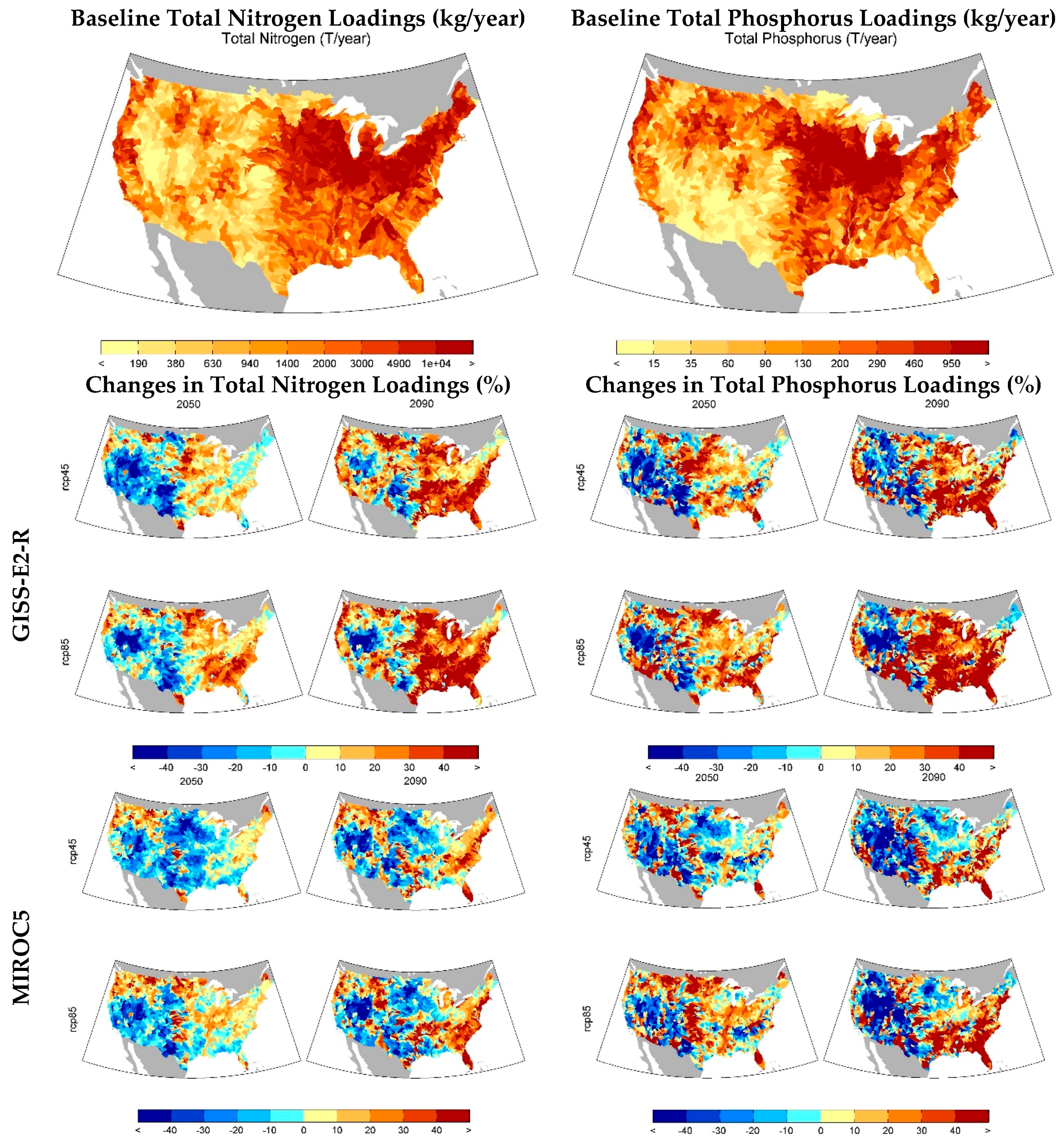
In each model, loadings enter the system as point and nonpoint sources. Agricultural nonpoint source loadings were developed in HAWQS using data available from the Spatially Referenced Regressions on Watershed Attributes (SPARROW) model (see [45]). These included total annual nitrogen and phosphorus from fertilizer application, as well as BOD outputs from livestock. Non-point loadings were modeled using HAWQS to estimate the transport of nonpoint loadings to the main river reaches and reservoirs. These loadings vary with runoff, as SWAT includes crop, tree, and plant nitrogen, phosphorus, and carbon cycles. The longer the nutrients stay in the soil, the more they are consumed by vegetation. As climate change affects runoff, each climate scenario has a unique set of nitrogen and phosphorus loadings from agriculture (see Figure 2). Note the similarities between the inverse of changes in precipitation (Figure 1), and the changes in loadings presented below.

In both HAWQS and US Basins, loadings from municipalities were estimated using export coefficients for both nitrogen (2 kg/person/year) and phosphorus (0.3 kg/person/year) derived from [46]. BOD loadings from municipalities are excluded. These annual per capita loadings were scaled to kilograms based on U.S. population projections developed using the Integrated Climate and Land Use Scenarios (ICLUS, version 2 [46] (pp. 20887–20892); [47]) model. Using the UN Median Variant projection for the U.S. [47], ICLUSv2 was applied to generate county-level population projections at five-year time steps between 2000 and 2100, which were then spatially averaged to the 8-digit HUCs. This population projection is consistent across both GHG mitigation scenarios. These point source loadings rose proportionately to projected population through 2100. In addition, HAWQS includes loadings from atmospheric deposition, which is based on wet and dry deposition from historical observation stations on a monthly basis by 8 digit HUCs [23]. These loadings from atmospheric deposition were excluded in US Basins because US Basins lacks a model of the landscape as discussed previously.

2.6. Valuation of Water Quality

In this study, the economic impacts of changes in water quality measures are estimated using a valuation of changes in a water quality index. Many water quality indices have been developed over the past 50 years. The National Sanitation Foundation (NSF) (explained in detail in [48]) built on previous work by incorporating expert judgement and provides a template for many water quality indices developed since (e.g., [49]). In this study, we use a water quality index following a similar approach outlined by [49], which follows three steps: (1) obtain measurements on water quality constituents, obtained directly from the water quality model previously described; (2) convert each measurement into a subindex using water quality curves and (3) aggregate the subindex values into the WQI. McClelland [48] provides water quality curves (step 2) and aggregation weights (step 3) for nine water quality parameters. Using this approach, we develop a “Climate WQI” (CWQI) similar to the one used in [8] (pp. 1326–1338), which uses four subindex calculations: water temperature, as well as the concentrations of DO, total phosphorus, and total nitrogen. In this study, we use an updated form of the subindex calculations for DO, total nitrogen and total phosphorus from [50]. The subindex curves vary for total nitrogen and total phosphorus across the U.S. by Level III Ecoregion and are based on a fitted exponential function. In contrast, the DO subindex curve, based on an exponential relationship below saturation and a second order polynomial above saturation, is the same across CONUS. The temperature subindex calculation [48] is based on deviations from mean water temperature and described in more detail in [8] (pp. 1326–1338). More detail on the subindex calculations can be found in Supplementary Material.

Similar to [8] (pp. 1326–1338), the relationship between changes in CWQI and changes in WTP—used here as an indicator of economic costs and/or benefits—is developed from the full linear meta-regression transfer function from [7], using a piecewise linear function. We use state-level data from the [50] on persons per household to convert WTP per household to WTP per person to develop a national WTP across scenarios and eras. Van Houtven [7] also distinguished WTP by users and non-users. We use state-level boating survey data [51] to weight each 8-digit HUC by fraction of users and non-users. Although “users” include a broader group than boaters, information on other categories was not available at the national level. Both the users/non-users and persons per household are scaled using the population projections discussed previously. The four water quality parameters in each HUC-8 are aggregated, weighting by total HUC-8area, to the Level-III Ecoregions. Because boaters are a subset of all users, and because users have a higher WTP per person than non-users, our approach likely underestimates aggregate WTP for improvements in the CWQI.

3. Results and Discussion

The following section outlines the water quality parameters from the models, starting with the baseline followed by the future projections. As mentioned, these focus on flow, water temperature, total nitrogen, total phosphorus, dissolved oxygen, and CWQI, followed by WTP. The section continues with a more quantitative comparison of the two water quality models and a short discussion.

3.1. Baseline Model Outputs

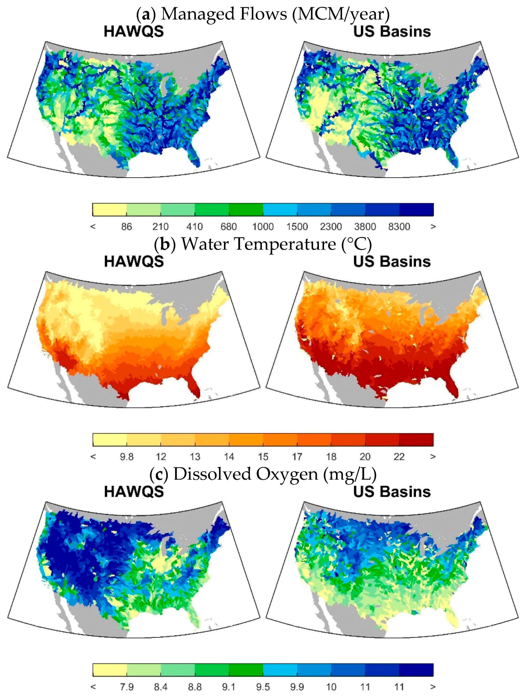
In this section, we describe the main differences in the baseline water quality parameters from both models and identify the main causes for these differences. Figure 3 shows the mean baseline managed flow, water temperature, and DO concentrations. Overall, the spatial patterns of flow between HAWQS and US basins are quite similar, although the magnitudes of flow differ, particularly in the western US where HAWQS flows are higher. These differences are not unexpected, as the US Basins model relies on a calibrated rainfall-runoff model (CLIRUN-II), whereas the HAWQS simulates runoff using partially calibrated curve numbers in SWAT. The lower western river flows in US Basins result in higher nitrogen and phosphorus concentrations in these rivers than in HAWQS. The situation is comparable with DO, where the spatial patterns between the two models are quite similar, although the magnitude of concentrations is generally higher in HAWQS. As discussed previously, SWAT does not adjust for elevation in the DO saturation equation, resulting in higher DO values in high elevation regions in CONUS as compared to US Basins. As for water temperature, US Basins tends to estimate higher water temperatures than HAWQS across CONUS. This is not unexpected since the water temperature in HAWQS (also in SWAT) does not take into account solar radiation, relative humidity, and water depth, while US Basins includes these effects. Also note that US Basins is using a single mean climate year, and does not include inter-annual variability, which also accounts for many of these differences. This also applies to the remainder of the results.

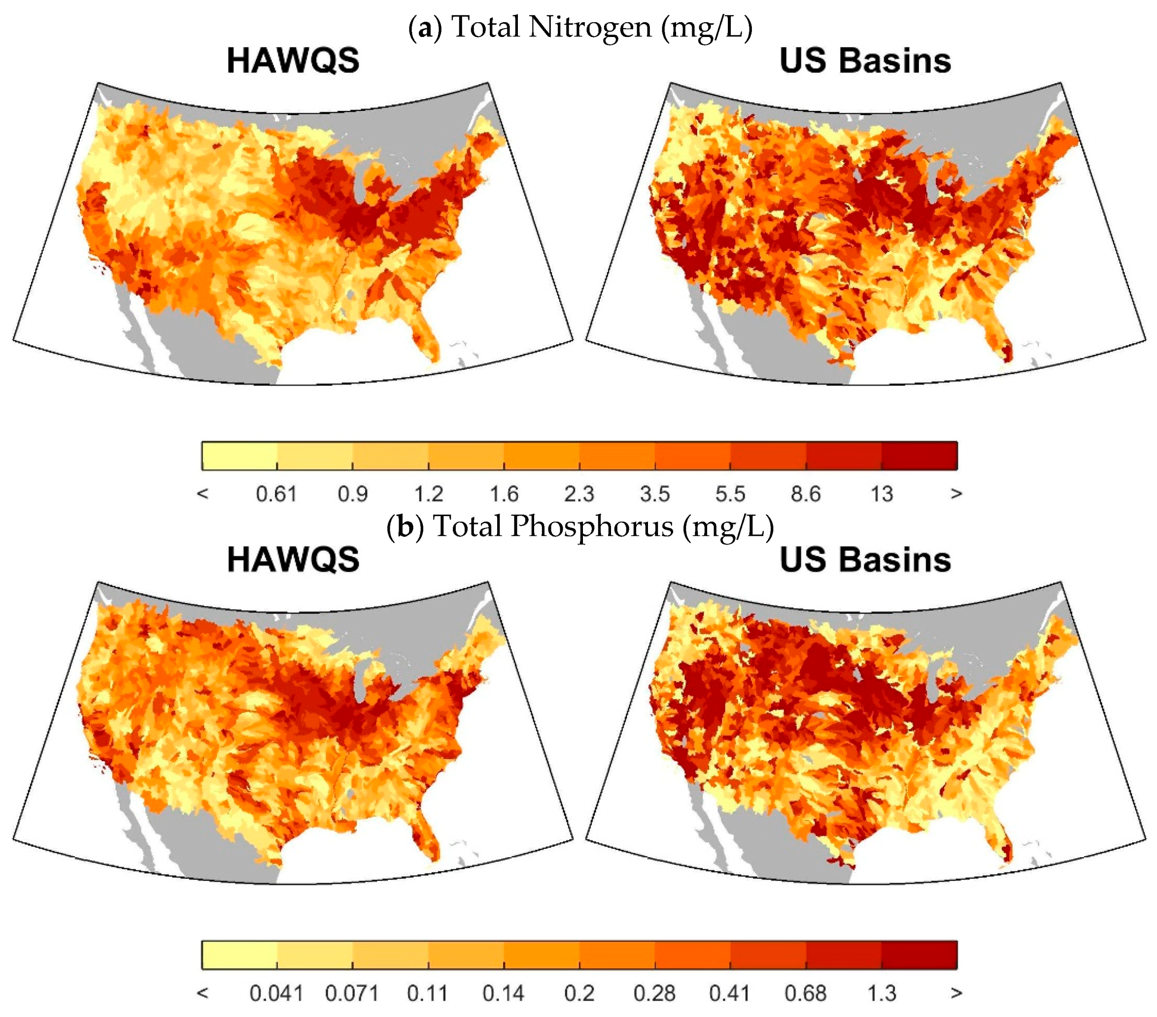
Figure 4 shows the median total phosphorus and total nitrogen concentrations in the main reach in each HUC-8. Both the spatial patterns and magnitudes of each constituent are similar across the two models. As noted above, concentrations in US Basins are higher than HAWQS in the western US because of lower river flows. Also, US Basins uses monthly flows, which cannot account for intra-monthly variations in flow. This also results in differences in concentrations. In addition, US Basins excludes atmospheric deposition while it is included in HAWQS. Atmospheric deposition primarily influences nutrient concentrations in areas with higher precipitation, especially in eastern CONUS.

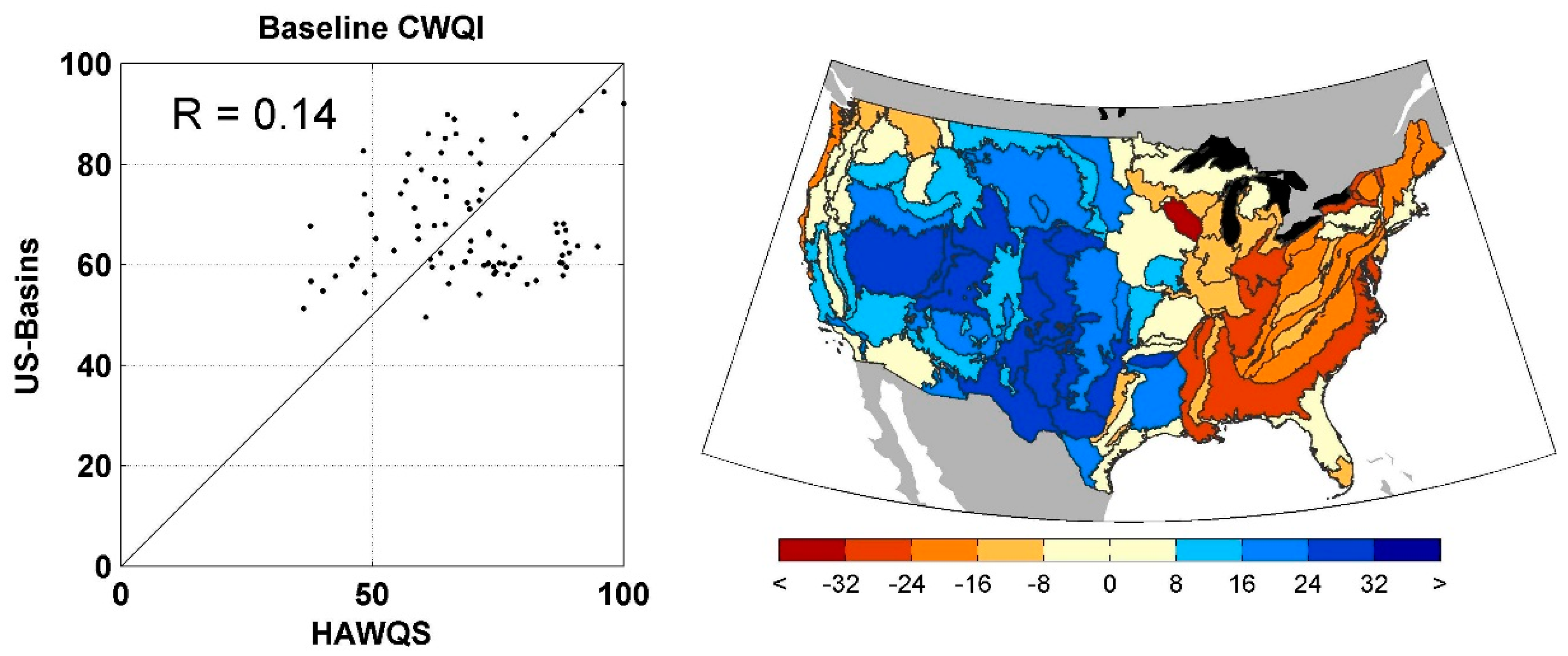
Figure 5 shows the scatter plot of the baseline CWQI across the 85 Level III Ecoregions as well as a map of the differences, where positive values indicate that HAWQS WQI is higher than US Basins. There is a clear difference between the east and west, where HAWQS WQI is higher in the west and US Basins is higher in the east. These differences illustrate two of the major differences in the models. The lower CWQI values in the west in US Basins is primarily driven by lower managed flows in the west than in HAWQS, where lower flows results in higher concentrations of nitrogen and phosphorus and lower DO. In the east, these differences are primarily driven by the additional loadings in HAWQS through atmospheric deposition.

3.2. Projected Model Outputs

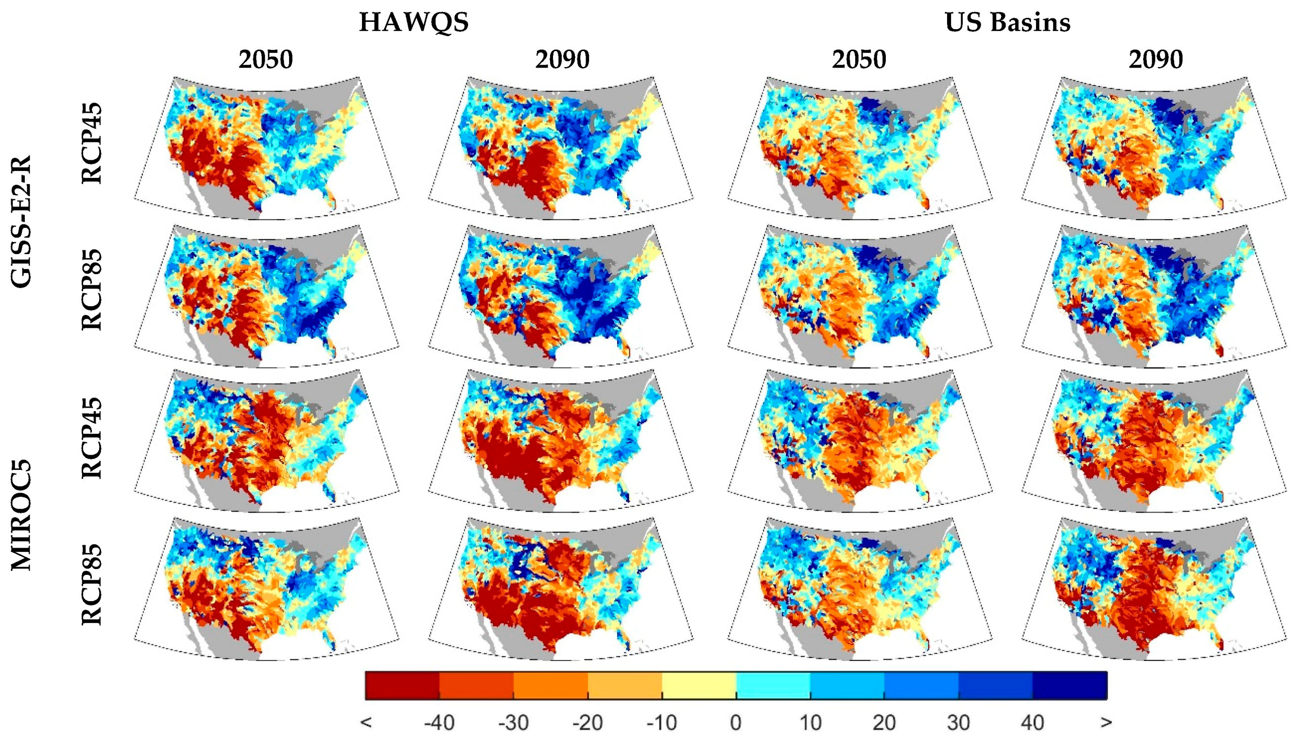
Next we focus on the projections of these water quality parameters under climate change. As noted in Section 2.1, we focus on two GCMs for simplicity—GISS-E2-R and MIROC5. Figure 6 shows the change in managed flows for both water quality models for 2050 and 2090. Both water quality models generally project larger changes in flow in 2090 than 2050. There are also a number of differences between flow projections. For GISS-E2-R, HAWQS projects larger decreases in the flow in the southwest than US Basins, while US Basins projects larger decreases in flow in the central portion of the country. The increase in flow in the east is consistent across both HAWQS and US Basins. For MIROC5, both HAWQS and US Basins project decreases in flow in the central portion of CONUS with less change in the east and slight wetting in the northwest. The most striking difference between HAWQS and US Basins in MIROC5 is the southwest, where HAWQS projects large decreases. However, this portion of the country is dry, so the relative change (as shown in percent) is large but the total change in flow smaller than other portions of the country. These differences between the water quality model projections of managed flow represent a complex interaction between changes in climate, modeled runoff, and the model assumptions about reservoir management.

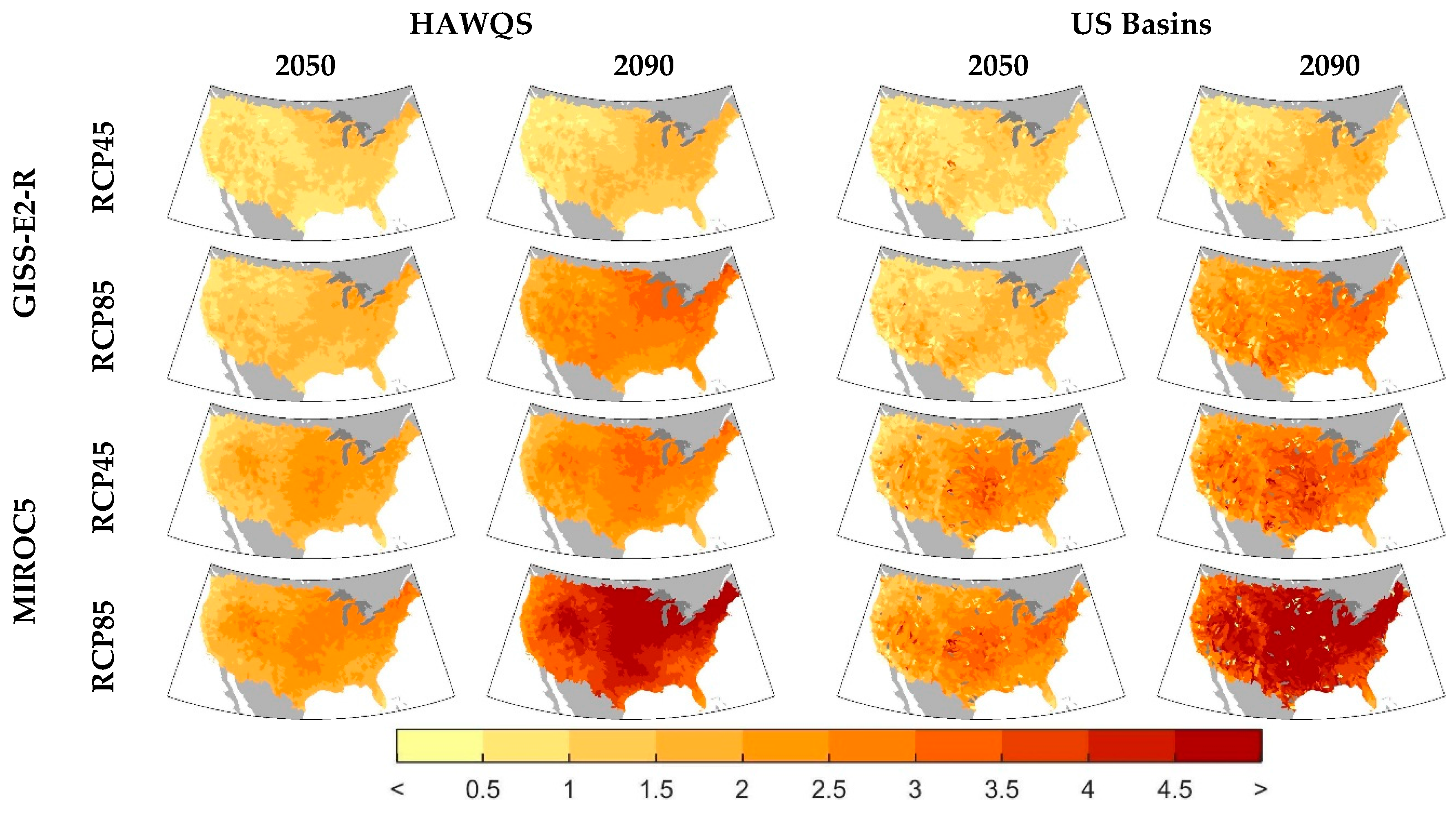
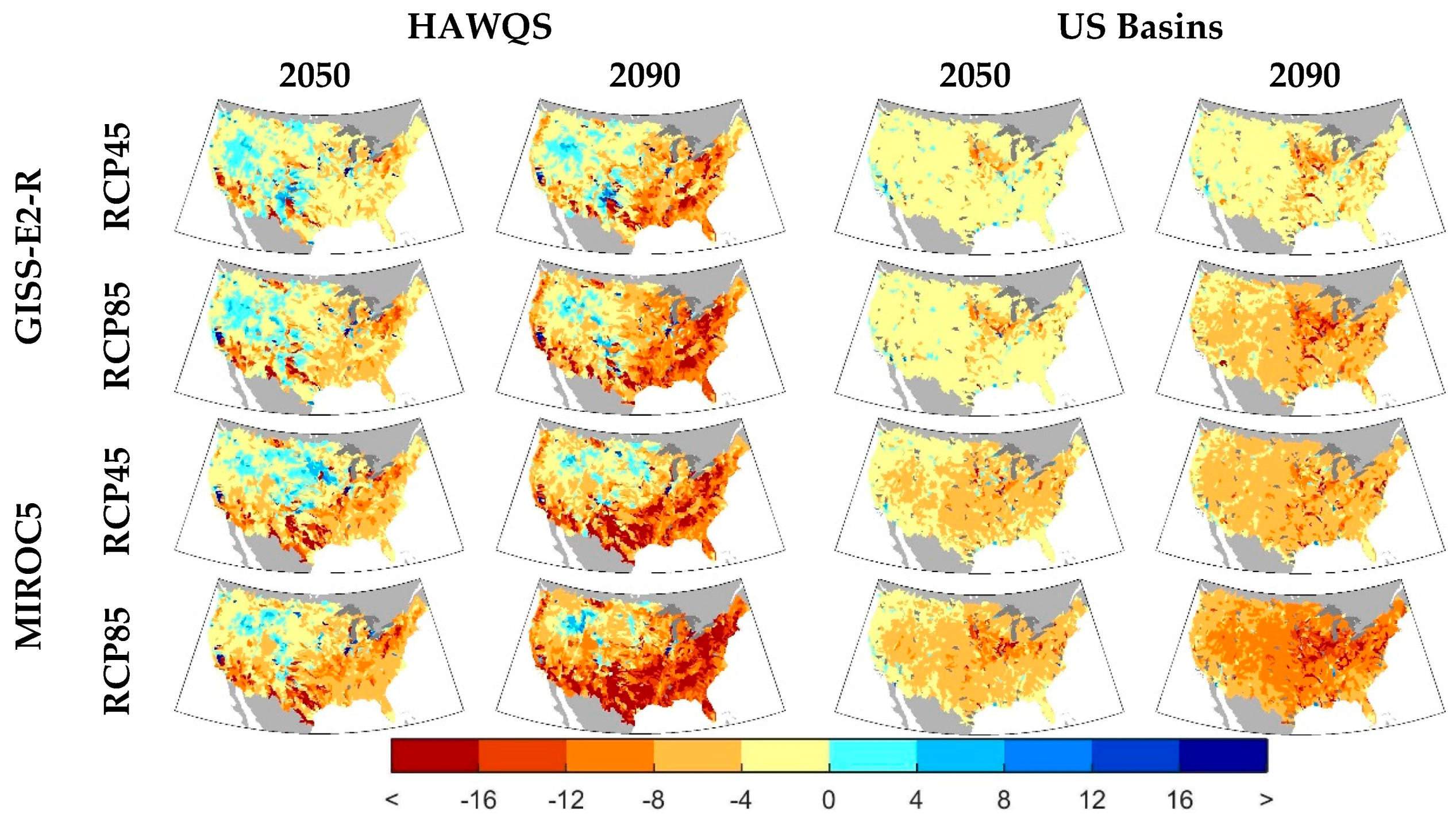
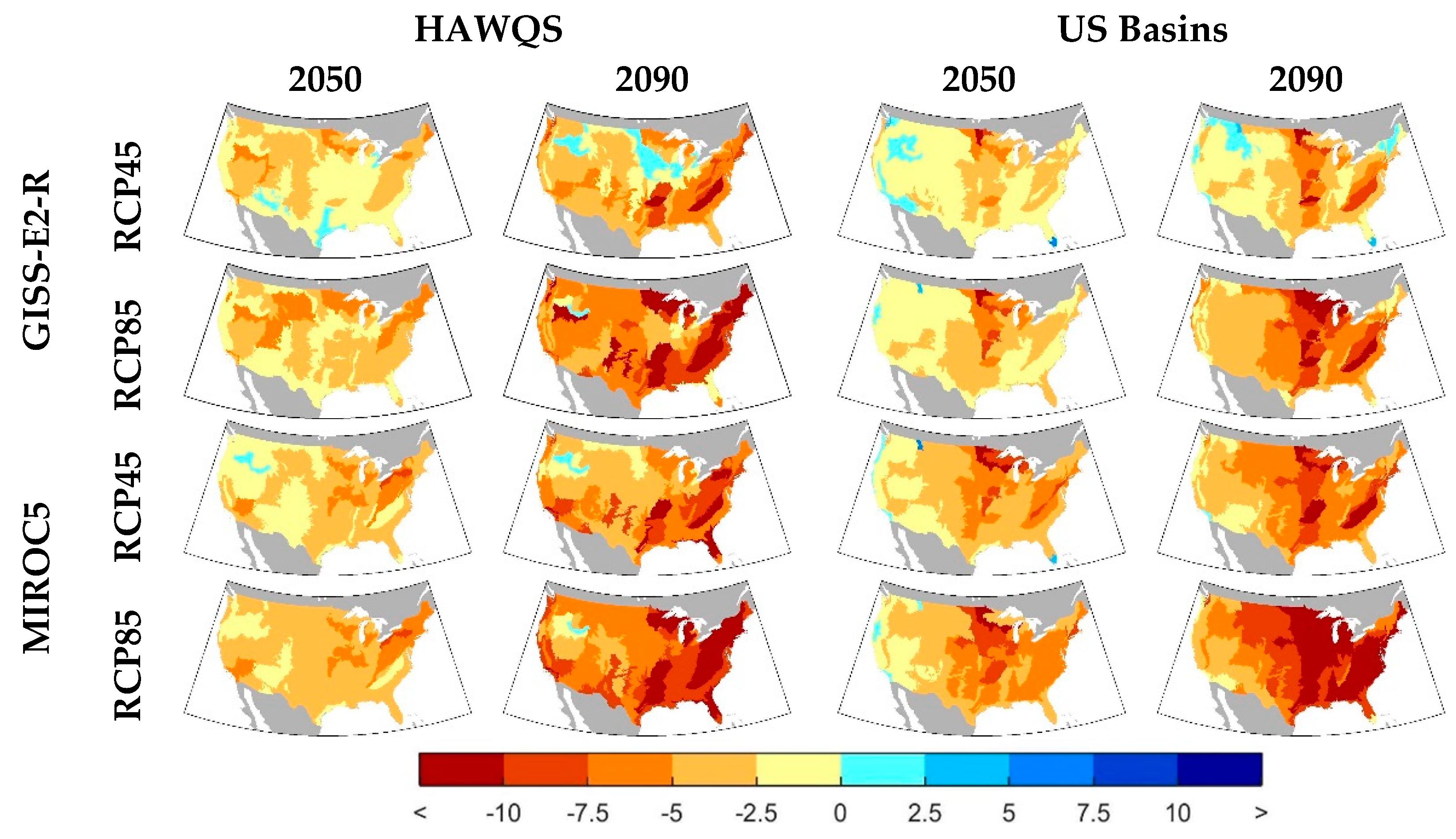
Figure 7 shows the changes in water temperature for both climate models and water quality models in 2050 and 2090 and both RCPs. Since water temperature is primarily driven by changes in air temperature, this water quality parameter shows the most similarity between the two water quality models. However, the two models estimate water temperature using completely different equations, as previously discussed. These, along with the differences in changes in runoff and flow account for the different spatial patterns shown for the two models. The 2050 results show moderate increase in water temperature, while the results in 2090 are more extreme with increases above 4.5 °C in MIROC5, RCP85.

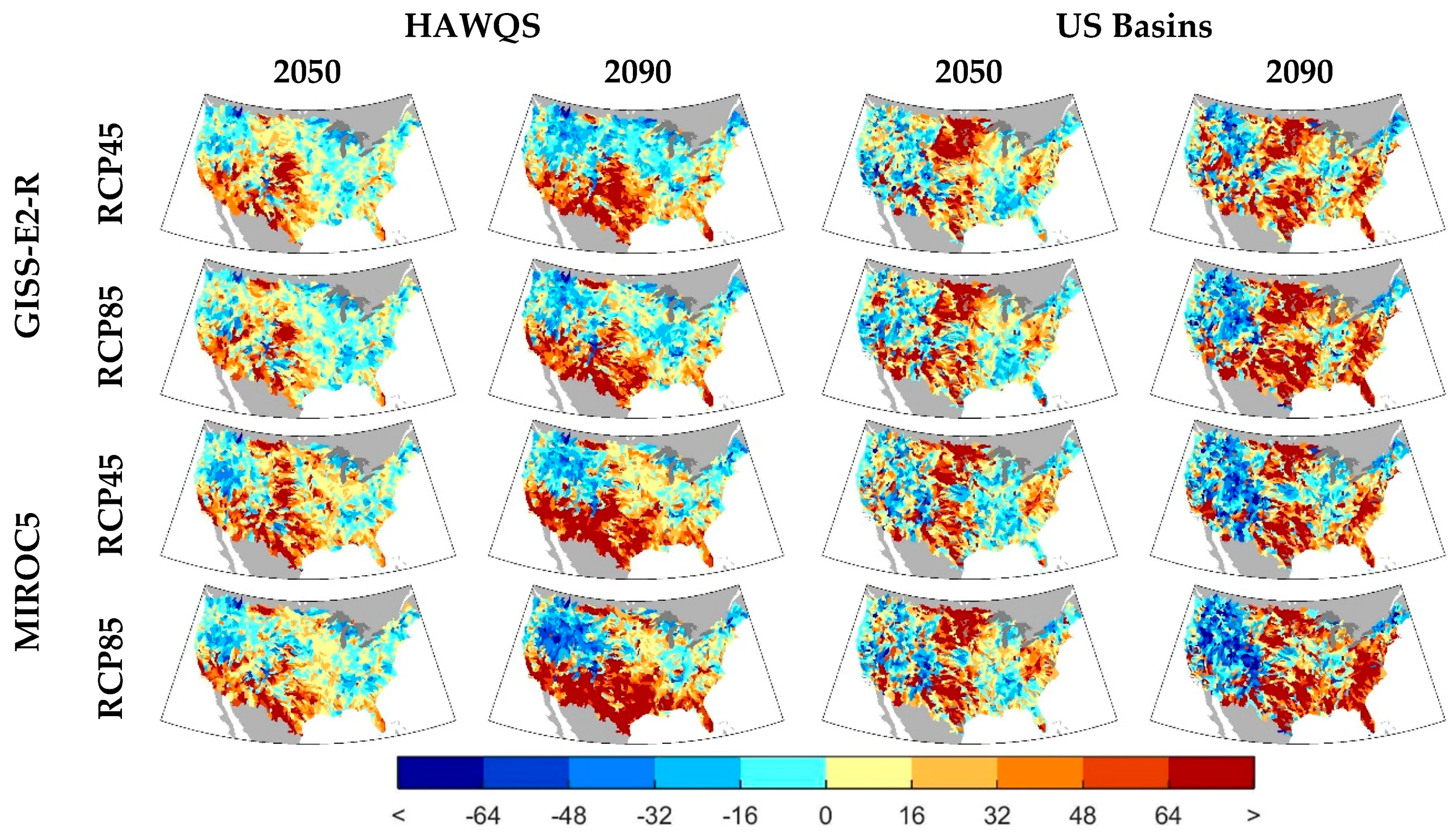
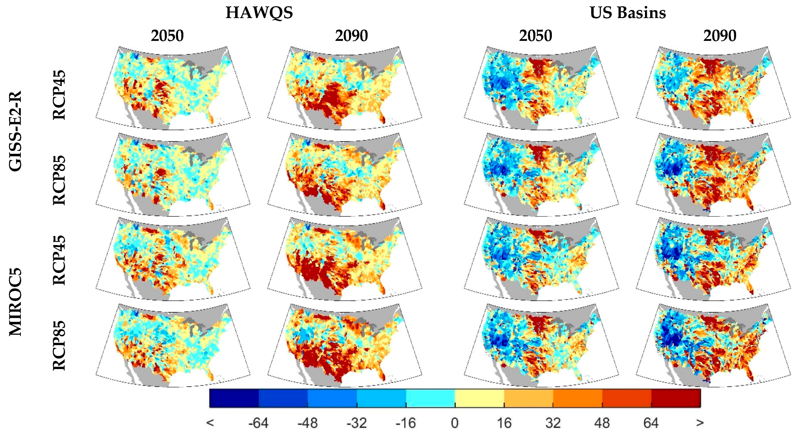
Figure 8 shows the percent change in total nitrogen concentrations. Both models show larger changes in 2090 than in 2050. Both water quality models agree that the south-central U.S. and the area around the Great Lakes are likely to see increases in total nitrogen. HAWQS shows large increases in total nitrogen in the southwest for all GMS and RCPs in 2090, albeit more pronounced in MIROC5 than GISS-E2-R, while US Basins show decreases in this region. Figure 9 shows changes in total phosphorus concentrations across CONUS. HAWQS consistently projects increase in phosphorus levels along the southwest coast and Texas. In contrast, US Basins projects larger increases in the central U.S., especially in 2090, as well as in the east. Differences in nitrogen and phosphorus concentration changes can be explained primarily by the differences in flow changes for these two models. Also notice the differences in the change in concentrations in the drier areas—namely, the southwest—where the models differ in sign. Since flows are low in these areas, the resulting concentrations are sensitive to flow changes.

Figure 10 shows percent changes in DO for the same eras and scenarios. In both water quality models, there are consistent decreases in DO in the east. HAWQS shows large decreases around Texas, areas in the southwest, and along the East coast, with areas of increases in the western mountainous regions. US Basins shows the largest decrease in DO around the Great Lakes. Since DO is largely influenced by temperature through levels of DO saturation (i.e., higher temperatures reduce DO saturation levels, thereby reducing DO aeration), DO generally decreases in the future. However, DO is also influenced by changes in nitrogen, phosphorus, and BOD loadings, as well as changes in flow. In both models, changes in DO are largest for 2090 as compared to 2050 and larger for RCP85 than RCP45.

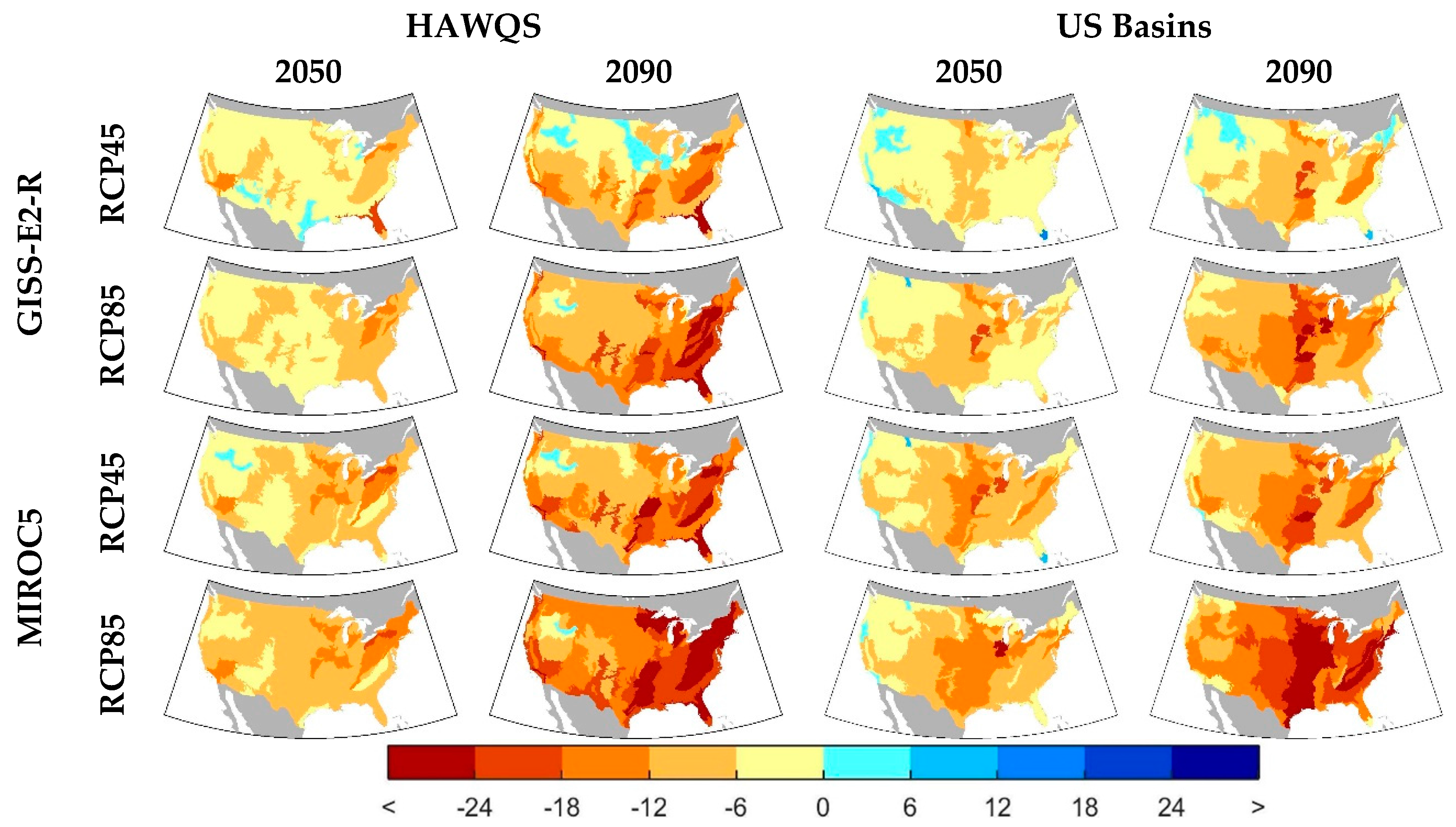
Changes in CWQI are shown in Figure 11. For both water quality models, changes in CWQI are more pronounced in the east than in the west from increases in loadings, causing higher concentrations of total nitrogen and total phosphorus, and temperature being higher in this area. For HAWQS, changes in CWQI are largest along the east coast, although this pattern also shows in US Basins in MIROC5 RCP85. US Basins tends to show larger increases in CWQI in the central U.S. and around the Great Lakes. Since this is an aggregation of the changes in water quality parameters previously discussed, many of these differences between projected CWQI changes can be explained by the model differences already discussed. For example, HAWQS shows larger decreases in CWQI in the west relative to US Basins, for GISS-E2-R in particular. These can be explained by increases in nitrogen and phosphorus in the west as compared to US Basins projections of nitrogen and phosphorus.

Table 2. Correlation coefficients of changes in CWQI across the Ecoregions between HAWQS and US Basins.

		CanESM2	CCSM4	GISS-E2-R	HadGEM2-ES	MIROC5
RCP45	2050	0.08	0.02	0.05	0.31	0.47
	2090	0.21	0.39	0.45	0.33	0.43
RCP85	2050	0.05	0.01	0.21	0.29	0.35
	2090	0.36	0.36	0.44	0.37	0.46

and

Table 3. Correlation coefficients of changes in WTP across the Ecoregions between HAWQS and US Basins.

		CanESM2	CCSM4	GISS-E2-R	HadGEM2-ES	MIROC5
RCP45	2050	0.32	0.14	0.27	0.50	0.59
	2090	0.34	0.38	0.40	0.44	0.42
RCP85	2050	0.33	0.21	0.35	0.51	0.53
	2090	0.50	0.40	0.48	0.48	0.54

show correlations of changes in CWQI and WTP across the Level III Ecoregions for the five GCMs, two emissions scenarios, and two future eras. The least agreement between the water quality models is found in the GISS-E2-R GCM in 2050 for RCP45, which represents the climate with the least change, of the ones shown, in both temperature and precipitation. However, there is more agreement between the water quality models for future climates with higher radiative forcing, either by mitigation policy or era, and larger projected changes in climate as seen in MIROC5.

We find that while the models present a different picture of baseline water quality, the projections of aggregate water quality as expressed through CWQI tend to exhibit stronger levels of agreement and that as changes in climate become more drastic—i.e., in projections of climate with higher solar forcings either in time or global GHG mitigation policy—agreement, across the two models is highest. As discussed, differences in these water quality projections from the two models point to dissimilarities in the model structure and inherent bias of each water quantity and quality model. As these are complex systems modeled over large geographic areas, inconsistencies in the outcomes of the two models are expected. However, we find greater levels of agreement across the water quality models in the direction and magnitude of CONUS-wide climate change impacts.

3.3. Valuation

The following section focuses on the valuation results, in terms of changes in WTP, for both water quality models at the Level III ecoregions. Figure 12 shows these WTP changes, in 2005 USD/year/person for the two climate models, two eras, and two mitigation policies. Note that decreases in WTP reflect the willingness to pay in order to avoid the given water quality scenario relative to the baseline. Since these values are directly related to the changes in WQI, these maps resemble the maps in Figure 11. Although there are differences in WTP changes across the two models, both models consistently show decreases in WTP in the future, with few increases across ecoregions. Decreases under RCP45 are smaller, generally, than under RCP85, with this pattern more pronounced in 2090 than 2050. WTP decreases are more pronounced particularly in the east on all counts than in the west. HAWQS continues to show more impacts on the west coast than US Basins, while US Basins shows more consistent increases in WTP in the Midwest, and the lower Mississippi basin.

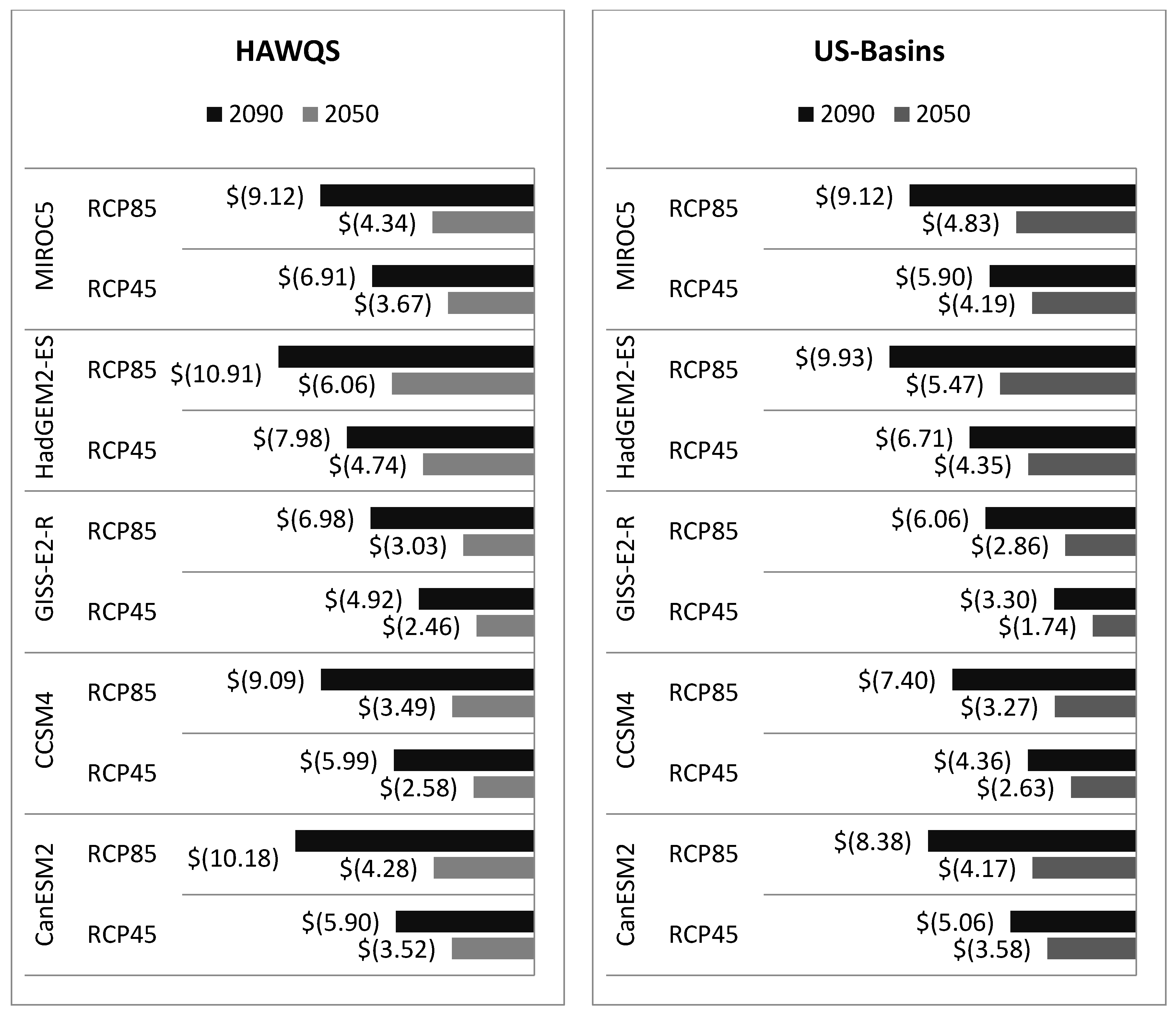
National level WTP per person is shown in Figure 13 and total WTP is shown in in

Table 4. Total WTP (in billion 2005 USD/year) for all five GCMs and global GHG mitigation scenarios.

			CanESM2	CCSM4	GISS-E2-R	HadGEM2-ES	MIROC5
RCP45	2050	HAWQS	−$1.36	−$1.00	−$0.95	−$1.83	−$1.42
		US-Basins	−$1.38	−$1.01	−$0.67	−$1.68	−$1.62
	2090	HAWQS	−$2.59	−$2.62	−$2.16	−$3.50	−$3.03
		US-Basins	−$2.22	−$1.91	−$1.45	−$2.94	−$2.59
RCP85	2050	HAWQS	−$1.66	−$1.35	−$1.17	−$2.34	−$1.68
		US-Basins	−$1.61	−$1.26	−$1.10	−$2.11	−$1.87
	2090	HAWQS	−$4.46	−$3.98	−$3.06	−$4.78	−$4.00
		US-Basins	−$3.67	−$3.24	−$2.66	−$4.35	−$4.00

for all five GCMs, RCPs, eras, and the two water quality models. In all GCMs and water quality models, WTP decreases most for RCP85 compared to RCP45. The largest changes in WTP are shown in the HadGEM2-ES GCM with the least projected for GISS-E2-R. Differences between these two GCM projections for both water quality models are 3.9 USD/person/year for RCP85 in 2090. In contrast, the largest difference between the two water quality models for RCP85 in 2090 is 1.8 USD/person/year for CanESM2. Since CanESM2 shows the largest changes in precipitation, this difference in WTP between the water quality models can be explained in part by the absence of atmospheric deposition in US Basins.

4. Conclusions

We find that, as the end-goal of this study is about national scale economic benefits, differences between the increases in WTP for the two water quality models is less than differences between the five GCMs. Decreases in total national WTP in RCP85 range from 1.2 to 2.3 (2005 billion USD/year) in 2050 and 2.7 to 4.8 in 2090 across all climate and water quality models. Converted to a net present value, discounting at 3% and using the mean WTP across GCMs, results in a total decline in WTP of $28.9 and $26.3 billion for RCP45 for HAWQS and US Basins, respectively. For RCP85 this value is $38.2 and $35.8 billion for HAWQS and US Basins, respectively. The overall benefit of GHG mitigation is substantial, at a present value of $9.3 (HAWQS) and $9.5 (US Basins) billion for RCP4.5 compared to RCP8.5. These results are similar to the total impacts found in [8] (pp. 1326–1338) using only one GCM, where the net present value of GHG mitigation benefit, using a policy similar to RCP4.5, was found to be $10.7 billion. Note that these WTP estimates are based on recreational value, which is only a portion of the economy likely to be affected by decreases in water quality.

As both HAWQS and US Basins represent complex hydrologic, biochemical, and heavily managed systems over a broad spatial area, there are certainly limitations to the models and data. In general, both models take a parsimonious approach to modeling the system, so instead of rigorous calibration and validation that is typically performed on detailed models of “project-scale” studies, these models use a process-based, mass balance approach in order to assess general behavior and response to a changing climate. The hydrology in both models is at least partially calibrated, as previously discussed. The water quality modelling, on the other hand, is generally uncalibrated and relies on mass balance and commonly used parameters. For this reason, we do not present results at detailed scales in either time or space and rely on large-scale changes from the baseline water quality projection for the purpose of informing policy rather than individual project construction or design. This study is not the first to use either model in this way. SWAT, the basis of HAWQS, has often been used in ungauged basins (e.g., [52,53,54]) and US Basins was also designed for this type of analysis. However, this is a limitation, and detailed analysis should be performed on a case-by-case basis when needed. Another limitation is that the WTP values used in this study are based on recent estimates and would likely change in the future. Also, the population projections used in this analysis do not vary by RCP, although the populations are likely to change under different forcing levels. However, this decision was made intentionally, in order to isolate the effects of climate change from changes related to population change. In addition, US Basins is the use of only one “median” year to represent the baseline and future eras.

In this study, we have compared only two water quality models. This work can be expanded by comparing more water quality models to understand how other developed methods for projecting future water quality can result in alternative conclusions. Also, as in all climate change impact studies, we are limited by the spatial scale and uncertainty of the GCMs. Climate-related uncertainties were also not fully addressed here, in part by using a subset of the CMIP-5 models, but also by not including uncertainties related to initial conditions (addressing the chaos in the system), as in [37]. In addition, over the last several decades, large improvements have been made in agricultural and urban water conservation, agricultural soil conservation, farming technologies, urban stormwater and wastewater treatment, and protection of critical natural areas. In recent years, large amounts of agricultural land have been removed from soil conservation programs in order to produce more corn for ethanol, and growth of urban areas has removed large amounts of agricultural land from production. Future modeling efforts can address many of the impacts of land use changes, new agricultural and urban water management technologies, and environmental policies. These and other research endeavors are an important part of understanding the future of water quality in the U.S. and the effect of Climate Change.