Quantifying River Channel Stability at the Basin Scale

1
Department of Geography, University of Portsmouth, Portsmouth PO1 3HE, UK
2
School of Geography, University of Nottingham, Nottingham NG7 2RD, UK
*
Author to whom correspondence should be addressed.
Water 2017, 9(2), 133; https://doi.org/10.3390/w9020133
Submission received: 1 January 2017
/
Accepted: 15 February 2017
/
Published: 17 February 2017
(This article belongs to the Special Issue Stream Channel Stability, Assessment, Modeling, and Mitigation)
Abstract
:This paper examines the feasibility of a basin-scale scheme for characterising and quantifying river reaches in terms of their geomorphological stability status and potential for morphological adjustment based on auditing stream energy. A River Energy Audit Scheme (REAS) is explored, which involves integrating stream power with flow duration to investigate the downstream distribution of Annual Geomorphic Energy (AGE). This measure represents the average annual energy available with which to perform geomorphological work in reshaping the channel boundary. Changes in AGE between successive reaches might indicate whether adjustments are likely to be led by erosion or deposition at the channel perimeter. A case study of the River Kent in Cumbria, UK, demonstrates that basin-wide application is achievable without excessive field work and data processing. However, in addressing the basin scale, the research found that this is inevitably at the cost of a number of assumptions and limitations, which are discussed herein. Technological advances in remotely sensed data capture, developments in image processing and emerging GIS tools provide the near-term prospect of fully quantifying river channel stability at the basin scale, although as yet not fully realized. Potential applications of this type of approach include system-wide assessment of river channel stability and sensitivity to land-use or climate change, and informing strategic planning for river channel and flood risk management.
1. Introduction
Morphological adjustment in alluvial river channels can have significant impacts on flood risk infrastructure, development and habitats and presents numerous challenges for sustainable engineering, river basin planning, channel management and river restoration [1]. The propensity for channel change is related to the availability of stream energy to erode, transport and deposit sediment on the channel perimeter, with adjustments in channel morphology more likely to occur where there are disparities in available energy between successive reaches and variations in sediment supply [2]. Assessment of river channel (in)stability is, therefore, vital to inform appropriate river engineering solutions to local problems and in the identification of unstable reaches adjusting to system-wide instability (disequilibrium), where resources can be targeted and management/restoration efforts prioritised [3,4].
In characterizing broad-scale instability, Lane’s [5] relationship is still widely applied. This states that:
where Q = water discharge, S = channel slope, Qs = bed material load, and d50 = median size of the bed material.
This expression suggests a balance between stream power (the product of Q and S) and the product of sediment load and calibre. A change in any of the variables implies a shift away from dynamic equilibrium towards either aggradation or degradation [6], with equilibrium restored by compensatory adjustments in one or more of the other three variables. In the case of a change in the river’s capacity to transport sediment, Lane’s relationship can be rewritten in terms of total stream power, Ω (= γQS in units of watts per unit stream length, where γ is unit weight of water):
Here, a change in sediment load, relative to changes in bed material size, suggests the river will compensate by adjusting its energy expenditure (sediment transporting capacity) during a period of instability until the relationship balances once more. The mechanisms by which discontinuity in sediment transfer can impact upon channel morphology and, therefore, flood defence and highways infrastructure are complex, although some general relationships can be presented for alluvial rivers. For example, if the volume of sediment supplied to a reach over a given time period is less than the capacity of the reach to transport the volume of sediment through, then erosion of the channel boundary is a probable outcome, which could lead to persistent channel instability through bed scour and/or channel widening (dependent on the relative differences in erodibility between bed and bank materials) and the risk of damaging or undermining flood defence assets or other structures. Lateral instability can also be a secondary response if bed lowering increases bank height sufficiently to initiate mass instability [7]. Conversely, if sediment supply is greater than the transporting capacity, then sedimentation processes are more likely to predominate with potential for channel instability through aggradation and/or channel narrowing. Deposited sediment can be a critical factor in flooding [8,9,10], reducing in-channel conveyance and the standard of protection afforded by defences, resulting in maintenance problems [11,12]. Additional complex responses to channel instability include tributary rejuvenation through headcutting, accelerated rates of lateral mobility in meandering rivers [13,14] and channel widening as flow is deflected around maturing sediment bars, both of which could threaten linear flood defences not set back from the channel.
While Lane’s relationship provides a useful concept to describe the capability of an alluvial stream to adjust its morphology through sediment erosion, transport and deposition processes [15] and has provided a platform to develop more rigorous models of qualifying (e.g., [16]) and quantifying (e.g., [6]) river channel change and framing river restoration methods (e.g., [17,18]), critically it does not state explicitly how channel geometry and/or planform might change, or whether the bed and/or banks are likely to adjust in response to a given sediment imbalance scenario. Also, in some cases, the channel boundary might not be free to adjust or might be responding to other influences not accounted for in the relationship [19] and therefore, despite efforts to extend the relationship to include morphological variables [20,21,22], Lane’s approach remains a qualitative, ‘indicative’ treatment of potential channel instability (degradation vs aggradation) that is not necessarily a reliable predictor of the ‘type’ of morphological response, e.g., bed scour, bank erosion, bar formation or some combination thereof.
Although understanding the significance of (dis)connectivity in sediment transfer through the fluvial system is an enduring focus of geomorphological research (e.g., [14,23,24,25,26,27,28,29,30,31]), the throughput of sediment remains poorly accounted for in the assessment and management of flood risk [4] and integration into river management practices remains challenging [32]. One reason for this is the limited availability of practical tools that flood risk managers can apply routinely at the basin scale. The current impetus towards Natural Flood Management [33] that ‘works with natural processes’ means that interrelationships between fluvial hydraulics, sediment dynamics, habitats and flood risk can no longer be ignored in river basin planning and management [34], thus demanding practical, system-wide approaches to investigate, map, characterise and prioritise river reaches in terms of channel morphology, sediment transfer and channel instability.
A decade ago, the UK Flood Risk Management Research Consortium (FRMRC) anticipated this need, delivering a toolbox of methods and models for ‘accounting for sediment’ in rivers (for overviews see [4,35]), enabling practitioners to investigate flood risk impacts of morphological instability. In the UK, the most widely applied approach for assessing sediment-related problems in rivers within their wider, drainage basin context is the Fluvial Audit [12,36,37,38]. In this approach, a rigorous stream reconnaissance survey is undertaken and complemented by a desk study to characterise the drainage basin (or sub-basin) into discrete geomorphological reaches, designated as predominantly sediment ‘source’ (erosional), sediment ‘transfer’ (in transporting equilibrium) or sediment ‘sink’ (depositional) and prioritise reaches for delivering sustainable river management and restoration. In addressing and delineating system-scale instability, the focus of a Fluvial Audit is not on reach-scale (or sub reach-scale) influences and impacts, with other measures better-placed to investigate local sediment problems and issues (e.g., for instability at bridges see [39,40]).
However, while the Fluvial Audit has proven useful in supporting some types of river project (e.g., river restoration), it provides no quantitative measure of the relative scale of channel instability between reaches and thus an objective, hierarchical framework for strategically tackling instability problems remains beyond the capability of the Fluvial Audit method. This is also the case for other broad-scale assessment methods, for example channel evolution models [41], the River Styles Framework [42] and many of the ‘hydromorphology’ tools currently in use (for a review see [43]).
At the other end of the scale of approaches available to explore sediment transfer and channel stability status within river catchments are one-dimensional (1D) and two-dimensional (2D) numerical models such as HEC-RAS (developed by the U.S. Army Corps of Engineers, USACE, Hydrologic Engineering Centre, HEC), iSIS Sediments (developed through a joint venture between Wallingford Software Ltd. and Halcrow Group Ltd., UK, and now part of the Flood Modeller Suite developed by CH2M) and Mike 21C (developed by DHI Group, Hørsholm, Denmark), all of which estimate rates of sediment transport and simulate bed level change through time, based on river hydrodynamics and the properties of bed sediments. Despite the utility of these morphodynamic models for investigating local channel instability problems and informing site-specific management options, the resources required to run them at the basin scale are often prohibitive in terms of time, data, personnel costs, demanding computational requirements as well as the specialised expertise necessary to develop and calibrate these models. Given these restrictions, detailed sediment and morphological modelling approaches remain highly challenging in their up-scaling to the basin level and capability to achieve acceptable levels of accuracy while meeting the requirement of practical and routine deployment.
The sediment transport equations employed in these models are still, unfortunately, subject to high levels of uncertainty and characteristically only predict transport rates to within, at best, half to double measured values (e.g., [44,45,46,47]), with marked variation in performance and no universally accepted rules available for selecting an appropriate equation. Nevertheless, with a range of river sediment transport models available [48] and a burgeoning suite of coupled catchment erosion-sediment transport models now featuring in the literature [30,49,50,51], together with rapidly-emerging technological advances in remotely sensed data capture and image processing that greatly facilitate model set-up, the near-term prospect of modelling sediment transport at the basin scale with acceptable levels of pragmatism, resourcing, accuracy and uncertainty is considerable but as yet not fully realised.
A practical tool for application in watershed studies must be operational with readily available (and normally limited) data and light project resources, whilst maintaining quantitative accuracy. Conceivably, addressing these constraints requires bridging the gap between qualitative, reconnaissance-based fluvial auditing and quantitative sediment transport modelling. The Sediment Impact Analysis Methods (SIAM) tool is one approach that uses sediment transport calculations and principles of sediment continuity, available within the Hydraulic Design module of HEC-RAS [4,35,52,53,54]. In SIAM, the annualised capacity of a subject reach to transport bed material load is compared with the annualised bed material load delivered from upstream (including inputs of sediment from bank erosion, gullies, etc.) to define reach-scale imbalances in sediment load by size class. In addition, SIAM passes washload through the sequence of sediment reaches until its eventual deposition and contribution to the bed material load. However, despite bed material not actually being routed between reaches, the method is based on sediment transport equations and results will inevitably reflect their considerable uncertainty in estimates. This issue of potential quantitative inaccuracy remains even if a sediment transport function is employed in SIAM that is based on stream power concepts, irrespective of the additional challenges in accounting for all non-channel sediment sources in the budgeting process.
This paper reports the development of a basin-scale, energy-based approach that emerged during the FRMRC research programme in response to recognition of the limitations to practical and routine application of currently available tools for holistic appraisal of channel instability through an entire river system. The objectives of the paper are to (i) investigate the feasibility and practicability of using stream energy imbalance, relaxed from the challenges/limitations of calculating sediment transport rates and loads, as a realistic proxy for characterising river channel instability, and therefore the potential for morphological adjustment, and identifying locations where detailed assessment might best be targeted; (ii) explore the challenges and assumptions associated with data requirements and processing that emerged quickly through application to a case study as potential limitations to both the scientific validity of such an approach and its uptake by practitioners. The approach is considered alongside other emerging methods that have been reported and recent technological advances in large-scale data acquisition that might hold considerable promise in providing the inputs necessary for routine basin-scale modelling and realisation of a quantitative Fluvial Audit as a near-term outcome.
2. Concepts, Methods and Data Acquisition
2.1. Stream Energy Approaches in Fluvial Studies: Underpinning Concepts and Current State of Knowledge
The potential for an alluvial river to reshape its channel perimeter and planform can be expressed in terms of the energy available (after overcoming boundary and internal resistance forces) to perform geomorphological work through eroding, transporting and depositing sediment. The balance between magnitude and frequency of sediment transporting flows as conceived by Wolman and Miller [55] is considered in the determination of the formative flow, the ‘effective discharge’ [56] that transports a greater sediment load than any other discrete flow over a period of years. According to Wolman and Miller [55], while flood flows have the potential to mobilise significant quantities of bed and bank sediments, exchange fine sediments between channel and floodplain and redistribute material that is temporarily stored in a river, they occur too infrequently to be effective over a period of years. In contrast, flows that occur very frequently have insufficient energy to erode and entrain sediment in large quantities.
This is perhaps now regarded as a more general model with an emerging body of evidence suggesting that variability in the flow regime, drainage basin size, bed material type and other factors might be responsible for the observed variation in the frequencies of geomorphologically effective flows (for a detailed review, see [57]). It is recognised that in some cases low flows can make a significant contribution to the total annual sediment load, as discussed by Soar and Thorne [17,57] and corroborated by Sholtes et al. [58], and with climate and land-use change the higher magnitude events in humid, temperate environments might become more significant, geomorphologically, in the future.
A river’s total sediment load is calculated by integrating flow duration with sediment transport rate and is often expressed as the average annual sediment load (for effective discharge method see [59]). Differences in the annualised sediment load between successive reaches provide a potential measure of discontinuity, or disequilibrium, in the fluvial system, as employed in SIAM [4]. The concept of the sediment budget is recognised as an organising framework in fluvial geomorphology [60] and has been applied widely (e.g., [31,61,62,63,64,65,66,67]), with recognised utility as a river management/restoration tool [17,68,69,70,71,72]. However, despite its appeal the use of the sediment budget as a practical and routine approach for end-users to better understand river channel instability at the basin scale is problematic because measurement of sediment transport rates is rare and estimates made from uncalibrated sediment transport equations are associated with significant uncertainty. In light of this, here the authors explore the use of annualised available energy, which avoids the uncertainties associated with calculating sediment transport loads (see [31]), as a comparable alternative to the annualised sediment load in characterising reaches in terms of river channel stability and, conceivably, highlighting how the potential for morphological change and response to disturbance is distributed throughout the drainage network.
The concepts of energy balance and budget in river science are well established. For example, disequilibrium in energy is a central component of the river continuum concept [73], whereby uniformity of energy expenditure in river systems helps to explain the stability and diversity of stream communities. In considerations of landform evolution, imbalances in energy are explicit in the entropic adjustment of rivers to a graded longitudinal profile [74], suggesting that deviations in the energy gradient from an equilibrium condition force corresponding adjustments in the bed profile (through erosion or deposition).
Specific stream power (the time rate of energy expenditure per unit bed area), was first applied to river studies by Gilbert [75] and later by Rubey [76] and Velikanov [77] to explain channel adjustment. However, it is generally recognised as being championed by Bagnold [78,79,80] in his conceptualisation of the river as a machine, whereby morphological adjustment occurs during periods when available stream power is in excess of the threshold power required to entrain sediment from the channel perimeter. Specific (sometimes also referred to as ‘unit’) stream power, ω, in units of watts per unit area (W·m−2) is defined as:
and can be approximated as:
where = bed shear stress (N·m−2), V = mean flow velocity (m·s−1), γ = unit weight of water (≈9810 N·m−3), Q = discharge (m3·s−1), S = energy slope and W = water surface width (m).
The slope term in Equation (2b) is routinely approximated by the water surface slope or bed slope at the reach scale for channels with low to moderate gradients. In estimating geomorphological work available to drive morphological change within the channel itself, only the portion of discharge (and stream power) that applies to the main channel is of direct relevance. Partitioning of discharge between the channel and floodplains is discussed in Section 2.2.4.
Excess specific stream power, ωe (W·m−2), is determined by subtracting a measure of the critical specific stream power, ωc (W·m−2), required for the initiation of sediment transport, from the total specific stream power. This is defined as:
Bagnold [80] reworked the Shields [81] equation for the threshold of motion to yield the following expression for critical specific stream power:
where d = representative sediment particle grain size (m), Dc = flow depth for incipient bedload transport (m).
Bagnold considered the representative particle size to be the mean value of the sediment particle distribution, although the median particle size, d50, is widely used in practice. It is worthy of note that in Bagnold’s original representation of specific stream power, the gravity term is ignored, giving units of kg·s−1·m−1 (see [82]).
Since the publication of Bagnold’s original research on sediment transport, there has been a steady output of equations for predicting sediment transport rate based on stream power concepts (e.g., [83,84,85,86,87]). Stream power has also been employed in investigations of bank erosion processes (e.g., [88,89,90]); bedrock incision [91]; channel pattern [92]; river planform adjustment (e.g., [93,94,95]); floodplain classification [96]; energy optimisation [97,98] and energy minimisation (e.g., [99,100,101]); processes in coastal plain rivers [102]; habitat provision (e.g., [103,104,105]); river channel evolutionary trajectories [106]; effective discharge calculation [107], and; as success criteria for river engineering and river restoration projects (e.g., [108,109]).
The direct link between downstream imbalance in river energy and the erosion, transfer and deposition of sediment is embodied in the concept of the graded stream of Mackin [110] and Leopold and Bull [111], whereby over a period of years the physical parameters of a stream delicately adjust towards an equilibrium state of power and efficiency necessary to transport the load supplied. Geomorphological performance was subsequently linked to stream power by Bull [112] with aggradation and degradation attributed to sustained periods below and above the critical power for bedload transport, respectively. Thresholds of stream power have also been explored by Ferguson [94], who found that freely meandering channels tend to have specific stream powers between 5 and 350 W·m−2, the upper bound corresponding to the lower limit of geomorphologically effective floods suggested by Magilligan [113].
Based on streams in England, Wales and Denmark, Brookes [114,115] revealed that post-project adjustment of channelised rivers can be related to stream power, whereby values less than approximately 15–25 W·m−2 correspond to projects that experienced deposition and values greater than approximately 25–35 W·m−2 correspond to projects that responded predominantly through erosion. This approach was developed into the ‘stream power screening tool’ [4,35], a bankfull-level assessment with the purpose of rapidly identifying potential sediment issues along a river network and prioritising reaches for further geomorphological investigation. Similarly, Reinfelds et al. [116] and Jain et al. [117] illustrated how abrupt changes in channel slope along a watercourse, and therefore discontinuities in power, can be linked to deviations from average rates of sediment transport and storage.
These initial basin-scale applications of stream power, as guides to identifying reaches of morphological adjustment, provided the platform for related methods that have developed over the past decade with potential for providing a quantitative-basis for the Fluvial Audit. One such approach to emerge is the Stream Reach Equilibrium Assessment Method (ST:REAM) of Parker et al. [118], where specific stream power is applied as an index of sediment discharge and balances between adjacent reaches indicate predominant sediment transporting behaviour. In ST:REAM, a single reference flow is used in the stream power calculation, corresponding to the Flood Estimation Handbook (FEH) index flood (with return period of two years) based on the network of flow gauging stations in England and Wales [119]. This premise was considered necessary to enable stream power to be derived using readily available datasets suitable for broad-scale analysis and so coarse estimates of channel slope and width are derived from the UK 10 m Ordnance Survey Landform Profile digital elevation model (DEM) and Ordnance Survey MasterMap, respectively, although alternative sources could, theoretically, be used.
While Parker et al. [118] reported strong correspondence between ratios of specific stream power and the sequence of erosion- or deposition-dominated reaches in the River Taff, South Wales, UK, four significant issues remain as potential limitations:
- In using a single reference discharge, the method presents rather a time-invariant snapshot of the river network. This is important as bankfull discharge, or representation thereof, denotes one of a range of morphologically-significant flows and in some cases might even be a relatively ineffective flow over the long term;
- In coarse bed rivers the exclusion of a critical stream power term for incipient bedload motion removes sediment size from the assessment. This might be important where excess stream power is low during high in-bank flows because of bed armouring and where the sediment calibre changes markedly along the course of a river;
- The method of quantifying stream power balance as a ‘ratio’ and not ‘differential’ (difference between upstream and locally averaged values) might misleadingly emphasise large ratios that in fact correspond to very small absolute differences in sediment volumes between contiguous reaches;
- In this type of longitudinal assessment, the capability of a stream to perform geomorphological work relates to total energy supplied by the flow to the subject cross-section and is not correctly represented here by stream power per unit bed area. This may be demonstrated by considering the hypothetical situation where two reaches have different widths but the same specific stream power. The bed material loads per unit width at the two sites would be identical or very similar and yet the total annual loads (for the cross-section as a whole) would be quite different. In the same way, although the available energy per unit width at the two sites would be the same, the difference in total energy (for the cross-section) would also be different and it is in terms of total energy that such an accounting system is conceptually best framed. Dividing by width here actually removes the ability of the model to systematically account for width variability along a river network. The use of ‘total’ stream power as an indicator of sediment transport process and sediment yield has also been suggested by Vocal Ferencevic and Ashmore [120] and Gartner et al. [121].
ST:REAM can be compared with other methodologies such as that developed by Bizzi and Lerner [122,123]. In their application of stream power, the 2-year flow is derived from the UK FEH (as performed in ST:REAM), broad channel slope is measured from a very coarse 50 m grid DEM with vertical accuracy reported as 1–2 m and width is derived from the downstream hydraulic geometry relationships of Hey and Thorne [124]. Of note here is that estimating width in this way would not enable reach stability status to be discerned from channel widening/narrowing. Despite the coarse resolution of the datasets, though, reasonable correlations were made with observed reaches in two UK gravel bed rivers classified as predominantly erosional, transporting and depositional. Thresholds of specific stream power differential were adopted, differing from the stream power ratio method of Parker et al. [118]. However, total stream power (per unit length) was also considered and acknowledged as representing the total energy available to perform geomorphological work, shape the channel and control reach-scale sediment budgets, whereas specific stream power was considered to relate more to localised unit load sediment flux. Over the past decade, stream power mapping has been performed to support a range of other fluvial studies (e.g., [2,120,121,125,126]).
2.2. River Energy Audit Scheme
2.2.1. The Concept
The conceptual basis of a River Energy Audit Scheme (REAS) was reported initially by Wallerstein et al. [127], with summary details given by Wallerstein et al. [35] and Thorne et al. [4], in recognition of the need for practical approaches for characterising potential for morphological instability at the basin scale and accounting for sediment transport in flood risk management. REAS represents an experiment questioning whether the ‘stream energy balance’ can be an effective indicator of broad-scale river channel instability. The approach is intended primarily for gravel/cobble bed rivers where the threshold for bedload motion is important and, critically, takes into account the full spectrum of sediment transporting flows (based on gauging records) rather than a single reference discharge; thus, it is more akin to the conventional sediment budget based on magnitude–frequency analysis. Initial research focused on how such a concept might be framed and is developed further here by elucidating the methodological components of the approach, exploring its utility value through an application, identifying potential merits and pitfalls and considering how recent advances in large scale data acquisition and related digital technologies might help in operationalising and testing this type of analysis (and others) in the future.
The energy relevant in REAS is that available once the threshold for bedload entrainment has been exceeded, because this is the expendable energy for shaping and sizing river morphology. The critical stream power concept is developed further in REAS to account for the range of grain sizes present on the bed (somewhat analogous to sediment transport by size fraction according to the similarity hypothesis [128]) that features in sediment transport modelling software (e.g., [129]). This is achieved through the summation of excess specific stream powers (ω − ωci) for the median grain size of each size class, i, found on the bed using the standard Krumbein phi scale [130] multiplied by its decimal frequency of occurrence, Pi. Thus, excess power, ωe (W·m−2), for a grain size distribution of ‘n’ classes is expressed as:
While Equation (5) is, perhaps, a rather mechanistic integration of the full distribution of bed material particle sizes into a bulk measure of excess stream power, it is acknowledged that the collection of detailed sediment samples can be demanding on resources and is often problematic. Quite often access to the river is unfeasible and the only data available are the broad qualitative observations of bed sediment type. In light of these constraints, it is recognized Equation (5) might frequently be reduced to a single representative grain size only. In doing so, results must be treated with a degree of uncertainty; in eliminating costly sediment collection and analysis, though, this is likely to be acceptable to end users in many applications.
Equation (5) assumes that every particle size has an equal chance of being entrained into the flow and, therefore, takes no account of the hiding effect of grains of sediment in the bed. In addressing this, Ferguson [131] re-analysed Bagnold’s critical power equation, in light of research by Andrews [132] on hiding functions, to derive the expression:
where ωci = critical specific stream power for sediment particle size class i (W·m−2), d50 = the median particle size found in the bed material (mm); di = the median particle size found in size class i (mm) and S = the channel slope.
The exponent 0.6 is the hiding factor and replacement of the critical depth term in Bagnold’s original equation by channel slope makes calculation more straightforward. Ferguson’s re-specification also accounts for the acceleration due to gravity missing in Bagnold’s original derivation. For the case where sediment size distribution is not available, the ratio di:d50 is unity and the equation reverts to the more familiar form given by Bagnold. Notably, any consistent method can be used to estimate critical specific stream power, for example Moir et al. [105] used a variant based on the Manning Equation.
2.2.2. Annual Geomorphic Energy
A measure of Annual Geomorphic Energy (AGE) can be calculated by integrating the relationship between excess specific stream power and discharge using a flow duration curve, analogous to the magnitude–frequency analysis for deriving long-term sediment yield and estimating the effective discharge. The general procedure proposed by Biedenharn et al. [59] is recommended for this purpose, which includes guidance for ungauged sites (see also [57]). The first stage in the process is to derive representative flow frequency histograms for every cross-section in the scheme, which is not a trivial task (see later section on data requirements).
The next step is to use the excess specific stream power to calculate the quantity of stream energy that is available over a cross-section to perform geomorphological work once the threshold for bed material entrainment has been exceeded. For each cross-section, the excess specific stream power for the median discharge in each discrete class in the flow frequency histogram is calculated and then multiplied by the water surface width to give the excess total stream power for that discharge class, a measure of bulk energy for the cross-section. Building on Equation (5), these values are then multiplied by their respective discharge’s decimal frequency of occurrence and finally summed for ‘m’ discharge classes as expressed in Equation (7) to yield total excess stream power for all discharges combined, Ωe:
where Fj = the decimal frequency of occurrence of each discharge class j, Wj = channel width for each discharge class and ωj = corresponding specific stream power (W·m−2).
The expression here is in units of watts per unit channel length, which can be converted into the annualised quantity of excess energy, Annual Geomorphic Energy (AGE), by multiplying by the number of seconds in a year. The resulting (typically extremely large) numbers are better expressed in units of kilowatt-hours (kWh) per unit length, where one kWh is the quantity of energy equivalent to a steady power of one kW running for one hour or 3.6 megajoules (MJ) of energy.
In summary, excess specific stream power is derived initially as an integrated measure accounting for the particle size distribution of bed material, which is then scaled up to the channel width to provide a bulk measure of stream energy within the cross-section and finally this is integrated across the range of all sediment transporting flows according to frequency of occurrence, thereby yielding a measure of annualised geomorphic energy (comparable in method with the more conventional measure of annual sediment load).
2.2.3. The Auditing Process
The objective of REAS is to provide a system-scale indication of likely imbalances in available energy to perform geomorphological work between broad reaches and not to identify hotspots of channel instability at the local, intra-reach, scale. Before calculating differentials in Annual Geomorphic Energy (AGE) within a river network, therefore, an auditing scheme must first delineate reach boundaries, each reach having its own AGE value as a representative average of cross-sections located within it. The output reaches then define lengths of similar geomorphological stability status that can be applied to a GIS and will allow any subsequent quantitative work following its application to be better designed and targeted.
There are four alternatives that can be employed to delineate the bounds of these geomorphological reaches:
- Each cross-section represents a single reach (appropriate, perhaps, when cross-sections are spaced at regular but broad intervals);
- Sediment transfer reaches based upon existing qualitative assessments and expert knowledge, such as the Fluvial Audit;
- Limits based upon measurable thresholds in boundary conditions, such as breaks of slope in the bed profile or tributary junctions, or;
- Reaches defined autogenically in the process by aggregating cross-sections and identifying marked changes in AGE along a river network based on some threshold criterion.
Relying on a Fluvial Audit to specify the reach lengths raises a number of issues. First, there is no guarantee that a Fluvial Audit, or comparable assessment, would be both readily available for the target drainage basin and have the required coverage; second, it is recognised that while a qualitative understanding of the drainage basin is important for interpreting results of an energy-balance system, undertaking a new Fluvial Audit can be a costly and lengthy process; third, if a Fluvial Audit were available, then the associated outputs might be sufficient enough for screening the watershed in identifying locations of geomorphological interest and concern, thereby not warranting the allocation of further resources in developing a new characterisation of reaches based on more quantitative, objective treatment; finally, circular reasoning cannot be ignored if reaches of instability are being used to demarcate reaches in an energy-balancing system that is also attempting to measure relative differences in geomorphological stability status. Arguably, then, reach delineation is perhaps best performed using criteria within the energy scheme itself. That aside, there may be cases where an approach such as REAS can be employed to verify the results of a Fluvial Audit and explore, at an indicative level, how channel stability within a river network might respond to different future scenarios by developing plausible future flow duration curves associated with climate change or modifying cross-sections and channel slope to reflect new flood defence infrastructure or river restoration designs.
Various automated procedures are available for discretising river networks into homogeneous reaches or spatial units based on morphological attributes, such as change point detection using the Pettitt test [133] or image segmentation partitioning [134,135,136]. The global zonation scheme of Gill [137], for example, is an aggregation routine based on analysis of variance which iteratively breaks a sequence of values into zones that are as internally homogeneous and as distinct as possible from adjacent zones (for a summary, see [138]). The latter method has been used to characterise reach scale behaviour in planform dynamics in the lower Mississippi River [139], as criteria to identify functional reach boundaries in the ST:REAM approach of Parker et al. [118,140] and is employed here in the case study. These algorithms thus hold considerable potential for demarcating reaches of similar energy status based on notable breaks in the downstream sequence of AGE.
Once reaches have been identified, REAS calculates a series of balances, or differentials, in Annual Geomorphic Energy, ΔAGE (kWh), averaged for each reach, r (where r increases in the downstream direction), according to the following expression:
Note that the first (upper) reach does not have a balance. The audit yields a positive or negative value for each reach; a positive value indicates that the reach has less energy than is available upstream (energy deficit) and a negative value indicates that the reach has greater energy compared with upstream (energy surplus). As a basin-wide scheme, energy differentials at tributaries have to be accounted for. To address this, each tributary is initially treated separately but the AGE differential for the main watercourse at a confluence is calculated by adding the AGE values for the most downstream reach of the tributary and the reach on the main watercourse immediately upstream of the junction and then subtracting the AGE for the reach immediately downstream of the confluence.
The sequence of energy balances may be interpreted as trends in ‘potential’ river channel sensitivity to change/response, where large absolute values may reveal areas of concern where further investigation is warranted and sediment transport modelling would be best directed. It must be reiterated at this point that REAS was conceived purely as an accounting system that provides a characterisation of balances in available energy, where reaches are not linked beyond their upstream neighbour and excess stream power is not routed in some way through the river network as analogous to sediment transport. The association of energy deficit and surplus to sediment surplus (depositional reach) and deficit (erosional reach), respectively, could be valid in many cases but with no intrinsic sediment budgeting capability (cf. SIAM model, [4]) there is no expectation that an energy audit would be a wholly accurate surrogate for identifying discontinuity in the sediment transfer system or modes of morphological response to disturbance.
2.2.4. Data Acquisition
For an auditing scheme of stream power, the main data requirements are representative values of the parameters that constitute specific stream power in Equations (5)–(7): cross-sections to provide width and depth; channel slopes; sediment particle size distributions, and; annual flow duration curves.
Cross-Sections and Slope
The utilisation of laser scanning methods in fluvial studies, particularly airborne LiDAR (Light Detection and Ranging), is becoming commonplace and high resolution digital elevation models are providing a standard platform for basin-scale river research and applications (for reviews see [141,142,143]). With field surveys rarely covering the entire drainage basin, automated extraction of cross-sections (extending over the floodplain) from LiDAR-derived topography has considerable merit (e.g., [144]) and GIS-based routines are now highly efficient at providing cross-section datasets for user-defined locations (or spacing) with minimal expertise required [145,146]; examples include the GeoRAS component of the HEC-RAS hydraulic modelling package [147] and MAT (Modelling Assistant Tool, developed by JBA Consulting, Skipton, UK). Ideally, cross-sections should be selected that are representative of broadly average morphological conditions of the immediate reach and highly variable cross-sectional geometries avoided, although it is recognised that this is difficult to dictate in practice.
Channel width has been shown to be estimated expediently via remote sensing methods (e.g., [126,148,149,150,151,152,153,154]), air photo interpretation (e.g., [155]) and application of Google Earth imagery (e.g., [156,157]) with considerable benefits over established methodologies (see [158] for issues with map-based width measurement). However, where data are available two problematic areas remain: accuracy where banklines are obscured in images or where scans are unreliably filtered for vegetation [141]; wetted width at the time of survey is merely a snapshot of the geometry and might not represent either the bankfull or a temporally-averaged condition [143]. Similarly, for unsurveyed reaches broad-scale channel slope is measured routinely from longitudinal profiles derived from remotely sensed topography and GIS methods (e.g., [116,120,159,160,161,162]).
Using aerial methods to survey the bathymetry of river channels presents additional challenges, notably with conventional airborne LiDAR unable to sense reliably below the waterline, compounded by turbidity and where channel margins are masked by overhanging or in-channel vegetation. One alternative is to develop a suite of cross-sections with width derived from a reliable DEM and channel depth interpolated from spot field measurements and available survey data where they exist. A current strand of research focuses on airborne bathymetric LiDAR (i.e., green waveform) that is able to penetrate water (for a review see [163]) and while that technology is currently limited to coarse resolutions and thus not suited to small streams [164] and is least reliable in shallow flows [165,166,167], the technology holds considerable promise for the future [168].
Bathymetric measurement from airborne image processing (e.g., [150,169,170,171,172,173,174]) offers a further option for basin-wide channel surveys using multispectral imagery (increasingly available in the public domain) and which rely on calibrated relationships between light reflectance from the river bed and the observed water depth. Such passive optical approaches, though, are affected by many of the challenges of LiDAR-derived bathymetry (notably visibility issues) but also with natural variability in the reflectance values and reliability rests on the availability and quality of field calibration and data geo-referencing [175]. In the absence of a comprehensive cross-section survey or reliable spatial datasets, an alternative approach to deriving the depth dimension is to apply the Manning equation (or appropriate roughness function), assuming sensible values of the coefficient can be specified, although this remedy would inevitably introduce other sources of uncertainty.
Bed Material Gradation
To account for critical specific stream power in Equation (7) particle size distributions are required at all cross-section locations. Sediment size, here, should refer to the bed surface and not the substrate as it is the former that is important in incipient particle motion studies [176], for which standard methods of data collection and analysis are available and widely practiced (see [177,178]). At the basin scale, the challenge is how best to interpolate point field data (such as sediment gradations) to locations (model cross-sections) where no data are available and derive estimates that are representative of the conditions at the target sites. The simplest method here, perhaps, is to interpolate linearly according to distance from the nearest upstream and downstream sample sites so that every cross-section location has either a bed sediment distribution or representative grain size assigned to it. In working at the basin scale, point-to-continuous data conversion must be treated as a potential major source of uncertainty, given the highly variable nature of bed sediments. Sampling strategy, therefore, is clearly important to ensure that downstream variation in bed material is adequately represented in the dataset, which would require a resource-intensive (and probably unfeasible in many cases) field campaign if this objective is to be fully met.
Alternatively for coarse-bed rivers, automated methods of grain size measurement, bedform detection and sediment characterisation from the processing of high resolution digital imagery (with field calibration) are showing considerable potential for overcoming the limitations of purely field-based methods for basin-scale studies (e.g., [179,180,181]). Although currently limited to exposed and very shallow bed areas (thus imagery at low flow conditions are most useful), and representative grain sizes only (e.g., d50), methods of air photo interpretation are advancing at a pace and submerged river bed sediments of a greater range of calibre will undoubtedly be detectable and mappable over whole river lengths in the near future, especially when supported by other remote sensing methods such as terrestrial laser scanning of bed material at the local scale (e.g., [182,183]).
Channel Discharge
The width parameter in Equation (1b) represents the channel top width associated with the median discharge in each class of the flow frequency histogram. For overbank flows, the top width must be truncated to the width of the geomorphologically active channel (i.e., between bank markers) and channel discharge can then be extracted from the total flow. Achieving this requires a cross-section that is extended some distance over the floodplain and a method of partitioning flow between floodplain and channel discharges. Floodplain geometry can be readily ascertained from a DEM (e.g., LiDAR data), for example using HEC-GeoRAS. One method common to one-dimensional hydraulic models is to divide the total cross-section into three sub-areas (panels): the channel (area 2) and two floodplains (areas 1 and 3). Each sub-area, k, is assigned its own Manning roughness coefficient, nk, and the discharges for each sub-area are then summed based on the Manning equation for trial values of water stage and iteratively converged on the known total flow:
where Ak = panel cross-section area (m2), Rk = panel hydraulic radius (m) and S = channel slope through the reach.
For in-channel flows, Equation (9) remains valid as the sub-areas for the floodplains are zero. Following the iterative solution of Equation (9), the channel portion of discharge can be identified for input to Equations (1b) and (7). Manning n values can be specified following visual inspection, prior knowledge of the watercourse, interpolated from other locations or from an existing hydraulic model, if available.
It is apparent on occasion in one-dimensional modelling packages that conveyance may sometimes appear to decrease with rising stage, particularly in cross-sections with highly irregular geometry and where the water surface begins to encroach onto a gently sloping bed surface such as a point bar. This is purely an artefact of the computation method but can be significant for calculating specific stream power if the wetted perimeter increases markedly for only a small increase in flow. To overcome this potential problem and maintain a progressive increase in flow with rising stage, it is prudent to further partition the cross-section when compositing discharge and investigate its impact. Inevitably, though, flow partitioning to generate a channel discharge (and thus specific stream power) over the active bed will be subject to uncertainties in selecting Manning n coefficients for the different flow areas in Equation (9).
The employment of flow duration curves in the energy auditing methodology intrinsic to Equation (7) represents a marked difference with other approaches that use single, representative discharges derived from either regional expressions (e.g., [2,116,120,184]) or broad hydrological models (e.g., [118,123,125]). Indeed, Biron et al. [126] considered the weakest area in most stream power mapping approaches to be the single, regional-based estimation of bankfull discharge. In sacrificing a degree of practicality in the single-flow methods, the intention here is to integrate the effects of all sediment transporting flows in defining an annualised quantity of energy available for performing geomorphological work. However, this comes at the price of relying on some method of interpolating relationships derived from gauging station records where they exist.
One means of achieving this is by scaling the flow frequency distribution by drainage basin area, which requires there to be at least one record of gauged flows within the study basin, or, alternatively, flow data may be synthesised from a donor drainage basin if it exhibits similar hydrological characteristics (see [59]). Drainage basin area for each cross-section is best derived through analysis of a DEM in a GIS. The scaling influence of drainage basin area on discharge is well known but the form of the relationship has been reported to vary. For example, Knighton [185] showed that the mean annual flood varies as a power relationship of drainage basin area with an exponent varying between 0.74 and 0.85. Alternative methods may be employed to derive a network of flow duration curves based on ‘catchment descriptors’, such as the LowFlows suite of hydrologic models for rivers in England and Wales [186,187].
3. Application Case Study: River Kent, Cumbria, UK
3.1. Background
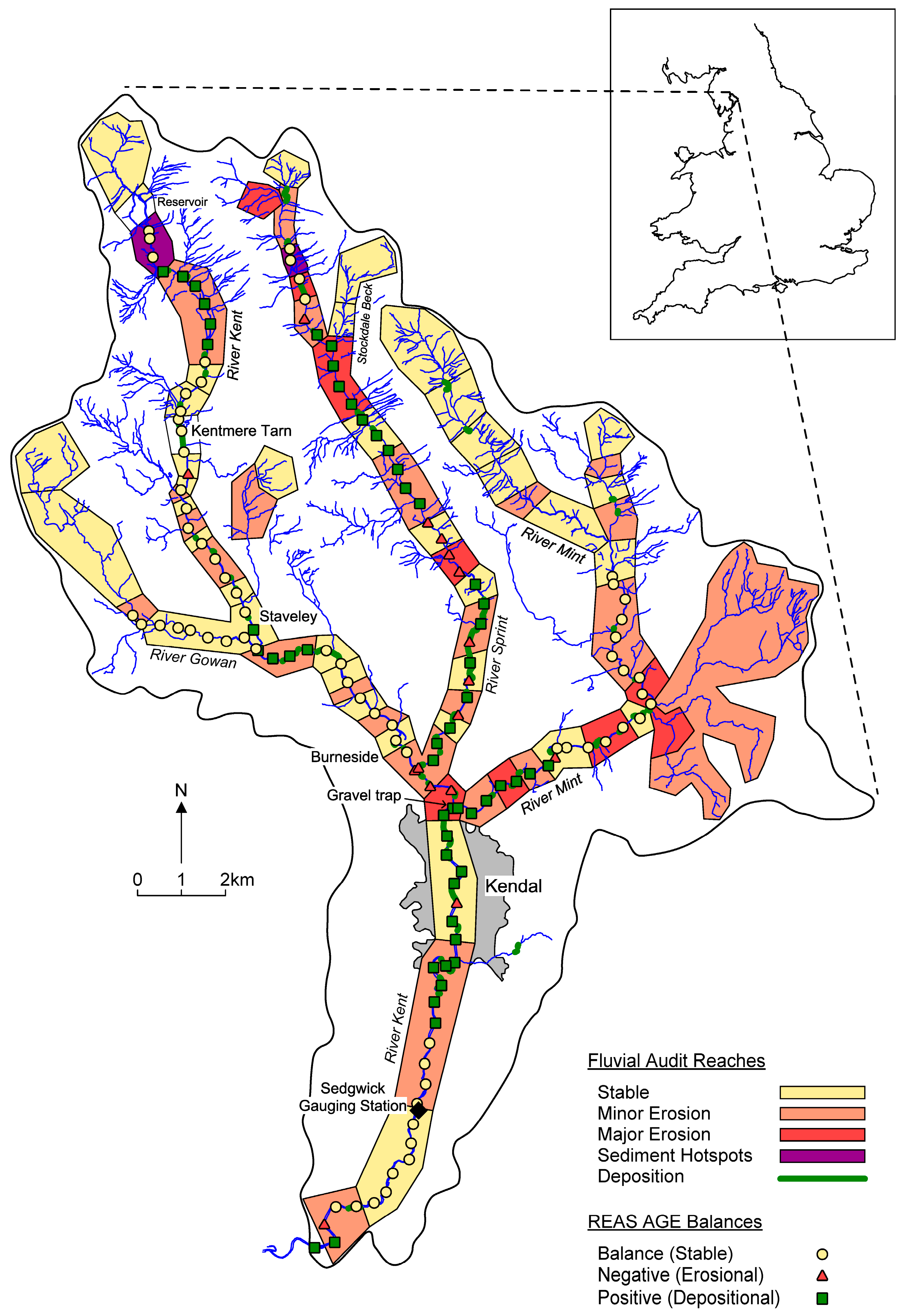
The River Kent rises in the south of the Lake District National Park, in the north-west of England, passes through the town of Kendal and outfalls into the Irish Sea at Heversham with a drainage basin area of approximately 225 km2 (inset Figure 1). The geology of the upper and middle drainage basin comprises Silurian slates and gritstones, whereas below Kendal the solid geology is limestone which outcrops in many places within the active channel. The landscape of the Kent basin is characterised by its glacial legacy but has been interwoven by artefacts of its recent industrial history, particularly mining activity in the upper reaches, water mills and their associated weirs in the middle and lower reaches and agricultural land drainage within the lower areas of the Sprint and Mint tributary watersheds. River terraces, glacial landforms and flood embankments act to inhibit lateral migration along several sections of its length and bedrock acts as a natural check on bed slope adjustment. During the 1970s, flood defence works were completed upstream of and through the town of Kendal, comprising channel widening, some realignment, flood retention walls and the construction of a gravel trap upstream of the town. Since the construction of these defences the Environment Agency has periodically removed coarse sediment deposits from the Kendal reach to maintain the design flood capacity.
In 2000, a Fluvial Audit was completed for the Kent basin [188] and revealed that the sediment transfer system in the River Kent and its main tributaries, the Gowan, Sprint and Mint (which join the Kent upstream of Kendal), is complex and comprises multiple sediment source, transfer and storage reaches. Bed incision, mining waste and inputs from tributaries provide a supply of coarse sediment and bank erosion and runoff from agricultural areas provide injections of finer sediment, enhanced by the close coupling of the channel with the upland terrain. Numerous sediment sinks are located at intermediate points along the river including gravel traps, natural lakes and mill ponds which interrupt the transfer of coarse sediment through the system. Consequently, it has been hypothesised by Wallerstein [189] that coarse sediments deposited in the flood control channel through Kendal are likely to be sourced locally in the reaches immediately upstream on the Kent, Sprint and Mint, rather than from headwater sources. The authors completed a revised Fluvial Audit characterisation of sediment sources, transfers and sinks along the River Kent [189], excluding tributaries, and although several discrepancies were identified, it generally corroborated the findings of the earlier report made by Orr et al. [188] for many reaches.
With a relatively complex sediment transport system, a history of flood risk management in Kendal and availability of a comprehensive Fluvial Audit, the River Kent basin provides a useful, albeit challenging, test case for the river energy auditing scheme developed here.
3.2. Application
Existing channel survey information exists for a significant length of the River Kent from the village of Kentmere in the headwaters to the village of Sedgwick in the lower course. However, this dataset does not cover the entire drainage basin, with significant deficiencies for the Gowan, Sprint and Mint tributaries. In light of this and with a view to testing REAS with only limited field data availability (for the general case) where a new comprehensive survey would be too expensive to commission and too time-consuming to complete for most projects, a new dataset was applied comprising 137 cross-sections spaced at approximately 500 m intervals, by employing the MAT software developed by JBA Consulting to the basin-wide LiDAR DEM (other comparable tools could have been applied). This ensured that the scheme covered the entire drainage basin for all ‘Main River’, designated by the Environment Agency. Where possible, sections were sited away from bridges and other structures or features where local hydraulics, slope adjustments and channel geometries could misrepresent the broader reach-scale trend. To reduce uncertainty, the existing survey data were used as control points in MAT (and in practice, verification would be undertaken through a number of targeted field visits).
A flow duration relationship was established from the flow record of the Sedgwick gauging station, located south of Kendal, comprising 40 years of mean daily discharges. A synthetic flow duration curve was then developed for each cross-section in the scheme scaled on the ratio of contributing drainage basin area to the area at the gauging station. The most demanding element of the data collection was obtaining and processing bed material sample data for computing the critical specific stream power for each cross-section (via interpolation). A total of 44 samples were retrieved at accessible locations (including two samples on the River Gowan and three samples on both the River Sprint and River Mint), considered to strike a balance between basin coverage and available resources without embarking on a lengthy and expensive data collection campaign that would not be feasible for most projects.
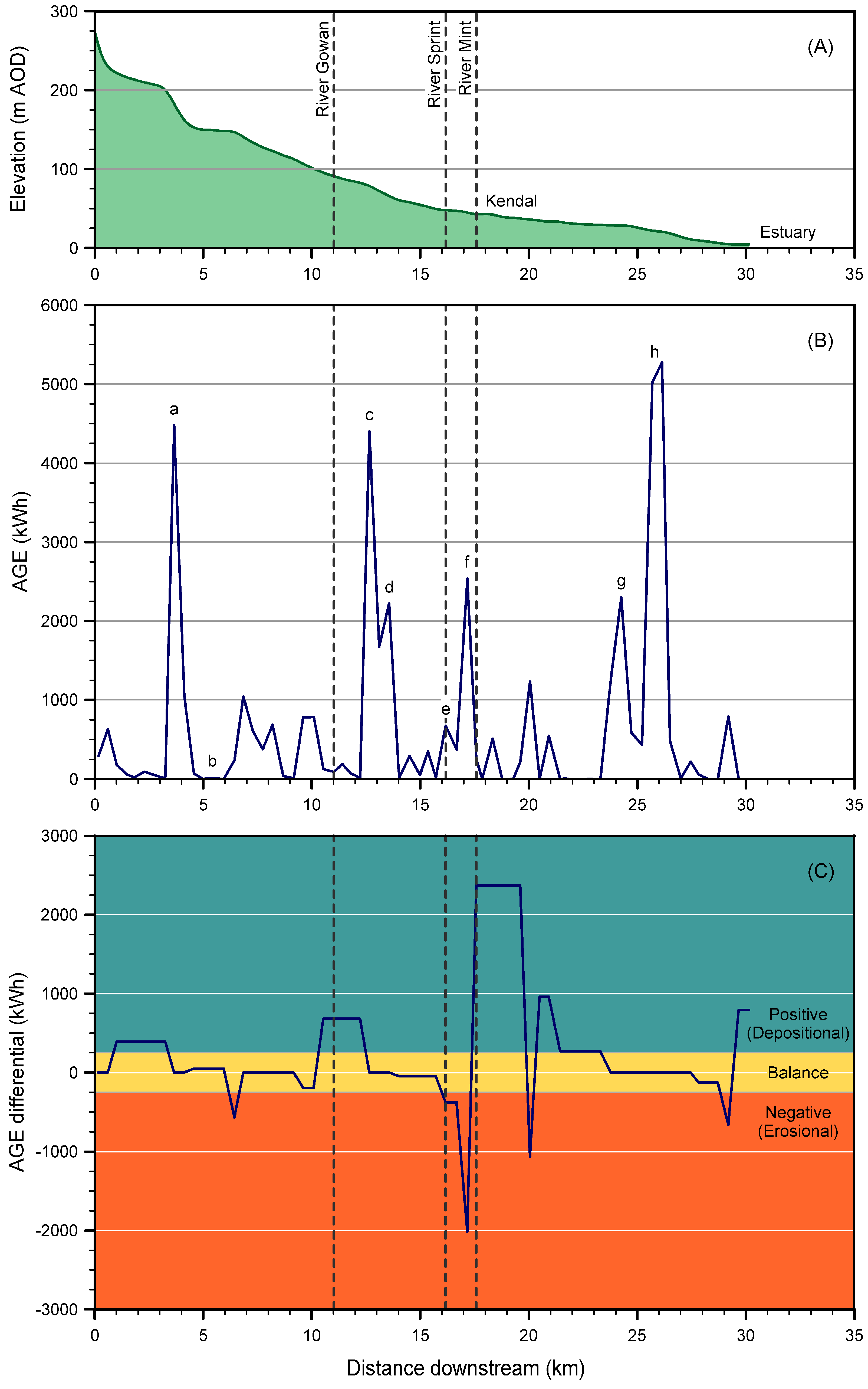
A baseline auditing scheme was established, suitable for providing a cost-effective screening of the drainage basin. The REAS results are compared with the results of the Fluvial Audit in Figure 1 and Figure 3, with Figure 2B,C displaying the downstream variation in Annual Geomorphic Energy (AGE) values and differentials, respectively, for each cross-section on the longitudinal profile (Figure 2A) of the main stem of the River Kent.
Some interesting features can be observed in the results. The main AGE peaks generally correspond to bedrock reaches (labelled a, c, d, g, h in Figure 2B) which are characteristically steeper than neighbouring reaches and, therefore, act as sediment transfer reaches with little potential for either progressive erosion of deposition. The peak labelled ‘a’ represents a steep bedrock gorge where the Kent plunges from a hanging valley through the village of Kentmere and down to Kentmere Tarn. The Tarn, denoted by the trough labelled ‘b’, acts as a natural sediment trap. Peaks ‘c’ and ‘d’ correspond to a confined reach downstream of Staveley where slope is controlled to a degree by outcrops of metamorphic bedrock. The minor peak labelled ‘e’ corresponds approximately to the location of the Burneside paper mill weir (a location where the REAS results appear to have been influenced marginally by a local artificial control on sediment dynamics) and the significant peak labelled ‘f’ corresponds to a short meandering reach upstream of the Mint confluence and gravel trap where the bed slope was observed to steepen slightly before flattening out at the Mint confluence. Peaks ‘g’ and ‘h’ are attributable directly to discontinuities in bed slope as the river passes over exposed, flat-bedded limestone with notable waterfalls and locally steep reaches. Of note is the slightly convex bed profile between Kendal and the estuary near Heversham which is related to the outcrops of limestone. The presence of these high-energy spikes and deviation from an idealised graded longitudinal profile are not unsurprising as the Kent drainage basin has a characteristically interrupted sediment transfer system.
The presence of steep bedrock reaches could yield misleading results, indicating potential for degradation followed by aggradation immediately downstream. In light of this, and following field visits to substantiate the decision, these locations were set as fixed sediment ‘transfers’ in REAS. This type of refinement is similar to selecting the ‘hard bed’ option in the iSIS Sediments software for cross-sections, where the bed is not permitted to scour when running the model (although in iSIS, deposition can still occur). In general, the authors found no evidence of substantial deposition within the bedrock reaches of the Kent basin that could be described as aggradation, although the Fluvial Audit reveals some bedrock areas with temporary storage features. In between the bedrock locations, however, reaches of sediment deposition are not uncommon with values of AGE rarely exceeding 500 kWh, including the River Kent through the Kendal flood alleviation scheme.
The AGE differentials based on Equation (8) are illustrated in Figure 2C. Where there are known bedrock outcrops, the AGE differentials are set to zero, reflecting potential for sediment transfer only. Examination of the differentials calculated for individual cross-sections reveals considerable variability over short distances in the available energy for performing geomorphological work, reflecting the characteristic local variability in bed slope, cross-sectional geometry and bed-sediment composition. The main zone of activity is concentrated near the Sprint and Mint confluences, suggesting the potential for erosional processes near the Sprint confluence followed by short reaches of depositional and erosional tendencies before the Mint confluence and the location of the gravel trap, where the results clearly indicate potential for sediment deposition.
The influence of the global zonation algorithm (see Section 2.2.3) on the REAS results is two-fold. First, there is less variability overall and second, there are extended reach lengths of positive differential (indicative of sediment deposition) at the Gowan confluence and, notably, downstream of the Mint confluence and through Kendal. The global zonation algorithm assigned cross-sections with similar AGE values to distinct reaches, such that the total of the reach variances was only approximately one percent of the global variance for all cross-sections. Importantly, the results refer only to imbalances in available energy and there is a risk of misinterpretation in their association with sediment transport processes at locations where channel stability status is controlled by the many local factors not accounted for in the long-stream distribution of stream power. Despite this caution, though, deposition has been reported at numerous locations throughout Kendal and Orr et al. [188] considered the town to be the main depositional area, with 8025 tonnes of material removed from various sites between 1991 and 2000, even with the upstream gravel trap in close proximity. Depositional features were also reported in the Fluvial Audit downstream of the Gowan confluence, although these were not sufficiently extensive to suggest aggradation.
In Figure 1, specifying a tolerance value of AGE differential for the Kent drainage basin that would define equilibrium conditions in terms of sediment transfer is not straightforward. In the absence of any guidance or previous applications, an arbitrary value of ±250 kWh was chosen as it accounted for the low amplitude variability in cross-section differentials, assumed to be attributed to natural variability in sediment transfer rather than channel instability. Of course, the distribution of positive and negative AGE differentials could be very sensitive, in some cases, to the choice of tolerance value and deciding on a final value (if needed) should be exercised with caution.
Figure 1 illustrates the following AGE balance (differential) categories:
- Balance (indicative of stability or equilibrium in sediment transfer);
- Negative (indicative of the potential for erosional processes), and;
- Positive (indicative of the potential for depositional processes).
Orr et al. [188] defined five main categories for the Fluvial Audit results:
- Stable (grouping three sub-categories);
- Minor erosion (mainly washout around trees);
- Extensive active erosion (defined here as ‘major erosion’);
- Sediment hotspot (major management issue), and;
- Deposition (although no reaches were defined as entirely depositional).
Two sediment hotspots were defined for the upper Kent and Sprint as areas of major reworking of sediment with a history of incision following significant inputs of mining waste. These two areas are considered by Orr et al. [188] to be major sources of sediment within the catchment but it is immediately apparent that mining waste mobilised in the headwaters of the River Kent cannot be associated with observed sedimentation in the lower Kent reaches as Kentmere Tarn acts as an efficient natural sediment trap.
There are areas of both similarity and difference between the REAS and Fluvial Audit results (Figure 3). Critically, some of the differences can be attributed to interpretation in the Fluvial Audit, for example reaches defined as minor erosion appear to exhibit generally stable bed and banks (when visited in the field), but with some discontinuous bank erosion between trees (as found in many geomorphologically stable channels and not necessarily indicative of instability). Importantly, erosion that is reported in the Kent Fluvial Audit generally refers to bank erosion and not bed scour, and is mainly attributable to cattle poaching and where bank strength has been reduced through loss of vegetation cover [188]. The REAS approach, in contrast, reveals discontinuities in energy only as ‘indicative’ of locations of potential geomorphic activity and does not accommodate lateral influences such as bank erosion, sediment runoff or the input of other sediment sources such as mining waste. As such, REAS might identify an area with stable energy conditions, although the channel might be exhibiting deposition due to non-channel sediment inputs. For negative (erosional) REAS AGE balances, Figure 3A reveals a reasonable agreement (60 percent) between the two methods. Parity between stable sites is over 50 percent and if assigning wider interpretation to Fluvial Audit minor erosion sites, as discussed above, conceivably accordance might increase to over 85 percent. Interestingly, positive (depositional) REAS AGE balances are distributed over both stable and erosional Fluvial Audit reaches, but with a propensity to lie within broadly erosional reaches, thus confirming a general pattern of juxtaposed erosional and depositional geomorphological activity within the drainage basin as a whole while also illustrating the wider challenges of demarcating reaches in the Fluvial Audit method and process-based classification in watershed assessments more generally. With no Fluvial Audit reaches classified as entirely depositional, Figure 3B reveals that almost a quarter of REAS cross-sections with positive AGE balance (depositional) are sited directly within depositional sub-areas in the Fluvial Audit, rising to 50 percent of cross-sections within 175 m of the nearest depositional sub-area and 75% within 300 m.
The main areas of disagreement between the two methods possibly reflect the non-accounting of lateral sediment transfers and exchanges. Examples of these areas in Figure 1 include the upper reaches of the River Kent (below the reservoir), the upper reaches of the River Sprint through the confluence with Stockdale Beck and some of the middle to lower reaches of the River Mint (although some depositional areas were also recorded here within a largely erosional zone in the Fluvial Audit). Further field visits would be necessary to investigate the extent to which the reported eroding banks are coupled with marked deposition features. Other disagreements, particularly where REAS indicates potential for deposition, are possibly attributed to discontinuity in sediment transfer associated with numerous weirs that act to trap sediment, preventing material from being transferred and deposited further downstream, but are not accounted for at the basin scale of analysis inherent to REAS. Conversely, there are many locations where the two approaches show degrees of consistency, especially if the minor erosion reaches in the Fluvial Audit are considered to be stable at the system scale. For example, Figure 1 illustrates areas of agreement on the River Kent immediately upstream of Kentmere Tarn, for the majority of the stable reach between Kentmere Tarn and Staveley, along a considerable stable reach upstream of Burneside, at a zone of erosion along the lower reach of the River Kent, at a zone of major erosion in the middle course of the River Sprint followed by a length of deposition (although within a reach classified as minor erosion in the Fluvial Audit), within several of the middle reaches of the River Mint and for the stable lower reaches of the River Gowan.
There are a number of other features in Figure 1 that are worthy of note. Kentmere Tarn is shown in the REAS map to be in energy equilibrium, suggestive of a morphologically stable rather than indicative of depositional processes, which reflects the inability to account for the sediment trapping function of the lake. The only location of negative AGE differential (erosional processes) on the River Mint is shown to lie within a stable Fluvial Audit reach. Closer inspection of the dataset reveals that there is a significant, local increase in bed slope downstream of two meander bends at a location known as Meal Bank. It is uncertain whether the bed at this location comprises alluvial material, with potential through scour to supply sediment to the lower reaches and the River Kent, or if bedrock is present and material is transferred through. A further point of interest is the match between the negative AGE balance and the erosional reach in the Fluvial Audit between the Sprint and the Mint confluences, which coincides in the REAS dataset with a moderate steepening of bed slope. Despite this agreement, though, inspection during a field visit [189] revealed no discernible channel instability near the Sprint confluence (possibly due to the weir sited at the Burneside paper mill, which has acted to stabilise the bed), or in the meandering reach upstream of the gravel trap at the Mint confluence (although there is extensive bank erosion where the banklines are unprotected, as highlighted in the Fluvial Audit report). The meandering reach exhibits a gradual flattening of bed slope towards the gravel trap.
The AGE values through Kendal exhibit relatively low variability, hence the extension of the REAS reach of positive AGE balance (depositional) through the town (according to the global zonation algorithm for delineating reaches). Although the Fluvial Audit designated the urban reach as geomorphologically stable, the report also clearly highlights that Kendal is a major depositional zone, as indicated by the deposition locations shown in Figure 1. Sediment tends to accumulate in Kendal in the vicinity of bridge piers and weirs, such as Stramongate Weir, and where the channel locally widens. While these sediment accumulations might present an increased flood risk if not removed periodically, it remains unclear as to whether the features are a result of local scour and fill processes rather than a consequence of instability at the basin scale.
4. Discussion and Conclusions
With the increasing acknowledgement between practitioners that river and flood risk management activities should take into account the transport of sediment in river channels, geomorphologists are faced with the challenge of identifying existing methods and developing new strategic level approaches that can characterise disconnections in sediment transfer at the basin scale and highlight locations or reaches where more detailed analysis and resources should be targeted. In meeting this objective, approaches must balance science with pragmatism if they are to have utility value and be employed routinely, as well as credible theoretical and methodological underpinnings, even if this means accepting a level of uncertainty that might not normally be satisfactory in blue sky academic research. A River Energy Audit Scheme, REAS, has been explored here as one possible tool for achieving this, by characterising the potential for a river to perform geomorphological work revealed in a measure of stream Annual Geomorphic Energy differential and using this accounting system to infer conditional sediment transfer dynamics. The term ‘conditional’ is critical here in that energy balance might not always correlate with sediment balance and propensity for morphological change through erosion or deposition (a conclusion also of Lea and Legleiter [2]) and this will remain a limitation of any energy-based approach.
The discordance between the energy budget and river channel stability status is a function of the multitude of controls on sediment transport that do not feature in stream power calculations, including sensitivity of the channel boundary to change (and relative sensitivities between bed and banks), sediment supply limitations, structures that disrupt sediment continuity beyond the local scale, channel evolution/recovery (or indeed non-recovery following the most extreme flood events) in response to recent or historical influences (extrinsic or autogenic) and sediment sources associated with bank erosion, planform change and runoff. In terms of lateral instability, Buraas et al. [184] made some headway by demonstrating how widening and large scale geomorphic change relate to crossing a threshold specific stream power (for the 2-year flow) of 300 W·m−2 during flood events, which facilitated a regional assessment of reaches susceptible to bank erosion. Conceivably then, it would be possible to estimate the proportion of AGE that might be associated with large scale bank retreat and map susceptible reaches.
While in many cases the contribution to the channel-forming bed material load made by non-channel sediment sources might be judged to be minor, in some environments a significant proportion of the load imposed upon the channel is derived from the drainage basin itself [190]. Such a case may be found where floodplains composed of erodible soils have been considerably modified by arable agriculture or where a stream is closely coupled to steep hill slopes with significant injections of colluvial material. In addition, the annual load of eroded bank material cannot readily be quantified in terms of the dissipation of available energy or stream power within the channel and remains an unresolved issue. Thus, where there are zones of significant non-channel sediment inputs, the link between energy balance and reaches of sediment source, transfer and sink identified in a qualitative basin-wide assessment (such as the Fluvial Audit) might for some cases be tenuous at best. While in such cases auditing stream power might present an overly reductionist picture of channel stability, the outcomes then will only have utility value if follow-up investigations concentrate on potential reaches of concern that only become validated based on other supporting information. In examining disparities between the REAS results and the Fluvial Audit map of reaches, the case study revealed how local controls, such as weirs, appear to be accounted for by the Fluvial Audit (e.g., sediment trapping) but do not have the same influence at the basin scale of analysis inherent to REAS (unless modifying the broad channel gradient). Inevitably, therefore, there is likely to be some disagreement between these two types of approach and in bringing together their respective findings, disparities should not necessarily be treated as errors because the two treatments are potentially providing ‘complementary’ rather than ‘contradictory’ evidence to the river manager. Thus, the overall merit of such an energy-based approach is in screening the river network to flag potential issues (that may or may not become realised) as a supporting tool and should not be recommended as the replacement for other types of geomorphological assessment.
In addition to data interpretation, there remain several sources of uncertainty related to issues of data quality and data processing. The collation of input data at the basin-wide scale for processing in the stream power calculations is affected by the availability of information, the necessary coarseness of sampling needed at this scale and, critically, whether data acquired are indeed representative of the reaches they relate to with acceptable accuracy. With results of the method expressed as ‘annualised’ quantities, assuming stationarity in the input data, e.g., bed material gradation, for a system with geomorphologically unstable reaches might be construed as a potential source of uncertainty.
Additional sources of uncertainty are associated with the measurement of channel dimensions and slope, the collection of sediment data, assignment of roughness values and synthesis of hydrological data. As slope here represents average energy condition within a reach, it is considered in most cases that bed slope or even valley slope are suitable parameters at the coarse scale the methodology is applied. With the availability of flow and sediment size information likely to be very limited, some degree of interpolation within the project catchment is unavoidable as a lengthy field campaign to collect detailed inventories of data are unlikely to be feasible in most cases.
The types of data available will be dictated by their costs, processing times and licensing agreements, with collection of cross-section survey information a particularly costly component of many river projects. During the data processing stage, sources of uncertainty manifest through the assumptions and approximations made within the equations themselves. These include the choice of the Shields entrainment coefficient (0.045) and selection of the hiding function in Ferguson’s [131] reworking of Bagnold’s expression for critical stream power, and the calculation and partitioning of discharge using the Manning equation. Conceivably, through repeated runs of REAS and by adjusting input data values within sensible ranges, uncertainty-bounded estimates of AGE could be derived and mapped to reveal the extent to which the distribution of REAS reaches is sensitive to the data inputs. It is also pertinent to note at this point that no account is made here for the potential loss in conveyance, and therefore stream power, associated with the lateral exchange in momentum between channel and floodplain flows. While empirically-based methods are available for accounting for this source of energy dissipation (e.g., [191,192]), they are considered to be beyond the scope of a basin-scale auditing scheme (and indeed are omitted from one-dimensional hydraulic modelling packages, such as HEC-RAS).
One of the greatest sources of uncertainty is in the identification of unique reaches of energy similarity for calculating the differentials in AGE. The methods described here provide solutions but are not without their problems. In particular, the global zonation algorithm can define a long reach comprising many cross-sections as a positive energy differential (and thus indicative of depositional processes), whereas in reality it is perhaps more likely that deposition would occur for only a short distance near the head of the reach. Reach delineation methods can, therefore, artificially propagate instability effects and results should be interpreted taking into account this potential process-response misalignment (especially when drawing direct at-a-site comparisons between the results from REAS and field-based assessments). In addition, the choice of threshold absolute AGE differential necessary to demarcate geomorphologically stable reaches is not straightforward (an issue also considered in other basin-wide assessment methods [118,123]) and its somewhat subjective setting might hold significance when applying REAS across different types of river system. In light of the above issues a degree of uncertainty is, therefore, an inevitable outcome of the energy balance approach and should not necessarily be treated as a limitation at this broad scale of analysis.
The rapid development of automated tools for basin-wide hydro-geomorphic assessment, coupled with the proliferation of accessible regional and national datasets are enabling channel geometries, bathymetric surveys, longitudinal profiles and bed material gradations to be derived on a routine basis across the river science community. At the basin scale, technological advances in the use of remote sensing (for reviews see [193,194,195,196,197,198]), assembly and computer management of big datasets and feature-based image processing procedures are collectively facilitating a revolutionary movement in geospatial mapping [150,199] with considerable potential for supporting basin-wide studies on flood risk, sediment transfer, morphological and habitat characterisation and river management that have been unfeasible in the past from field-based assessments alone [143,200]. In contrast, over-reliance on field-based data to inform basin-wide assessments can be costly, resource intensive, hazardous and risks incomplete coverage [34], especially for tributaries. With the emerging study of ‘digital’ rivers, with large scale continuous datasets and increasingly less reliance on field-based analyses of point data, stream power calculations are thus becoming ever more achievable and cost-effective in the assimilation of basin-wide databases to inform river management. Integrated tools are now available, such as the ArcGIS toolboxes FluvialCorridor [201] and RESonate [202] and the IDRAIM framework for fluvial characterisation [203,204], and they will continue to be developed and refined to reflect emerging technologies, the growth of data sources and widening applications. Although costly, limited in coverage and associated with operational issues, field-based methods are still invaluable in providing complementary and supplementary data [141,205], notably for calibrating remotely sensed and image-processed datasets. Conceivably then, big hydro-geomorphic data capture and automated feature extraction methods are poised to provide the quantitative framing to the Fluvial Audit as a realistic near term prospect and thus a more objective basis to strategic planning, resource prioritisation and sustainable management practices.
This research has demonstrated that successful employment of an energy-based auditing scheme would depend in part on marrying the methodology with a companion guide to decision making, data collection alternatives and processing stages, listing their respective merits and pitfalls in supporting basin-scale assessments. For example, further consideration must be given to deriving channel slope, the spatial scale over which it should be determined, how best to avoid local variability in bed elevations and acceptable bounds of uncertainty.
In conclusion, this research has provided a conceptual platform for further development and testing and, importantly, it has made an insightful contribution to the drive towards integrating fluvial geomorphology in river channel and flood risk management. Characterising sediment transfer in terms of energy budgeting is an innovative technique, conceptually, that focuses on fluvial drivers, in this case available energy that the river can dispense on generating geomorphological activity, rather than predicting fluvial morphology, per se. The practical utility value of this type of approach, therefore, lies in the careful interpretation of the results as ‘indicative’ only in the context of assumptions made, with an understanding of the broad-scale methodology applied and with an appreciation of the above limitations and potential sources of uncertainty. Despite these points, the scheme presented does not over-caricature the sediment transfer system but rather makes a valid attempt to synthesise potential geomorphological responses. An initial test application in the River Kent suggests that the methodology has merit, although it cannot entirely replace field-based methods of geomorphological enquiry and should be treated as a complementary mode of analysis to be performed alongside other methods selected from the available range of approaches. The overall premise of being a practical and robust approach will always present a challenge for reducing the level of uncertainty, compounded by its discrete, rather than systemic, treatment of geomorphological reaches that have no influence beyond their immediate neighbours. However, the future prospect is that basin-scale methods will no longer have to be light on data requirements—which is potentially paradigm-shifting in system-wide geomorphological assessment.
Acknowledgments
This research was partly conducted through the Flood Risk Management Research Consortium (FRMRC Phase 1), under Work Package 8.2: ‘Morphology, Sediments and Habitats’. The principal sponsor for the project was the Engineering and Physical Sciences Research Council under grant GR/S76304/01, with additional contributions from the Natural Environment Research Council, Defra and the Environment Agency through their joint R&D programme on Flood and Coastal Defence, the Scottish Executive, the Rivers Agency (Northern Ireland) and UK Water Industry Research. The authors are grateful to three anonymous reviewers for their constructive comments for improving the manuscript. This paper reflects the authors’ views only and not those of the FRMRC funding organisations or partners.
Author Contributions
Philip J. Soar, Nicholas P. Wallerstein and Colin R. Thorne conceived the River Energy Audit Scheme and designed the programme of research; Philip J. Soar and Nicholas P. Wallerstein performed the analyses; Philip J. Soar wrote the paper; Nicholas P. Wallerstein and Colin R. Thorne provided editorial improvements to the paper.
Conflicts of Interest
The authors declare no conflict of interest. The founding sponsors had no role in the design of the study, in the collection, analyses, or interpretation of data, in the writing of the manuscript and in the decision to publish the results.
References
- Downs, P.W.; Gregory, K.J. River Channel Management: Towards Sustainable Catchment Hydrosystems; Arnold: London, UK, 2014. [Google Scholar]
- Lea, D.M.; Legleiter, C.J. Mapping spatial patterns of stream power and channel change along a gravel-bed river in northern Yellowstone. Geomorphology 2016, 252, 66–79. [Google Scholar] [CrossRef]
- Thorne, C.R.; Soar, P.J.; Skinner, K.S.; Sear, D.A.; Newson, M.D. Driving processes II. Investigating, characterising and managing river sediment dynamics. In Guidebook of Applied Fluvial Geomorphology; Sear, D.A., Newson, M.D., Thorne, C.R., Eds.; Thomas Telford: London, UK, 2010; pp. 120–195. [Google Scholar]
- Thorne, C.R.; Wallerstein, N.P.; Soar, P.J.; Brookes, A.; Duncan, W.; Biedenharn, D.S.; Gibson, S.A.; Little, C.D.; Mooney, D.M.; Watson, C.C.; et al. Accounting for sediment in flood risk management. In Flood Risk Science and Management; Pender, G., Faulkner, H., Eds.; Wiley-Blackwell: Oxford, UK, 2011; pp. 87–113. [Google Scholar]
- Lane, E.M. The importance of fluvial morphology in hydraulic engineering. Am. Soc. Civ. Eng. Proc. Sep. 1955, 81, 1–17. [Google Scholar]
- Schmidt, J.C.; Wilcock, P.R. Metrics for assessing the downstream effects of dams. Water Resour. Res. 2008, 44, W04404. [Google Scholar] [CrossRef]
- Darby, S.E.; Rinaldi, M.; Dapporto, S. Coupled simulations of fluvial erosion and mass wasting for cohesive river banks. J. Geophys. Res. Earth Surf. 2007, 112. [Google Scholar] [CrossRef]
- Stover, S.C.; Montgomery, D.R. Channel change and flooding, Skokomish River, Washington. J. Hydrol. 2001, 243, 272–286. [Google Scholar] [CrossRef]
- Raven, E.K.; Lane, S.N.; Ferguson, R.I.; Bracken, L.J. The spatial and temporal patterns of aggradation in a temperate, upland, gravel-bed river. Earth Surf. Process. Landf. 2009, 34, 1181–1197. [Google Scholar] [CrossRef]
- Bullen Consultants Ltd. Glossop Brook Flood Event Appraisal: 30 July 2002 Flood Event; Bullen Consultants Ltd.: Birkenhead, Merseyside, UK, 2003; p. 46. [Google Scholar]
- Department of the Environment. The Occurrence and Significance of Erosion, Deposition and Flooding in Great Britain; Department of the Environment: London, UK, 1995; p. 178.
- Sear, D.A.; Newson, M.D.; Brookes, A. Sediment-related river maintenance: The role of fluvial geomorphology. Earth Surf. Process. Landf. 1995, 20, 629–647. [Google Scholar] [CrossRef]
- Newson, M.D. Geomorphic thresholds in gravel-bed rivers. In Dynamics of Gravel-Bed Rvers; Billi, P., Hey, R.D., Thorne, C.R., Tacconi, P., Eds.; John Wiley & Sons: Chichester, UK, 1992; pp. 3–15. [Google Scholar]
- Hooke, J. Coarse sediment connectivity in river channel systems: A conceptual framework and methodology. Geomorphology 2003, 56, 79–94. [Google Scholar] [CrossRef]
- Biedenharn, D.S.; Thorne, C.R.; Watson, C.C. Recent morphological evolution of the Lower Mississippi River. Geomorphology 2000, 34, 227–249. [Google Scholar] [CrossRef]
- Booth, D.B.; Fischenich, C.J. A channel evolution model to guide sustainable urban stream restoration. Area 2015, 47, 408–421. [Google Scholar] [CrossRef]
- Soar, P.J.; Thorne, C.R. Channel Restoration Design for Meandering Rivers; ERDC/CHL Report CR-01-1; U.S. Army Corps of Engineers Engineer Research & Development Center: Vicksburg, MS, USA, 2001; p. 429. [Google Scholar]
- Pollock, M.M.; Beechie, T.J.; Wheaton, J.M.; Jordan, C.E.; Bouwes, N.; Weber, N.; Volk, C. Using beaver dams to restore incised stream ecosystems. Bioscience 2014, 64, 279–290. [Google Scholar] [CrossRef]
- Shields, F.D.J.; Doyle, M.W. Sedimentation engineering design in river restoration: System stability assessment for design guidance. In Proceedings of the 1999 International Water Resources Engineering Conference, Seattle, WA, USA, 8–12 August 1999; Walton, R., Nece, R.E., Eds.; Environmental and Water Resources Institute of the American Society of Civil Engineers: Reston, VA, USA, 1999. [Google Scholar]
- Dust, D.; Wohl, E. Conceptual model for complex river responses using an expanded Lane’s relation. Geomorphology 2012, 139–140, 109–121. [Google Scholar] [CrossRef]
- Huang, H.Q.; Liu, X.; Nanson, G.C. Commentary on a “Conceptual model for complex river responses using an expanded Lane diagram by David Dust and Ellen Wohl”. Geomorphology 2014, 209, 140–142. [Google Scholar] [CrossRef]
- Kiraga, M.; Popek, Z. Using a modified Lane’s relation in local bed scouring studies in the laboratory channel. Water 2016, 8, 16. [Google Scholar] [CrossRef]
- Harvey, A.M. Effective timescales of coupling within fluvial systems. Geomorphology 2002, 44, 175–201. [Google Scholar] [CrossRef]
- Brierley, G.; Fryirs, K.; Jain, V. Landscape connectivity: The geographic basis of geomorphic applications. Area 2006, 38, 165–174. [Google Scholar] [CrossRef]
- Bracken, L.J.; Croke, J. The concept of hydrological connectivity and its contribution to understanding runoff-dominated geomorphic systems. Hydrol. Process. 2007, 21, 1749–1763. [Google Scholar] [CrossRef]
- Raven, E.K.; Lane, S.N.; Bracken, L.J. Understanding sediment transfer and morphological change for managing upland gravel-bed rivers. Prog. Phys. Geogr. 2010, 34, 23–45. [Google Scholar] [CrossRef]
- Fryirs, K. (Dis)Connectivity in catchment sediment cascades: A fresh look at the sediment delivery problem. Earth Surf. Process. Landf. 2013, 38, 30–46. [Google Scholar] [CrossRef]
- Koiter, A.J.; Owens, P.N.; Petticrew, E.L.; Lobb, D.A. The behavioural characteristics of sediment properties and their implications for sediment fingerprinting as an approach for identifying sediment sources in river basins. Earth Sci. Rev. 2013, 125, 24–42. [Google Scholar] [CrossRef]
- Bracken, L.J.; Turnbull, L.; Wainwright, J.; Bogaart, P. Sediment connectivity: A framework for understanding sediment transfer at multiple scales. Earth Surf. Process. Landf. 2015, 40, 177–188. [Google Scholar] [CrossRef] [Green Version]
- Schmitt, R.J.P.; Bizzi, S.; Castelletti, A. Tracking multiple sediment cascades at the river network scale identifies controls and emerging patterns of sediment connectivity. Water Resour. Res. 2016, 52, 3941–3965. [Google Scholar] [CrossRef]
- Downs, P.W.; Dusterhoff, S.; Leverich, G.; Soar, P.J.; Napolitano, M. Structured insights into Anthropocene fluvial system dynamics evidenced through sediment budget analysis of a highly regulated catchment. Earth Surf. Process. Landf. 2017. under review. [Google Scholar]
- Wohl, E.; Bledsoe, B.P.; Jacobson, R.B.; Poff, N.L.; Rathburn, S.L.; Walters, D.M.; Wilcox, A.C. The natural sediment regime in rivers: Broadening the foundation for ecosystem management. Bioscience 2015, 65, 358–371. [Google Scholar] [CrossRef]
- Iacob, O.; Rowan, J.S.; Brown, I.; Ellis, C. Evaluating wider benefits of natural flood management strategies: An ecosystem-based adaptation perspective. Hydrol. Res. 2014, 45, 774–787. [Google Scholar] [CrossRef]
- Newson, M.D.; Large, A.R.G. “Natural” rivers, “hydromorphological quality” and river restoration: A challenging new agenda for applied fluvial geomorphology. Earth Surf. Process. Landf. 2006, 31, 1606–1624. [Google Scholar] [CrossRef]
- Wallerstein, N.P.; Thorne, C.R.; Soar, P.J.; Brookes, A.; Biedenharn, D.S.; Watson, C.C.; Gibson, S.; Little, C.; Mooney, D.; Green, A.P.; et al. Accounting for Sediment in Rivers: A Tool Box of Sediment Transport and Transfer Analysis Methods and Models to Support Hydromophologically-Sustainable Flood Risk Management in the UK; Flood Risk Management Research Consortium, University of Nottingham: Nottingham, UK, 2006; p. 134. [Google Scholar]
- Environment Agency. River Geomorphology: A Practical Guide; Guide Note 18; Environment Agency: Bristol, UK, 1998; p. 56. [Google Scholar]
- Sear, D.; Newson, M.; Hill, C.; Old, J.; Branson, J.A. method for applying fluvial geomorphology in support of catchment-scale river restoration planning. Aquat. Conserv. Mar. Freshw. Ecosyst. 2009, 19, 506–519. [Google Scholar] [CrossRef]
- Thorne, C.R.; Soar, P.J.; Skinner, K.S. Characterising and managing river sediment dynamics. In Guidebook of Applied Fluvial Geomorphology; Sear, D.A., Thorne, C.R., Newson, M.D., Eds.; Thomas Telford: London, UK, 2010; pp. 120–195. [Google Scholar]
- Johnson, P.A. Preliminary assessment and rating of stream channel stability near bridges. J. Hydraul. Eng. 2005, 131, 845–852. [Google Scholar] [CrossRef]
- Johnson, P.A.; Whittington, R.M. Vulnerability-based risk assessment for stream instability at bridges. J. Hydraul. Eng. 2011, 137, 1248–1256. [Google Scholar] [CrossRef]
- Cluer, B.; Thorne, C.R. A stream evolution model integrating habitat and ecosystem benefits. River Res. Appl. 2014, 30, 135–154. [Google Scholar] [CrossRef]
- Brierley, G.J.; Fryirs, K.A. Geomorphology and River Management: Applications of the River Styles Framework; Blackwell Publishing: Oxford, UK, 2005. [Google Scholar]
- Belletti, B.; Rinaldi, M.; Buijse, A.D.; Gurnell, A.M.; Mosselman, E. A review of assessment methods for river hydromorphology. Environ. Earth Sci. 2014, 73, 2079–2100. [Google Scholar] [CrossRef]
- Gomez, B.; Church, M. An assessment of bed load sediment transport formulae for gravel bed rivers. Water Resour. Res. 1989, 25, 1161–1186. [Google Scholar] [CrossRef]
- Wilcock, P.R. Toward a practical method for estimating sediment-transport rates in gravel-bed rivers. Earth Surf. Process. Landf. 2001, 26, 1395–1408. [Google Scholar] [CrossRef]
- Barry, J.J.; Buffington, J.M.; King, J.G. A general power equation for predicting bed load transport rates in gravel bed rivers. Water Resour. Res. 2004, 40, W10401. [Google Scholar] [CrossRef]
- Martin, Y.; Ham, D. Testing bedload transport formulae using morphologic transport estimates and field data: Lower Fraser River, British Columbia. Earth Surf. Process. Landf. 2005, 30, 1265–1282. [Google Scholar] [CrossRef]
- Papanicolaou, A.N.; Elhakeem, M.; Krallis, G.; Prakash, S.; Edinger, J. Sediment transport modeling review: Current and future developments. J. Hydraul. Eng. 2008, 134, 1–14. [Google Scholar] [CrossRef]
- Merritt, W.S.; Letcher, R.A.; Jakeman, A.J. A review of erosion and sediment transport models. Environ. Model. Softw. 2003, 18, 761–799. [Google Scholar] [CrossRef]
- Reaney, S.M.; Lane, S.N.; Heathwaite, A.L.; Dugdale, L.J. Risk-based modelling of diffuse land use impacts from rural landscapes upon salmonid fry abundance. Ecol. Model. 2011, 222, 1016–1029. [Google Scholar] [CrossRef]
- Coulthard, T.J.; Neal, J.C.; Bates, P.D.; Ramirez, J.; de Almeida, G.A.M.; Hancock, G.R. Integrating the LISFLOOD-FP 2D hydrodynamic model with the CAESAR model: Implications for modelling landscape evolution. Earth Surf. Process. Landf. 2013, 38, 1897–1906. [Google Scholar] [CrossRef]
- Biedenharn, D.S.; Hubbard, L.C.; Thorne, C.R.; Watson, C.C. Understanding Sediment Sources, Pathways, and Sinks in Regional Sediment Management: Application of Wash Load and Bed-Material Load Concept; Technical Notes TN-SWWRP-06-4; U.S. Army Corps of Engineers, Engineer Research & Development Center: Vicksburg, MS, USA, 2006; p. 12. [Google Scholar]
- Gibson, S.A.; Little, C.D. Implementation of the Sediment Impact Assessment Model (SIAM) in HEC-RAS. In Proceedings of the Eighth Federal Interagency Sedimentation Conference (8th FISC), Reno, NV, USA, 2–6 April 2006; pp. 65–72.
- Little, C.D.; Jonas, M. Sediment Impact Analysis Method (SIAM): Overview of model capabilities, applications, and limitations. In Proceedings of the 2nd Joint Federal Interagency Conference on Sedimentation and Hydrologic Modeling, Las Vegas, NV, USA, 27 June–1 July 2010.
- Wolman, M.G.; Miller, J.P. Magnitude and frequency of forces in geomorphic processes. J. Geol. 1960, 68, 54–74. [Google Scholar] [CrossRef]
- Andrews, E.D. Effective and bankfull discharges of streams in the Yampa River basin, Colorado and Wyoming. J. Hydrol. 1980, 46, 311–330. [Google Scholar] [CrossRef]
- Soar, P.J.; Thorne, C.R. Design discharge for river restoration. In Stream Restoration in Dynamic Fluvial Systems; Simon, A., Bennett, S.J., Castro, J.M., Eds.; American Geophysical Union: Washington, DC, USA, 2011; pp. 123–149. [Google Scholar]
- Sholtes, J.; Werbylo, K.; Bledsoe, B. Physical context for theoretical approaches to sediment transport magnitude-frequency analysis in alluvial channels. Water Resour. Res. 2014, 50, 7900–7914. [Google Scholar] [CrossRef]
- Biedenharn, D.S.; Copeland, R.R.; Thorne, C.R.; Soar, P.J.; Hey, R.D.; Watson, C.C. Effective Discharge: A Practical Guide; ERDC/CHL Technical Report TR-00-15; U.S. Army Corps of Engineers, Engineer Research & Development Center: Vicksburg, MS, USA, 2000; p. 48. [Google Scholar]
- Reid, L.M.; Dunne, T. Sediment budgets as an organising framework in fluvial geomorphology. In Tools in Fluvial Geomorphology; Kondolf, G.M., Piégay, H., Eds.; John Wiley & Sons: Chichester, UK, 2003; pp. 463–500. [Google Scholar]
- Fuller, I.C.; Large, A.R.G.; Charlton, M.E.; Heritage, G.L.; Milan, D.J. Reach-scale sediment transfers: An evaluation of two morphological budgeting approaches. Earth Surf. Process. Landf. 2003, 28, 889–903. [Google Scholar] [CrossRef]
- Rovira, A.; Batalla, R.J.; Sala, M. Fluvial sediment budget of a Mediterranean river: The lower Tordera (Catalan Coastal Ranges, NE Spain). Catena 2005, 60, 19–42. [Google Scholar] [CrossRef]
- Walling, D.E.; Collins, A.L.; Jones, P.A.; Leeks, G.J.L.; Old, G. Establishing fine-grained sediment budgets for the Pang and Lambourn LOCAR catchments, UK. J. Hydrol. 2006, 330, 126–141. [Google Scholar] [CrossRef]
- Wilkinson, S.N.; Prosser, I.P.; Rustomji, P.; Read, A.M. Modelling and testing spatially distributed sediment budgets to relate erosion processes to sediment yields. Environ. Model. Softw. 2009, 24, 489–501. [Google Scholar] [CrossRef]
- Gellis, A.C.; Walling, D.E. Sediment source fingerprinting (tracing) and sediment budgets as tools in targeting river and watershed restoration programs. In Stream Restoration in Dynamic Fluvial Systems; Simon, A., Bennet, S.J., Castro, J.M., Eds.; American Geophysical Union: Washington, DC, USA, 2011; pp. 263–291. [Google Scholar]
- Allison, M.A.; Demas, C.R.; Ebersole, B.A.; Kleiss, B.A.; Little, C.D.; Meselhe, E.A.; Powell, N.J.; Pratt, T.C.; Vosburg, B.M. A water and sediment budget for the lower Mississippi-Atchafalaya River in flood years 2008–2010: Implications for sediment discharge to the oceans and coastal restoration in Louisiana. J. Hydrol. 2012, 432–433, 84–97. [Google Scholar] [CrossRef]
- López-Tarazón, J.A.; Batalla, R.J.; Vericat, D.; Francke, T. The sediment budget of a highly dynamic mesoscale catchment: The River Isábena. Geomorphology 2012, 138, 15–28. [Google Scholar] [CrossRef]
- Slaymaker, O. The sediment budget as conceptual framework and management tool. Hydrobiologia 2003, 494, 71–82. [Google Scholar] [CrossRef]
- Walling, D.E.; Collins, A.L. The catchment sediment budget as a management tool. Environ. Sci. Policy 2008, 11, 136–143. [Google Scholar] [CrossRef]
- Erwin, S.O.; Schmidt, J.C.; Wheaton, J.M.; Wilcock, P.R. Closing a sediment budget for a reconfigured reach of the Provo River, Utah, United States. Water Resour. Res. 2012, 48. [Google Scholar] [CrossRef]
- Merz, J.E.; Pasternack, G.B.; Wheaton, J.M. Sediment budget for salmonid spawning habitat rehabilitation in a regulated river. Geomorphology 2006, 76, 207–228. [Google Scholar] [CrossRef]
- Smith, S.M.C.; Belmont, P.; Wilcock, P.R. Closing the gap between watershed modeling, sediment budgeting, and stream restoration. In Stream Restoration in Dynamic Fluvial Systems; Simon, A., Bennett, S.J., Castro, J.M., Eds.; American Geophysical Union: Washington, DC, USA, 2011; pp. 293–317. [Google Scholar]
- Vannote, R.L.; Minshall, G.W.; Cummins, K.W.; Sedell, J.R.; Cushing, C.E. The river continuum concept. Can. J. Fish. Aquat. Sci. 1980, 37, 130–137. [Google Scholar] [CrossRef]
- Leopold, L.; Langbein, W. The Concept of Entropy in Landscape Evolution; U.S. Geological Survey Professional Paper 500-A; U.S. Government Printing Office: Washington, DC, USA, 1962; pp. A1–A20.
- Gilbert, G.K. The Transport of Debris by Running Water; U.S. Geological Survey Professional Paper 86; U.S. Government Printing Office: Washington, DC, USA, 1914; p. 263.
- Rubey, W.W. Equilibrium conditions in debris-laden streams. Trans. Geophys. Union 1933, 14, 497–505. [Google Scholar] [CrossRef]
- Velikanov, M.A. Sediment and bed flow. In Dynamics of Alluvial Streams; State Publishing House for Theoretical and Technical Literature: Moscow, Russia, 1955; Volume II. [Google Scholar]
- Bagnold, R.A. Sediment Discharge and Stream Power. A Preliminary Announcement; U.S. Geological Survey Circular 421; U.S. Government Printing Office: Washington, DC, USA, 1960; p. 28.
- Bagnold, R.A. An Approach to the Sediment Transport Problem from General Physics; U.S. Geological Survey Professional Paper 422-I; U.S. Government Printing Office: Washington, DC, USA, 1966; p. 42.
- Bagnold, R.A. An empirical correlation of bedload transport rates in flumes and natural rivers. Proc. R. Soc. Lond. A Math. Phys. Sci. 1980, 372, 453–473. [Google Scholar] [CrossRef]
- Shields, A. Application of Similarity Principles and Turbulence Research to Bed-Load Movement; Hydrodynamics Laboratory Publications 167; U.S. Soil Conservation Service Cooperative Laboratory California Institute of Technology: Pasadena, CA, USA, 1936. [Google Scholar]
- Martin, Y.; Church, M. Re-examination of Bagnold’s empirical bedload formulae. Earth Surf. Process. Landf. 2000, 25, 1011–1024. [Google Scholar] [CrossRef]
- Engelund, F.; Hansen, E. A Monograph on Sediment Transport in Alluvial Streams; Teknisk Forlag: Copenhagen, Denmark, 1967. [Google Scholar]
- Yang, C.T. Incipient motion and sediment transport. J. Hydraul. Div. 1973, 99, 1679–1704. [Google Scholar]
- Yang, C.T. Unit stream power equation for gravel. J. Hydraul. Eng. 1984, 110, 1783–1797. [Google Scholar] [CrossRef]
- Pacheco-Ceballos, P. Transport of sediments: Analytical solution. J. Hydraul. Res. 1989, 27, 501–518. [Google Scholar] [CrossRef]
- Eaton, B.C.; Church, M. A rational sediment transport scaling relation based on dimensionless stream power. Earth Surf. Process. Landf. 2011, 36, 901–910. [Google Scholar] [CrossRef]
- Tooth, S.; Nanson, G.C. Equilibrium and nonequilibrium conditions in dryland rivers. Phys. Geogr. 2000, 21, 183–211. [Google Scholar]
- Lawler, D.M. Process dominance in bank erosion systems. In Lowland Floodplain Rivers; Carling, P.A., Petts, G.E., Eds.; John Wiley & Sons: Chichester, UK, 1992; pp. 117–143. [Google Scholar]
- Abernethy, B.; Rutherfurd, I.D. Where along a river’s length will vegetation most effectively stabilise stream banks? Geomorphology 1998, 23, 55–75. [Google Scholar] [CrossRef]
- Whipple, K.X.; DiBiase, R.A.; Crosby, B.T. Bedrock rivers. In Treatise on Geomorphology; Wohl, E.E., Ed.; Academic Press: San Diego, CA, USA, 2013; Volume 9, pp. 550–573. [Google Scholar]
- Schumm, S.A. The Fuvial System; John Wiley & Sons: New York, NY, USA, 1977. [Google Scholar]
- Knighton, D.A.; Nanson, G.C. Anastomosis and the continuum of channel pattern. Earth Surf. Process. Landf. 1993, 18, 613–625. [Google Scholar] [CrossRef]
- Ferguson, R.I. Channel form and channel changes. In British Rivers; Lewin, J., Ed.; Allen and Unwin: London, UK, 1981; pp. 90–125. [Google Scholar]
- McEwen, L.J. Channel planform adjustment and stream power variations on the middle River Coe, Western Grampian Highlands, Scotland. Catena 1994, 21, 357–374. [Google Scholar] [CrossRef]
- Nanson, G.C.; Croke, J.C. A genetic classification of floodplains. Geomorphology 1992, 4, 459–486. [Google Scholar] [CrossRef]
- Molnar, P.; Ramírez, J.A. An analysis of energy expenditure in Goodwin Creek. Water Resour. Res. 1998, 34, 1819–1829. [Google Scholar] [CrossRef]
- Molnar, P.; Ramírez, J.A. On downstream hydraulic geometry and optimal energy expenditure: Case study of the Ashley and Taieri Rivers. J. Hydrol. 2002, 259, 105–115. [Google Scholar] [CrossRef]
- Yang, C.T. Potential energy and stream morphology. Water Resour. Res. 1971, 7, 311–322. [Google Scholar] [CrossRef]
- Chang, H.H. Minimum stream power and river channel patterns. J. Hydrol. 1979, 41, 303–327. [Google Scholar] [CrossRef]
- Yang, C.T.; Song, C.C.S. Theory of minimum rate of energy dissipation. J. Hydraul. Div. ASCE 1979, 105, 769–784. [Google Scholar]
- Phillips, J.D.; Slattery, M.C. Downstream trends in discharge, slope, and stream power in a lower coastal plain river. J. Hydrol. 2007, 334, 290–303. [Google Scholar] [CrossRef]
- Bendix, J. Stream power influence on southern Californian riparian vegetation. J. Veg. Sci. 1999, 10, 243–252. [Google Scholar] [CrossRef]
- Bendix, J.; Hupp, C.R. Hydrological and geomorphological impacts on riparian plant communities. Hydrol. Process. 2000, 14, 2977–2990. [Google Scholar] [CrossRef]
- Moir, H.J.; Gibbins, C.N.; Buffington, J.M.; Webb, J.H.; Soulsby, C.; Brewer, M.J. A new method to identify the fluvial regimes used by spawning salmonids. Can. J. Fish. Aquat. Sci. 2009, 66, 1404–1408. [Google Scholar] [CrossRef]
- Brierley, G.J.; Fryirs, K.A. The use of evolutionary trajectories to guide “moving targets” in the management of river futures. River Res. Appl. 2016, 32, 823–835. [Google Scholar] [CrossRef]
- Tilleard, J.W. River Channel Adjustment to Hydrologic Change. Ph.D. Thesis, Department of Civil and Environmental Engineering, University of Melbourne, Melbourne, Australia, 2001. [Google Scholar]
- Brookes, A. River Channelization: Perspectives for Environmental Management; John Wiley & Sons: Chichester, UK, 1988. [Google Scholar]
- Brookes, A.; Shields, F.D.J. (Eds.) River Channel Restoration: Guiding Principles for Sustainable Projects; John Wiley & Sons: Chichester, UK, 1996.
- Mackin, J.H. Concept of the graded river. Bull. Geol. Soc. Am. 1948, 59, 463–512. [Google Scholar] [CrossRef]
- Leopold, L.B.; Bull, W.B. Base level, aggradation, and grade. Proc. Am. Philos. Soc. 1979, 123, 168–202. [Google Scholar]
- Bull, W.B. Threshold of critical power in streams. Bull. Geol. Soc. Am. 1979, 90, 453–464. [Google Scholar] [CrossRef]
- Magilligan, F.J. Thresholds and the spatial variability of flood power during extreme floods. Geomorphology 1992, 5, 373–390. [Google Scholar] [CrossRef]
- Brookes, A. The distribution and management of channelized streams in Denmark. Regul. Rivers Res. Manag. 1987, 1, 3–16. [Google Scholar] [CrossRef]
- Brookes, A. River channel adjustments downstream from channelization works in England and Wales. Earth Surf. Process. Landf. 1987, 12, 337–351. [Google Scholar] [CrossRef]
- Reinfelds, I.; Cohen, T.; Batten, P.; Brierley, G. Assessment of downstream trends in channel gradient, total and specific stream power: A GIS approach. Geomorphology 2004, 60, 403–416. [Google Scholar] [CrossRef]
- Jain, V.; Preston, N.; Fryirs, K.; Brierley, G. Comparative assessment of three approaches for deriving stream power plots along long profiles in the upper Hunter River catchment, New South Wales, Australia. Geomorphology 2006, 74, 297–317. [Google Scholar] [CrossRef]
- Parker, C.; Thorne, C.R.; Clifford, N.J. Development of ST:REAM: A reach-based stream power balance approach for predicting alluvial river channel adjustment. Earth Surf. Process. Landf. 2015, 40, 403–413. [Google Scholar] [CrossRef]
- Robson, A.J.; Reed, D.W. Statistical procedures for flood frequency estimation. In Flood Estimation Handbook (Procedures for Flood Frequency Estimation); Institute of Hydrology: Wallingford, UK, 1999; Volume 3, p. 338. [Google Scholar]
- Vocal Ferencevic, M.; Ashmore, P. Creating and evaluating digital elevation model-based stream-power map as a stream assessment tool. River Res. Appl. 2012, 28, 1394–1416. [Google Scholar] [CrossRef]
- Gartner, J.D.; Dade, W.B.; Renshaw, C.E.; Magilligan, F.J.; Buraas, E.M. Gradients in stream power influence lateral and downstream sediment flux in floods. Geology 2015, 43, 983–986. [Google Scholar] [CrossRef]
- Bizzi, S.; Lerner, D.N. Characterizing physical habitats in rivers using map-derived drivers of fluvial geomorphic processes. Geomorphology 2012, 169–170, 64–73. [Google Scholar] [CrossRef]
- Bizzi, S.; Lerner, D.N. The use of stream power as an indicator of channel sensitivity to erosion and deposition processes. River Res. Appl. 2015, 31, 16–27. [Google Scholar] [CrossRef]
- Hey, R.D.; Thorne, C.R. Stable channels with mobile gravel beds. J. Hydraul. Eng. 1986, 112, 671–689. [Google Scholar] [CrossRef]
- Barker, D.M.; Lawler, D.M.; Knight, D.W.; Morris, D.G.; Davies, H.N.; Stewart, E.J. Longitudinal distributions of river flood power: The combined automated flood, elevation and stream power (CAFES) methodology. Earth Surf. Process. Landf. 2009, 34, 280–290. [Google Scholar] [CrossRef]
- Biron, P.M.; Choné, G.; Buffin-Bélanger, T.; Demers, S.; Olsen, T. Improvement of streams hydro-geomorphological assessment using LiDAR DEMs. Earth Surf. Process. Landf. 2013, 38, 1808–1821. [Google Scholar] [CrossRef]
- Wallerstein, N.P.; Soar, P.J.; Thorne, C.R. River Energy Auditing Scheme (REAS) for catchment flood management planning. In Proceedings of the IAHR River Flow, Lisbon, Portugal, 6–8 September 2006; Ferreira, R.M.L., Alves, E.C.T.L., Leal, J.G.A.B., Cardoso, A.H., Eds.; Taylor & Francis Group: London, UK, 2006; Volume 2, pp. 1923–1932. [Google Scholar]
- Vanoni, V.A. Sedimentation Engineering, Manuals and Reports on Engineering Practice No. 54; American Society of Civil Engineers: New York, NY, USA, 1975. [Google Scholar]
- Gibson, S.A.; Bruner, G.W.; Piper, S.S. Sediment transport computations with HEC-RAS. In Proceedings of the Eighth Federal Interagency Sedimentation Conference (8th FISC), Reno, NV, USA, 2–6 April 2006; pp. 57–64.
- Krumbein, W.C.; Sloss, L.L. Stratigraphy and Sedimentation; H. Freeman: San Francisco, CA, USA, 1963. [Google Scholar]
- Ferguson, R.I. Estimating critical stream power for bedload transport calculations in gravel-bed rivers. Geomorphology 2005, 70, 33–41. [Google Scholar] [CrossRef]
- Andrews, E.D. Entrainment of gravel from naturally sorted riverbed material. Geol. Soc. Am. Bull. 1983, 94, 1225–1231. [Google Scholar] [CrossRef]
- Alber, A.; Piégay, H. Spatial disaggregation and aggregation procedures for characterizing fluvial features at the network-scale: Application to the Rhône basin (France). Geomorphology 2011, 125, 343–360. [Google Scholar] [CrossRef]
- Drǎguţ, L.; Eisank, C. Object representations at multiple scales from digital elevation models. Geomorphology 2011, 129, 183–189. [Google Scholar] [CrossRef] [PubMed]
- Leviandier, T.; Alber, A.; Le Ber, F.; Piégay, H. Comparison of statistical algorithms for detecting homogeneous river reaches along a longitudinal continuum. Geomorphology 2012, 138, 130–144. [Google Scholar] [CrossRef] [Green Version]
- Martínez-Fernández, V.; Solana-Gutiérrez, J.; González del Tánago, M.; García de Jalón, D. Automatic procedures for river reach delineation: Univariate and multivariate approaches in a fluvial context. Geomorphology 2016, 253, 38–47. [Google Scholar] [CrossRef]
- Gill, D. Application of a statistical zonation method to a reservoir evaluation and digitised log analysis. Am. Assoc. Pet. Geol. Bull. 1970, 54, 719–729. [Google Scholar]
- Davis, J.C. Statistics and Data Analysis in Geology, 3rd ed.; John Wiley & Sons: Chichester, UK, 2002. [Google Scholar]
- Harmar, O.P.; Clifford, N.J. Planform dynamics of the Lower Mississippi River. Earth Surf. Process. Landf. 2006, 31, 825–843. [Google Scholar] [CrossRef]
- Parker, C.; Clifford, N.J.; Thorne, C.R. Automatic delineation of functional river reach boundaries for river research and applications. River Res. Appl. 2012, 28, 1708–1725. [Google Scholar] [CrossRef]
- Hohenthal, J.; Alho, P.; Hyyppa, J.; Hyyppa, H. Laser scanning applications in fluvial studies. Prog. Phys. Geogr. 2011, 35, 782–809. [Google Scholar] [CrossRef]
- Bailly, J.-S.; Kinzel, P.J.; Allouis, T.; Feurer, D.; Le Coarer, Y. Airborne LiDAR methods applied to riverine environments. In Fluvial Remote Sensing for Science and Management; Carbonneau, P.E., Piégay, H., Eds.; John Wiley & Sons: Chichester, UK, 2012; pp. 141–161. [Google Scholar]
- Bizzi, S.; Demarchi, L.; Grabowski, R.C.; Weissteiner, C.J.; van de Bund, W. The use of remote sensing to characterise hydromorphological properties of European rivers. Aquat. Sci. 2016, 78, 57–70. [Google Scholar] [CrossRef] [Green Version]
- Cook, A.; Merwade, V. Effect of topographic data, geometric configuration and modeling approach on flood inundation mapping. J. Hydrol. 2009, 377, 131–142. [Google Scholar] [CrossRef]
- Merwade, V.; Cook, A.; Coonrod, J. GIS techniques for creating river terrain models for hydrodynamic modeling and flood inundation mapping. Environ. Model. Softw. 2008, 23, 1300–1311. [Google Scholar] [CrossRef]
- Pilotti, M. Extraction of cross sections from digital elevation model for one-dimensional dam-break wave propagation in mountain valleys. Water Resour. Res. 2016, 52, 52–68. [Google Scholar] [CrossRef]
- Ackerman, C. HEC-GeoRAS User’s Manual, Computer Program Documentation; USACE Hydrologic Engineering Center: Davis, CA, USA, 2009. [Google Scholar]
- Mount, N.J.; Louis, J.; Teeuw, R.M.; Zukowskyj, P.M.; Stott, T. Estimation of error in bankfull width comparisons from temporally sequenced raw and corrected aerial photographs. Geomorphology 2003, 56, 65–77. [Google Scholar] [CrossRef]
- Pavelsky, T.M.; Smith, L.C. RivWidth: A software tool for the calculation of river widths from remotely sensed imagery. IEEE Geosci. Remote Sens. Lett. 2008, 5, 70–73. [Google Scholar] [CrossRef]
- Carbonneau, P.; Fonstad, M.A.; Marcus, W.A.; Dugdale, S.J. Making riverscapes real. Geomorphology 2012, 137, 74–86. [Google Scholar] [CrossRef]
- Legleiter, C.J. Remote measurement of river morphology via fusion of LiDAR topography and spectrally based bathymetry. Earth Surf. Process. Landf. 2012, 37, 499–518. [Google Scholar] [CrossRef]
- Sofia, G.; Tarolli, P.; Cazorzi, F.; Dalla Fontana, G. Downstream hydraulic geometry relationships: Gathering reference reach-scale width values from LiDAR. Geomorphology 2015, 250, 236–248. [Google Scholar] [CrossRef] [Green Version]
- Bray, D.I. Representative discharges for gravel-bed rivers in Alberta, Canada. J. Hydrol. 1975, 27, 143–153. [Google Scholar] [CrossRef]
- Alber, A.; Piégay, H. Characterizing and modelling river channel migration rates at a regional scale: Case study of south-east France. J. Environ. Manag. 2016. [Google Scholar] [CrossRef] [PubMed]
- Rawlins, B.G.; Clark, L.; Boyd, D.S. Using air photos to parameterize landscape predictors of channel wetted width. Earth Surf. Process. Landf. 2014, 39, 605–613. [Google Scholar] [CrossRef] [Green Version]
- Fisher, G.B.; Amos, C.B.; Bookhagen, B.; Burbank, D.W.; Godard, V. Channel widths, landslides, faults, and beyond: The new world order of high-spatial resolution Google Earth imagery in the study of earth surface processes. Geol. Soc. Am. Spec. Pap. 2012, 492, 1–22. [Google Scholar]
- Fisher, G.B.; Bookhagen, B.; Amos, C.B. Channel planform geometry and slopes from freely available high-spatial resolution imagery and DEM fusion: Implications for channel width scalings, erosion proxies, and fluvial signatures in tectonically active landscapes. Geomorphology 2013, 194, 46–56. [Google Scholar] [CrossRef]
- Downward, S.R. Information from topographic survey. In Changing River Channels; Gurnell, A.M., Petts, G.E., Eds.; John Wiley & Sons: Chichester, UK, 1995; pp. 303–323. [Google Scholar]
- Aggett, G.R.; Wilson, J.P. Creating and coupling a high-resolution DTM with a 1-D hydraulic model in a GIS for scenario-based assessment of avulsion hazard in a gravel-bed river. Geomorphology 2009, 113, 21–34. [Google Scholar] [CrossRef]
- English, J.T. Effectiveness of Extracting Water Surface Slopes from LiDAR Data within the Active Channel. Master’s Thesis, University of Oregon, Sandy River, OR, USA, 2009. [Google Scholar]
- Ashraf, M.I.; Zhao, Z.; Bourque, C.P.A.-A.; Meng, F.-R. GIS-evaluation of two slope-calculation methods regarding their suitability in slope analysis using high-precision LiDAR digital elevation models. Hydrol. Process. 2012, 26, 1119–1133. [Google Scholar] [CrossRef]
- Byun, J.; Seong, Y.B. An algorithm to extract more accurate stream longitudinal profiles from unfilled DEMs. Geomorphology 2015, 242, 38–48. [Google Scholar] [CrossRef]
- Feurer, D.; Bailly, J.-S.; Puech, C.; Le Coarer, Y.; Viau, A.A. Very-high-resolution mapping of river-immersed topography by remote sensing. Prog. Phys. Geogr. 2008, 32, 403–419. [Google Scholar] [CrossRef]
- Hilldale, R.C.; Raff, D. Assessing the ability of airborne LiDAR to map river bathymetry. Earth Surf. Process. Landf. 2008, 33, 773–783. [Google Scholar] [CrossRef]
- Kinzel, P.J.; Wright, C.W.; Nelson, J.M.; Burman, A.R. Evaluation of an experimental LiDAR for surveying a shallow, braided, sand-bedded river. J. Hydraul. Eng. 2007, 133, 838–842. [Google Scholar] [CrossRef]
- Allouis, T.; Bailly, J.S.; Pastol, Y.; Le Roux, C. Comparison of LiDAR waveform processing methods for very shallow water bathymetry using Raman, near-infrared and green signals. Earth Surf. Process. Landf. 2010, 35, 640–650. [Google Scholar] [CrossRef]
- Bailly, J.S.; le Coarer, Y.; Languille, P.; Stigermark, C.J.; Allouis, T. Geostatistical estimations of bathymetric LiDAR errors on rivers. Earth Surf. Process. Landf. 2010, 35, 1199–1210. [Google Scholar] [CrossRef]
- Kinzel, P.J.; Legleiter, C.J.; Nelson, J.M. Mapping river bathymetry with a small footprint green LiDAR: Applications and challenges. J. Am. Water Resour. Assoc. 2013, 49, 183–204. [Google Scholar] [CrossRef]
- Winterbottom, S.J.; Gilvear, D.J. Quantification of channel bed morphology in gravel-bed rivers using airborne multispectral imagery and aerial photography. Regul. Rivers Res. Manag. 1997, 13, 489–499. [Google Scholar] [CrossRef]
- Roberts, A.C.B.; Anderson, J.M. Shallow water bathymetry using integrated airborne multi-spectral remote sensing. Int. J. Remote Sens. 1999, 20, 497–510. [Google Scholar] [CrossRef]
- Carbonneau, P.E.; Lane, S.N.; Bergeron, N. Feature based image processing methods applied to bathymetric measurements from airborne remote sensing in fluvial environments. Earth Surf. Process. Landf. 2006, 31, 1413–1423. [Google Scholar] [CrossRef]
- Legleiter, C.J.; Roberts, D.A.; Lawrence, R.L. Spectrally based remote sensing of river bathymetry. Earth Surf. Process. Landf. 2009, 34, 1039–1059. [Google Scholar] [CrossRef]
- Legleiter, C.J. Mapping river depth from publicly available aerial images. River Res. Appl. 2013, 29, 760–780. [Google Scholar] [CrossRef]
- Legleiter, C.J. Inferring river bathymetry via Image-to-Depth Quantile Transformation (IDQT). Water Resour. Res. 2016, 52, 3722–3741. [Google Scholar] [CrossRef]
- Marcus, W.A.; Fonstad, M.A. Optical remote mapping of rivers at sub-meter resolutions and watershed extents. Earth Surf. Process. Landf. 2008, 33, 4–24. [Google Scholar] [CrossRef]
- Buffington, J.M.; Montgomery, D.R. A systematic analysis of eight decades of incipient motion studies, with special reference to gravel-bedded rivers. Water Resour. Res. 1997, 33, 1993–2029. [Google Scholar] [CrossRef]
- Switzer, A.D. Measuring and analyzing particle size in a geomorphic context. In Treatise on Geomorphology; Switzer, A., Kennedy, D.M., Eds.; Academic Press: San Diego, CA, USA, 2013; Volume 14, pp. 224–242. [Google Scholar]
- Kondolf, G.M.; Lisle, T.E. Measuring bed sediment. In Tools in Fluvial Geomorphology; Kondolf, G.M., Piégay, H., Eds.; John Wiley & Sons: Chichester, UK, 2016; pp. 278–305. [Google Scholar]
- Carbonneau, P.E.; Lane, S.N.; Bergeron, N.E. Catchment-scale mapping of surface grain size in gravel bed rivers using airborne digital imagery. Water Resour. Res. 2004, 40, W07202. [Google Scholar] [CrossRef]
- Carbonneau, P.E.; Bergeron, N.; Lane, S.N. Automated grain size measurements from airborne remote sensing for long profile measurements of fluvial grain sizes. Water Resour. Res. 2005, 41, 1–9. [Google Scholar] [CrossRef]
- Dugdale, S.J.; Carbonneau, P.E.; Campbell, D. Aerial photosieving of exposed gravel bars for the rapid calibration of airborne grain size maps. Earth Surf. Process. Landf. 2010, 35, 627–639. [Google Scholar] [CrossRef]
- Heritage, G.L.; Milan, D.J. Terrestrial Laser Scanning of grain roughness in a gravel-bed river. Geomorphology 2009, 113, 4–11. [Google Scholar] [CrossRef]
- Brasington, J.; Vericat, D.; Rychkov, I. Modeling river bed morphology, roughness, and surface sedimentology using high resolution terrestrial laser scanning. Water Resour. Res. 2012, 48. [Google Scholar] [CrossRef]
- Buraas, E.M.; Renshaw, C.E.; Magilligan, F.J.; Dade, W.B. Impact of reach geometry on stream channel sensitivity to extreme floods. Earth Surf. Process. Landf. 2014, 39, 1778–1789. [Google Scholar] [CrossRef]
- Knighton, A.D. Downstream variation in stream power. Geomorphology 1999, 29, 293–306. [Google Scholar] [CrossRef]
- Young, A.R.; Grew, R.; Holmes, M.G.R. Low Flows 2000: A national water resources assessment and decision support tool. Water Sci. Technol. 2003, 48, 119–126. [Google Scholar] [PubMed]
- Wallingford HydroSolutions Ltd. LowFlows: UK Best Practice Low-Flow Estimation. Estimation of Natural and Influenced Flow Regimes in Ungauged Catchments. User Guide, version 2; Wallingford HydroSolutions Ltd.: Oxford, UK, 2010. [Google Scholar]
- Orr, H.G.; Block, C.; Newson, M.D. Kent Catchment Geomorphological Appraisal; HYSED Report to Environment Agency; North-West Region, University of Lancaster: Lancaster, UK, 2000. [Google Scholar]
- Wallerstein, N.P. Geomorphological Assessment of the River Kent Mainstem—A Brief Assessment; Report prepared by University of Nottingham; University of Nottingham: Nottingham, UK, 2007. [Google Scholar]
- Lane, S.N.; Reid, S.C.; Tayefi, V.; Yu, D.; Hardy, R.J. Reconceptualising coarse sediment delivery problems in rivers as catchment-scale and diffuse. Geomorphology 2008, 98, 227–249. [Google Scholar] [CrossRef]
- Thorne, C.R.; Soar, P.J. Analysis of Channels with Compound Cross Sections for Channel Restoration Design; Report Submitted to the U.S. Army Research, Development and Standardization Group UK, under Contract No. N68171-00-M-5506, Proj. No. W90C2K-8913-EN01; School of Geography, University of Nottingham: Nottingham, UK, 2000; p. 21. [Google Scholar]
- Thorne, C.R.; Soar, P.J. Performance of Channels with Compound Cross Sections for Channel Restoration Design; Report Submitted to the U.S. Army Research, Development and Standardization Group UK, under Contract No. N68171-01-M-5483, Proj. No. W90C2K-9125-EN01; School of Geography, University of Nottingham: Nottingham, UK, 2001; p. 29. [Google Scholar]
- Smith, M.J.; Pain, C.F. Applications of remote sensing in geomorphology. Prog. Phys. Geogr. 2009, 33, 568–582. [Google Scholar] [CrossRef]
- Wilson, J.P. Digital terrain modeling. Geomorphology 2012, 137, 107–121. [Google Scholar] [CrossRef]
- Napieralski, J.; Barr, I.; Kamp, U.; Kervyn, M. Remote sensing and GIScience in geomorphological mapping. In Treatise on Geomorphology; Bishop, M.P., Ed.; Academic Press: San Diego, CA, USA, 2013; Volume 3, pp. 187–227. [Google Scholar]
- Oguchi, T. Remote data in fluvial geomorphology: Characteristics and applications. In Treatise on Geomorphology; Wohl, E.E., Ed.; Academic Press: San Diego, CA, USA, 2013; Volume 9, pp. 711–729. [Google Scholar]
- Piégay, H.; Kondolf, G.M.; Minear, T.J.; Vaudor, L. Trends in publications in fluvial geomorphology over two decades: A truly new era in the discipline owing to recent technological revolution? Geomorphology 2015, 248, 489–500. [Google Scholar] [CrossRef]
- Gilvear, D.; Bryant, R. Analysis of remotely sensed data for fluvial geomorphology and river science. In Tools in Fluvial Geomorphology; Kondolf, G.M., Piégay, H., Eds.; John Wiley & Sons: Chichester, UK, 2016; pp. 103–132. [Google Scholar]
- Viles, H. Technology and geomorphology: Are improvements in data collection techniques transforming geomorphic science? Geomorphology 2016, 270, 121–133. [Google Scholar] [CrossRef]
- Grabowski, R.C.; Surian, N.; Gurnell, A.M. Characterizing geomorphological change to support sustainable river restoration and management. Wiley Interdiscip. Rev. Water 2014, 1, 483–512. [Google Scholar] [CrossRef]
- Roux, C.; Alber, A.; Bertrand, M.; Vaudor, L.; Piégay, H. “FluvialCorridor”: A new ArcGIS toolbox package for multiscale riverscape exploration. Geomorphology 2015, 242, 29–37. [Google Scholar] [CrossRef]
- Williams, B.S.; D’Amico, E.; Kastens, J.H.; Thorp, J.H.; Flotemersch, J.E.; Thoms, M.C. Automated riverine landscape characterization: GIS-based tools for watershed-scale research, assessment, and management. Environ. Monit. Assess. 2013, 185, 7485–7499. [Google Scholar] [CrossRef] [PubMed]
- Rinaldi, M.; Surian, N.; Comiti, F.; Bussettini, M. A method for the assessment and analysis of the hydromorphological condition of Italian streams: The Morphological Quality Index (MQI). Geomorphology 2013, 180–181, 96–108. [Google Scholar] [CrossRef]
- Rinaldi, M.; Surian, N.; Comiti, F.; Bussettini, M. A methodological framework for hydromorphological assessment, analysis and monitoring (IDRAIM) aimed at promoting integrated river management. Geomorphology 2015, 251, 122–136. [Google Scholar] [CrossRef]
- Gurnell, A.M.; Rinaldi, M.; Belletti, B.; Bizzi, S.; Blamauer, B.; Braca, G.; Buijse, A.D.; Bussettini, M.; Camenen, B.; Comiti, F.; et al. A multi-scale hierarchical framework for developing understanding of river behaviour to support river management. Aquat. Sci. 2016, 78, 1–16. [Google Scholar] [CrossRef] [Green Version]
Figure 1.
Comparison between REAS (River Energy Audit Scheme) and Fluvial Audit reaches within the River Kent drainage basin, Cumbria, UK. REAS reaches are expressed as balances (differentials) in Annual Geomorphic Energy (AGE) for contiguous reaches and Fluvial Audit reaches are characterised after Orr et al. [188]. Inset: Location of the drainage basin in north-west England. In the Fluvial Audit, no reaches were classified as entirely depositional but zones of deposition were mapped within broadly stable or erosional reaches.

Figure 2.
Annual Geomorphic Energy (AGE) along the main stem of the River Kent, Cumbria, UK. (A) Longitudinal profile (Above Ordnance Datum, AOD); (B) AGE values; (C) AGE balances (differentials).
Figure 2.
Annual Geomorphic Energy (AGE) along the main stem of the River Kent, Cumbria, UK. (A) Longitudinal profile (Above Ordnance Datum, AOD); (B) AGE values; (C) AGE balances (differentials).

Figure 3.
(A) Comparison between REAS (River Energy Audit Scheme) Annual Geomorphic Energy (AGE) balances and corresponding Fluvial Audit reaches in the River Kent drainage basin, UK (refer also to Figure 1). As there are no Fluvial Audit reaches classified as entirely depositional, positive AGE balances lie within either stable or erosional reaches [188]. The Fluvial Audit reaches classified as minor erosion that correspond to stable REAS locations (hatched) conceivably refer to sites with generally stable bed and banks but with a degree of erosion along the banklines associated with washout between trees and cattle poaching and are thus unlikely to be indicative of system-wide instability; (B) Proximity of REAS sites with positive balances (depositional) to areas of deposition mapped in the Fluvial Audit.
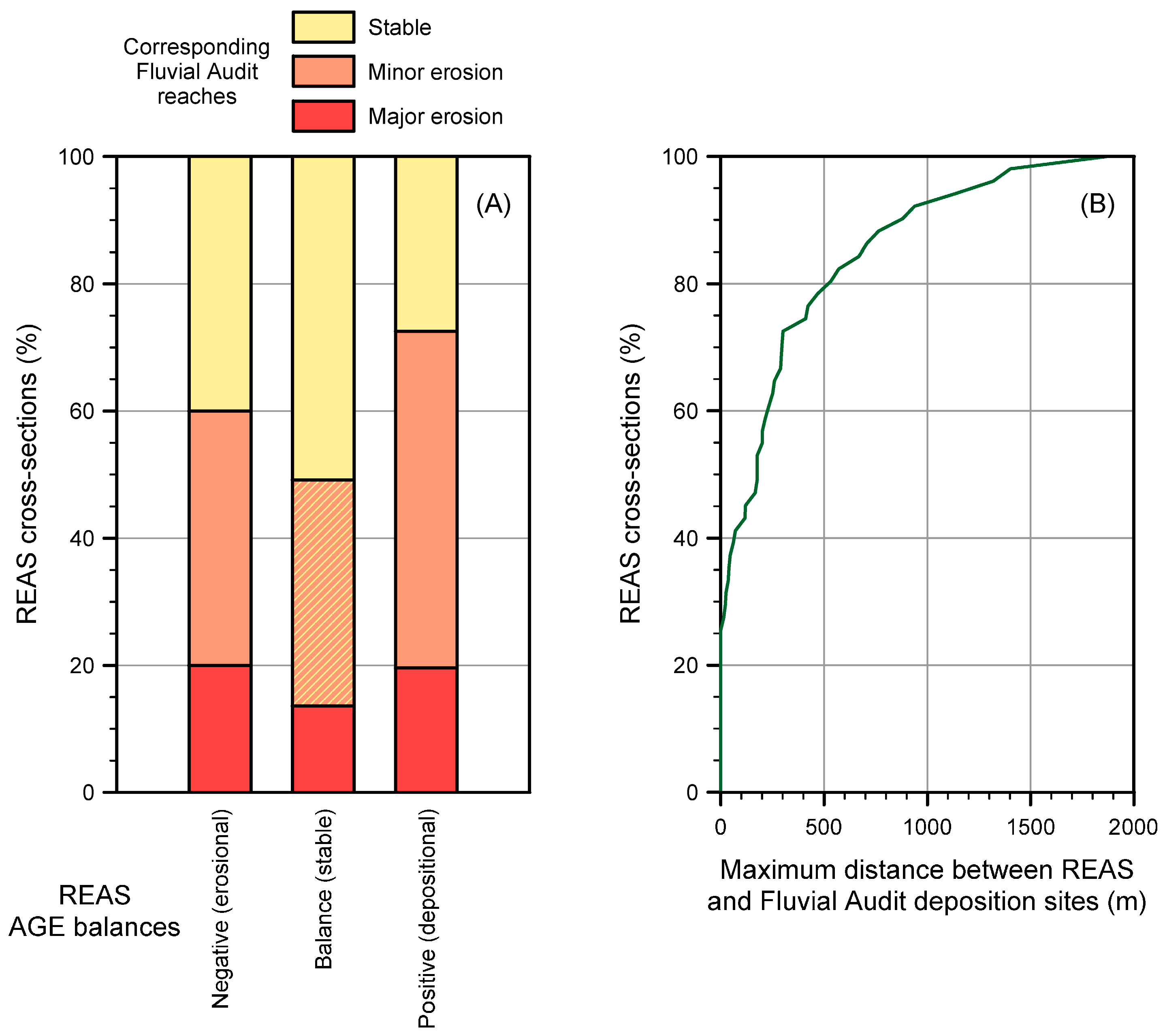
© 2017 by the authors. Licensee MDPI, Basel, Switzerland. This article is an open access article distributed under the terms and conditions of the Creative Commons Attribution (CC BY) license ( http://creativecommons.org/licenses/by/4.0/).
Share and Cite
MDPI and ACS Style
Soar, P.J.; Wallerstein, N.P.; Thorne, C.R. Quantifying River Channel Stability at the Basin Scale. Water 2017, 9, 133. https://doi.org/10.3390/w9020133
AMA Style
Soar PJ, Wallerstein NP, Thorne CR. Quantifying River Channel Stability at the Basin Scale. Water. 2017; 9(2):133. https://doi.org/10.3390/w9020133
Chicago/Turabian StyleSoar, Philip J., Nicholas P. Wallerstein, and Colin R. Thorne. 2017. "Quantifying River Channel Stability at the Basin Scale" Water 9, no. 2: 133. https://doi.org/10.3390/w9020133
Note that from the first issue of 2016, this journal uses article numbers instead of page numbers. See further details here.