Tracer Experiments and Hydraulic Performance Improvements in a Treatment Pond

Abstract

The treatment efficiency of a wetland constructed for nutrient removal depends strongly on the flow patterns and residence times of the wetland. In this study, a tracer experiment was performed to estimate the residence time distribution and the hydraulic efficiency of a treatment pond with shallow and deep-water areas. Rhodamine WT experiments revealed a non-uniform flow pattern in the deep-water area and an overall poor hydraulic efficiency in the wetland. To improve flow uniformity and hydraulic efficiency, several design options for different inlet–outlet configurations, flow rates, water depths, and emergent baffle additions were considered. The effects on hydraulic performance were investigated through mathematical model simulations. The results revealed that increasing the flow rate and decreasing the water depth slightly improved the hydraulic performance, whereas changing the positions of the inlet and outlet produced inconsistent effects. The most effective improvement involved installing emergent baffles, with the number of baffles presenting the largest positive effect, followed by the width and length of the baffles. Long and thin baffles resulted in a uniform flow velocity field, a meandering flow path, and greater residence times and effective volume ratios. The installation of two baffles increased the hydraulic efficiency to 1.00, indicating excellent hydraulic performance. The thin baffles occupied approximately 3.7%–6.3% of the deep-water area and 1.9%–3.2% of the entire pond, indicating the potential for their practical application in limited land use regions.

1. Introduction

Wetlands are highly beneficial, and promote biodiversity by providing habitats for plants, birds, and insects that have an affinity for aqueous environments. Treatment ponds are one type of artificial wetlands designed to provide multiple functions [1,2,3,4,5]. Such ponds are widely used in urban areas for storm water management, ecological conservation, and pollution treatment [6]. Degradation by microorganisms and adsorption by plants are two of the primary mechanisms for pollutant removal and degradation [7]. The overall effectiveness of both mechanisms is dependent on the residence time, or the length of time that water and pollutants are retained in the wetland. The treatment potential and efficiency of wetlands are usually related to the residence time of individual parcels of water within the wetland [8]. Wang and Mitsch [9] suggested that treatment could be improved by manipulating the hydraulic regime to improve hydraulic performance. Parameters such as the aspect ratio, bottom topography, water depth, vegetation, baffles, and inlet/outlet position can influence wetland hydrodynamics and determine both the retention time and hydraulic efficiency [10,11,12,13]. It has been suggested that hydraulic performance could be improved by allowing the flow to pass uniformly through the wetland and avoiding short-circuiting flows and dead zones [14].

Williams et al. [15] showed that ponds are the largest contributors to biodiversity, and supported more unique species than other types of waterbodies, such as rivers, streams, and ditches, in an agricultural landscape in southern England. A number of additional studies have confirmed this finding [16,17,18]. The hydraulics of ponds and wetlands can generally be evaluated through mathematical modeling [19,20] and tracer experiments [21,22]. This study investigated the flow hydrodynamics, residence time distribution, and hydraulic performance of a treatment pond using tracer experiments and mathematical modeling. A well-trained horizontal two-dimensional model was employed to simulate flow conditions and tracer concentrations in several scenarios involving 10 sets of flow rates, nine sets of water depths, nine sets of inlet and outlet locations, 14 sets of single emergent baffles, and six sets of two emergent baffles.

2. Methods

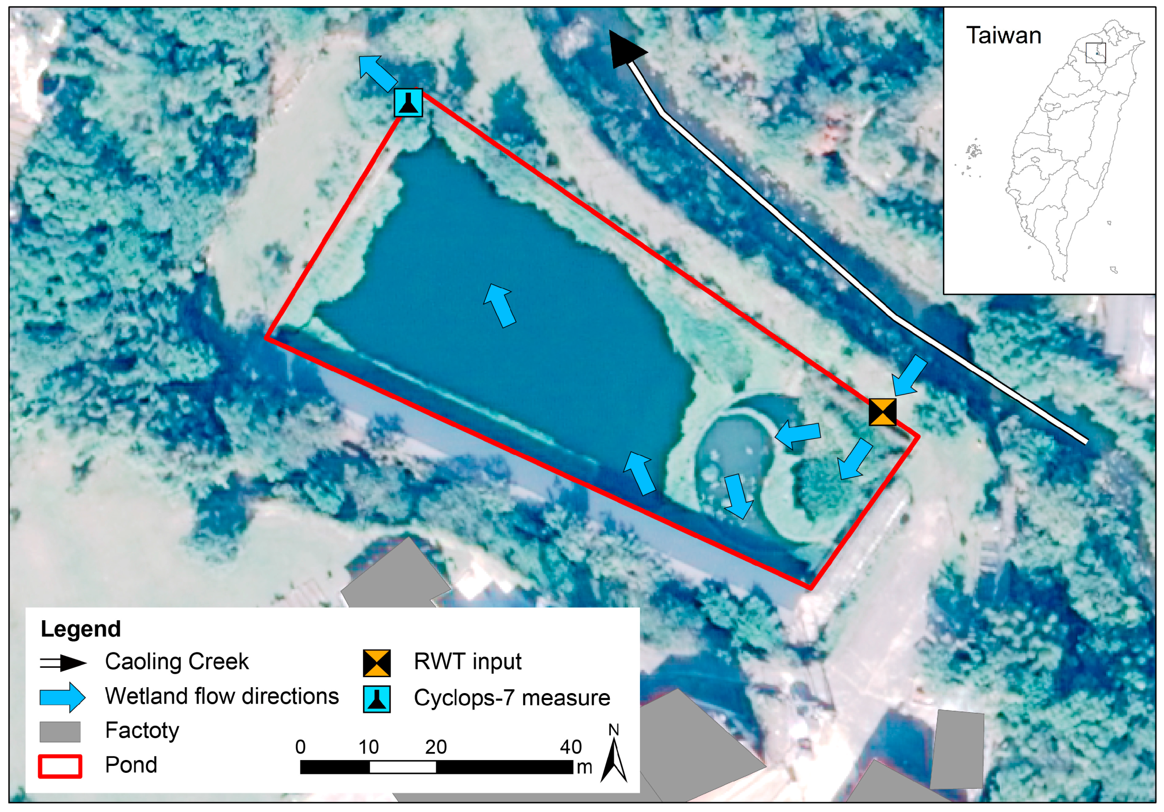
2.1. Study Area

Approximately 10,000 agricultural ponds were present 100 years ago on the Taoyuan Plateau, northern Taiwan. Historically, farmers used these ponds to preserve water for rice paddy irrigation. Thus, agricultural ponds were distributed throughout the plateau and connected by irrigation ditches to form artificial, but semi-natural, bird habitats [18]. The pond studied in this study is an agricultural pond located in Taoyuan County, northern Taiwan, on private land belonging to a soybean processing company (Figure 1). The factory produces large quantities of nutrient-rich wastewater that could cause pollution and damage the environment if directly discharged into the creek. To prevent this discharge, the factory installed a treatment pond to treat the turbid and odorous soybean wastewater. This pond was originally a swimming pool, but was abandoned. The authors incorporated the pool into a treatment wetland pond to treat soybean wastewater. Previous published studies [23,24,25], on the wetland include architectural design concepts, field observations, and experiments. The pond was designed with a hydraulic retention time (HRT) between 28 days and 30 days. Most of the substrate in the pond was embedded concrete elements below ground. Thus, porosity could be neglected in subsurface flow although the soil bank may facilitate lateral exchange with groundwater. The upstream section of the pond was designed to hold shallow water with a meandering flow. The downstream section is a large area of deeper, open water, and it has been suggested that the hydraulic performance of this deeper section could be improved. The water depth of the upstream section is approximately 1.0 m, and that of the downstream section is approximately 2.3 m. The length and width of the wetland are approximately 100 m and 35 m, respectively. In addition to the wastewater from the factory, the wetland receives clean water from Caoling Creek. The water and pollutants enter the wetland in the shallow-water area and exit from the deep-water area via a rectangular weir, which is designed to control the water depth of the wetland.

2.2. Tracer Experiments

Tracers are used in a variety of environments, such as those involving aquifers, streams, rivers, estuaries, reservoirs, lakes, and wetlands [26]. Rhodamine WT, a fluorescent xanthene dye, has long been used as a hydrologic tracer in surface water systems [27], including rivers and wetlands [28]. Dierberg and DeBusk [26] compared the applicability of rhodamine WT and lithium chloride as tracers in wetlands. Rhodamine WT has a recovery rate between 64% and 75%. As long as a complete concentration-time hydrograph can be obtained, an integral method can be used to analyze the residence time distribution (RTD) curve and calculate hydraulic parameters. Rhodamine WT meets regulations and is easily detectable with a portable fluorescence detector at concentrations as low as 0.01 μg·L⁻¹ [27,29,30,31]. Therefore, rhodamine WT was used as a tracer in the present study to observe the flow and diffusion of contaminants in the water body. A 200 mL volume of the tracer with a concentration of 25,000 mg·L⁻¹ was instantaneously added at the pond inlet. At the outlet, variations in the tracer concentration were measured over time to obtain the tracer response curve and the RTD curve and to assess the overall hydraulic performance of the wetland. In addition, a rectangular weir was installed at the outlet to measure the flow rate. A submerged underwater fluorescence meter (Cyclops-7, Turner Designs, San Jose, CA, USA) and an automatic recorder were installed in front of this weir to record changes in the tracer concentration every 30 min. Three different sets of experiments were conducted to assess three different flow rates (0.0026, 0.0011, and 0.0039 m³·s⁻¹) at the same water depth (2.0 m).

2.3. Hydraulic Performance

To assess the treatment efficiency and hydraulic performance of the wetlands, Persson et al. [11] presented a hydraulic efficiency equation:

$$\lambda =e_v\left(1-\frac{1}{N}\right)$$

(1)

where e_v is the effective volume ratio and N is the number of continuously stirred tank reactors (CSTR) in series. The hydraulic efficiency $\lambda$ can be categorized into three levels: (1) good hydraulic efficiency, $\lambda \ge 0.75$; (2) satisfactory hydraulic efficiency, $0.5<\lambda <0.75$; and (3) poor hydraulic efficiency, $\lambda \le 0.5$.

According to Thackston et al. [10], e_v indicates the utilization of the effective volume ratio of a detention system:

$$e_v=\frac{t_m}{t_n}$$

(2)

where t_n is the mean residence time in [h], as shown in Equation (3), and t_m is the nominal retention time in [h] calculated from the first moment of the tracer response curve [6]:

$$t_n=\frac{V}{Q}$$

(3)

where V is the volume of the pond in [m³] and Q is the flow rate in [m³·s⁻¹].

$$t_m=\frac{{{\displaystyle \int }}_0^{\infty }t\mathrm{cdt}}{{{\displaystyle \int }}_0^{\infty }\mathrm{cdt}}\approx \frac{{{\displaystyle \sum }}_{i=2}^n\left(\frac{t_i\mathrm{c}\left(t_i\right)+t_{i-1}\mathrm{c}\left(t_{i-1}\right)}{2}\right)\left(t_i-t_{i-1}\right)}{{{\displaystyle \sum }}_{i=2}^n\left(\frac{\mathrm{c}\left(t_i\right)+\mathrm{c}\left(t_{i-1}\right)}{2}\right)\left(t_i-t_{i-1}\right)}$$

(4)

where c is the tracer concentration in [μg·L⁻¹], t is the time of measurement [h], and t_m is the mean residence time in [h].

Kadlec and Knight [32] suggested an alternative formula for calculating N based on differences in the time of the peak outflow concentration and the nominal retention time:

$$N=\frac{t_n}{t_n-t_p}$$

(5)

where t_p is the time of the peak concentration in the tracer response curve measured at the outlet of the pond in [h].

Chang et al. [14] substituted Equations (2) and (5) into Equation (1) to obtain the hydraulic efficiency formula (Equation (6)), which is used to estimate the hydraulic efficiency in the present study:

$$\lambda =\frac{t_m\times t_p}{t_n^2}$$

(6)

2.4. Mathematical Model

To determine the spatial distribution of the flow and the tracer concentrations of the free-water area of the wetland, a horizontal two-dimensional hydrodynamic and water quality transport model (TABS-2) was developed. TABS-2 consists of two modules: RMA2 and RMA4. RMA2 and RMA4 were implemented for water velocity and tracer concentration calculations.

2.4.1. RMA2 Module

RMA2 is a two-dimensional depth-averaged finite element hydrodynamic model for computing the water surface elevations and horizontal velocity components of the subcritical free-surface flow field [33]. The governing equations of RMA2 pertain to mass and momentum conservation, as shown in Equations (7)–(9):

$$\frac{\partial h}{\partial t}+\frac{\partial \left(hu\right)}{\partial x}+\frac{\partial \left(hv\right)}{\partial y}=0$$

(7)

$$h\frac{\partial u}{\partial t}+hu\frac{\partial u}{\partial x}+hv\frac{\partial u}{\partial y}-\frac{h}{\rho }\left(E_{xx}\frac{{\partial }^{2}u}{\partial x^2}+E_{xy}\frac{{\partial }^{2}u}{\partial y^2}\right)+gh\left(\frac{\partial a}{\partial x}+\frac{\partial h}{\partial x}\right)+h{\tau }_x=0$$

(8)

$$h\frac{\partial v}{\partial t}+hu\frac{\partial v}{\partial x}+hv\frac{\partial v}{\partial y}-\frac{h}{\rho }\left(E_{yx}\frac{{\partial }^{2}v}{\partial x^2}+E_{yy}\frac{{\partial }^{2}v}{\partial y^2}\right)+gh\left(\frac{\partial a}{\partial y}+\frac{\partial h}{\partial y}\right)+h{\tau }_y=0$$

(9)

where x and y are the Cartesian coordinates of the horizontal and longitudinal directions, respectively, in [m]; t is time in [s]; ρ is the water density in [kg·m⁻³]; h is the water depth in [m]; u and v are the velocities in the x- and y-directions, respectively, in [m·s⁻¹]; E_xx, E_yy, E_xy and E_yx are the eddy viscosity coefficientsin [Pascal·s]; a is the elevation of the bottom in [m]; and τ_x and τ_y are external forces in the x- and y-directions, respectively, in [m·s⁻²].

2.4.2. RMA4 Module

RMA4 is a finite element water quality transport model in which the depth concentration distribution is assumed to be uniform [34], and its governing equation is given by Equation (10):

$$h\left(\frac{\partial c}{\partial t}+u\frac{\partial c}{\partial x}+v\frac{\partial c}{\partial y}-\frac{\partial }{\partial x}{D}_x\frac{\partial c}{\partial y}-\frac{\partial }{\partial y}{D}_y\frac{\partial }{\partial y}-\sigma +k_c+\frac{R\left(c\right)}{h}\right)=0$$

(10)

where c is the tracer concentration in [μg·L⁻¹], D_x and D_y are turbulent mixing (dispersion) coefficients in [m²·s⁻¹], σ is the source/sink of the constituent in [μg·L⁻¹·s⁻¹], k_c is the first-order decay coefficient of the tracer in [day⁻¹], and R(c) is the rainfall/evaporation rate. The first-order decay coefficient, k_c, was used in the model to simulate the non-conservative behavior of rhodamine WT [35,36,37].

2.4.3. Determination of Parameters

There are five parameters that must be determined in TABS-2: (1) the roughness value, n, which was estimated from an empirical formula and set as 0.035–0.045 due to different vegetation; (2) the temperature, T, which was obtained from field measurements and ranged from 24 to 35 °C; (3) the eddy viscosity, E, the dispersion coefficient, D, and the decay coefficient, k_c, which were determined via the parameter calibration and model verification process described in Section 3.2.1.

2.4.4. Determination of Boundary Conditions

The TABS-2 model was developed based on field surveys, including surveys of the pond topography, flow rate, water surface elevation, and tracer concentrations. The topography of the pond was investigated using a TOPCON Total Station (GTS226, TOPCON, Tokyo, Japan) and was used to develop the fixed boundary of the RMA2 model. A rectangular weir was installed at the outlet to measure the flow rate using the weir formula. A HOBO Water Level Logger (model U20-001-01, Onset, Bourne, MA, USA) was installed in the deep-water area to record the water stage every 60 min. The investigated flow rates and water depths were entered as the upstream and the downstream boundaries of the RMA2 model. The pulse-input concentration of the tracer described was set as the upstream boundary of the RMA4 model, as discussed in Section 2.2.

2.4.5. Numerical Experiments

After parameter calibration and model verification, several numerical experiments were proposed and conducted. The effects of decreased water depth, increased flow rate, and installed baffles in the deep-water area and alterations at the locations of the inlet and outlet were evaluated. Ten cases of different flow rates and nine cases of different water depths were investigated. The water depth was the same (2.0 m) in cases of different flow rates. Additionally, the flow rate was also the same (0.002 m³·s⁻¹) in cases of different water depths. Nine cases of different inlet and outlet locations were also investigated. The following inlets and outlets were tested: Case IO-0 was the original site design (i.e., inlet and outlet located at the corners); in Case IO-1, the inlet was located at the corner and the outlet at the boundary midpoint; and in Case IO-2, the inlet was located at the corner and the outlet on the diagonal. The flow rate and water depth for the cases of different inlet and outlet locations were set to constant values of 0.002 m³·s⁻¹ and 2.0 m, respectively.

In addition, Shih et al. [6] and Chang et al. [14] suggested that the addition of emergent baffles could considerably alter the hydraulic efficiency in a deep-water wetland. Therefore, several baffles with different lengths, widths, and aspect ratios were modeled. The aspect ratio is calculated as the baffle length divided by the baffle width, whereas the length and width are defined as the distances parallel and perpendicular to the flow direction. Fourteen cases of placing a single baffle and six cases of placing two baffles were investigated. The flow rate and water depth for these cases were set to constant values of 0.002 m³·s⁻¹ and 2.0 m, respectively.

3. Results and Discussion

3.1. Tracer Experiments

Three tracer conductance experiments were performed. Peak values of different concentrations were observed, and the findings were consistent to those of Bodin et al. [38]. In the first experiment, the highest peak tracer concentration (11.9 μg·L⁻¹) occurred at t = 76.5 h after introduction of the tracer. A second peak appeared at t = 100.0 h. Approximately 10 days after the beginning of the experiment, the tracer concentration returned to the baseline level (Figure 2a). In the second experiment, the peak value of 7.85 μg·L⁻¹ was measured at t = 98.0 h. On approximately the 11th day, the values returned to the baseline (Figure 2b). In the third experiment, a peak value of 10.0 μg·L⁻¹ was measured at t = 75.0 h. On approximately the 8th day, the values returned to the baseline (Figure 2c). The effective volume ratios were estimated as 0.56 in Experiment No. 1 (Exp. 1), 0.25 in Exp. 2, and 0.26 in Exp. 3. The hydraulic efficiencies were calculated as 0.18 in Exp. 1, 0.02 in Exp. 2, and 0.05 in Exp. 3 (

Table 1. Model validation by field measurements of hydraulic retention time, effective volume ratio, and hydraulic efficiency.

Experiment		tn (h)	tm (h)	tp (h)	ev	λ
1	Field	239.6	134.2	76.5	0.56	0.18
	Model	239.6	135.8	66.5	0.57	0.16
2	Field	860.3	169.4	98.0	0.25	0.02
	Model	860.3	211.6	90.0	0.25	0.03
3	Field	354.8	90.6	75.0	0.26	0.05
	Model	354.8	135.1	68.5	0.38	0.07

). The pond exhibited a generally poor hydraulic performance. The experiments yielded a complete concentration hydrograph and, because rainfall did not occur during the survey, these data were used to adjust the parameters of the mathematical model.

3.2. Mathematical Model Simulation

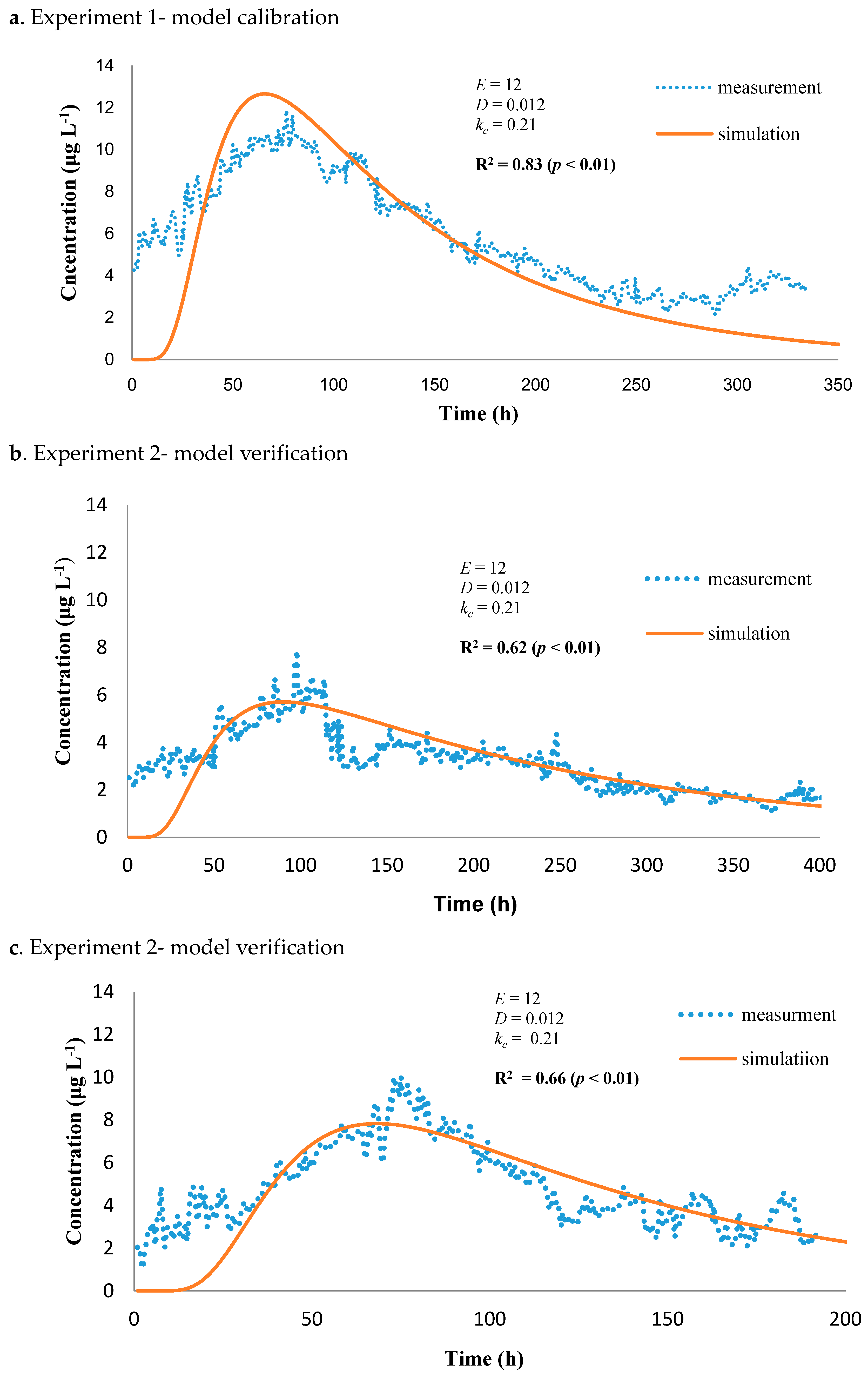
3.2.1. Parameter Calibration and Model Verification

The model simulations were compared to field observations of the tracer response curves (Figure 2). Parameters such as the eddy viscosity (E), dispersion coefficient (D), and decay coefficient (k_c) were adjusted from experiment 1 (calibration) and determined from experiments 2 and 3 (verification). The correlation coefficients (R²) between field investigations and model simulations were 0.83, 0.62, and 0.66, and they indicated significant dependence between the measured and simulated results (p < 0.01). The simulated and measured tracer concentration values were consistent, except for the background concentrations and tracer tails of all of the experiments and the peak concentrations of experiments 2 and 3. The invalid tracer tails were due to transient storage, which was attributable to hyporheic exchange [28]. Although most areas of pond bed were embedded with concrete, other areas such as the pond bank exhibited possible signs of lateral hyporheic exchange through the bank (S.S. Shih, personal observations). Although the model simulations did not yield background and peak concentrations that were consistent with field observations, the key hydraulic parameters derived from the method of moments were not affected [26], suggesting comparable values of effective volume ratio and hydraulic efficiency (Table 1). The results indicated that the mathematical model simulations yielded acceptable calculations of hydraulic performance.

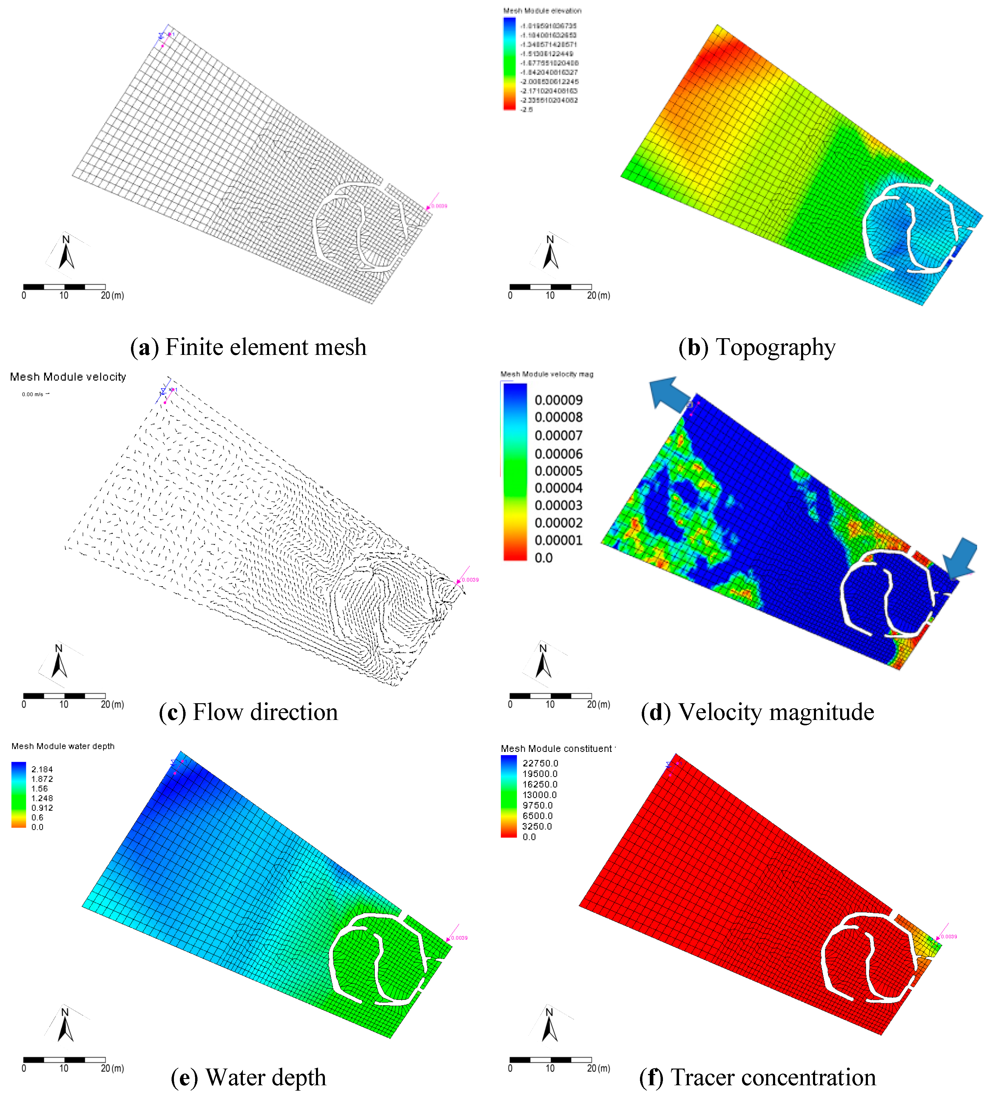
3.2.2. Flow Hydrodynamics and Hydraulic Performance

The observed two-dimensional horizontal distributions of the flow direction, flow velocity, and tracer concentrations are illustrated in Figure 3. The spatial distribution of the flow velocity was non-uniform and consistent with the results of previous tracer experiments [39]. The flow velocity ranged from 0.00005 m·s⁻¹ to 0.0001 m·s⁻¹ in the shallow-water area and from 0.00001 m·s⁻¹ to 0.00008 m·s⁻¹ in the deep-water area. The water depth ranged from 0.8 m to 1.2 m in the shallow-water area and from 1.2 m to 2.5 m in the deep-water area. The Froude number ranged from 0.32 to 0.56 in the shallow-water area and from 0.12 to 0.39 in the deep-water area, which indicated a subcritical flow condition in the entire pond. The results indicated a low velocity, deeper water, and non-uniform flow conditions in the deep-water area relative to those in the shallow-water area. The dead zones (i.e., areas with a flow velocity below 0.00005 m·s⁻¹) occurred in the upper right corner and lower left corner of the deep-water area, which may have decreased the hydraulic performance by inhibiting water exchange with other zones. A region of short-circuited flow (i.e., a region of high flow velocity) was observed from the lower right corner to the upper left corner of the deep-water area, which may have reduced the residence time and flow uniformity and thereby decreased the hydraulic performance and treatment efficiency. The poor hydraulic efficiency resulted primarily from short-circuited flow and the presence of a dead zone in the deep-water area. Hydraulically, treatment efficiency is considered satisfactory as long as the system is well mixed and the physical characteristics are uniform across the wetland perpendicular to the flow [40]. The poor treatment efficiencies of suspended solids were detected due to the occurrence of short-circuited flow. In addition, a low nitrogen removal rate was likely due to the dead zone in the deep-water area. The results may be different for other pollutants, such as biochemical oxygen demand (BOD), for which adsorption does not occur.

3.3. Changing the Flow Rate and Water Depth to Improve Hydraulic Performance

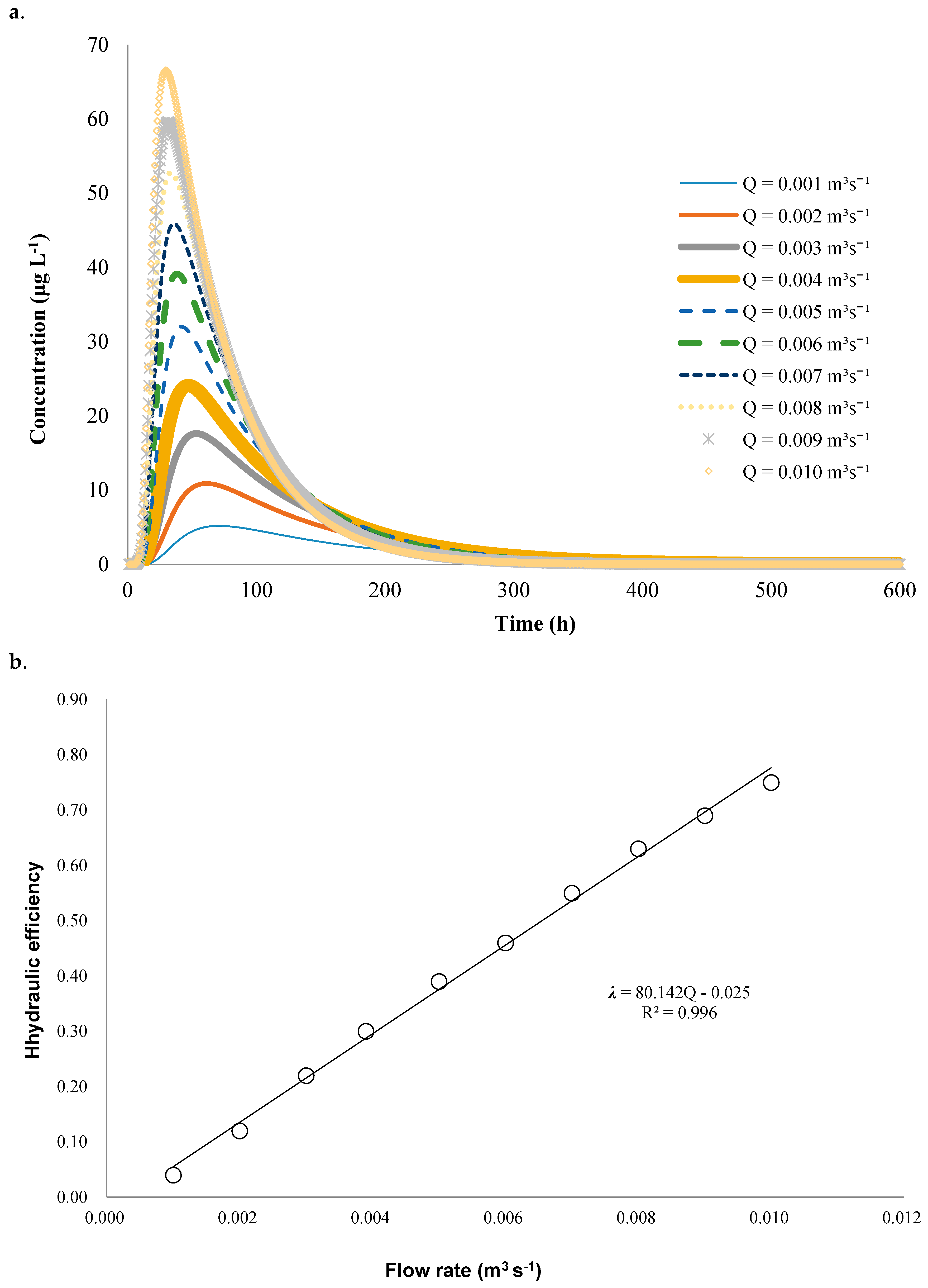
3.3.1. Flow Rate

Ten cases of different flow rates were investigated. The flow velocity and flow uniformity increased with increasing flow rate. Based on the tracer response curves and RTD curve analysis, increasing the flow rate (from 0.001 m³·s⁻¹ to 0.010 m³·s⁻¹) decreased the nominal retention time (t_n), mean residence time (t_m) and time of peak concentration (t_p) values. The effective volume ratio and the hydraulic efficiency increased with increasing flow rate. The increase in the flow rate exhibited a positive linear relationship with the hydraulic efficiency (Figure 4). When the flow rate was increased to 0.010 m³·s⁻¹, the hydraulic efficiency increased to a satisfactory level (λ = 0.74).

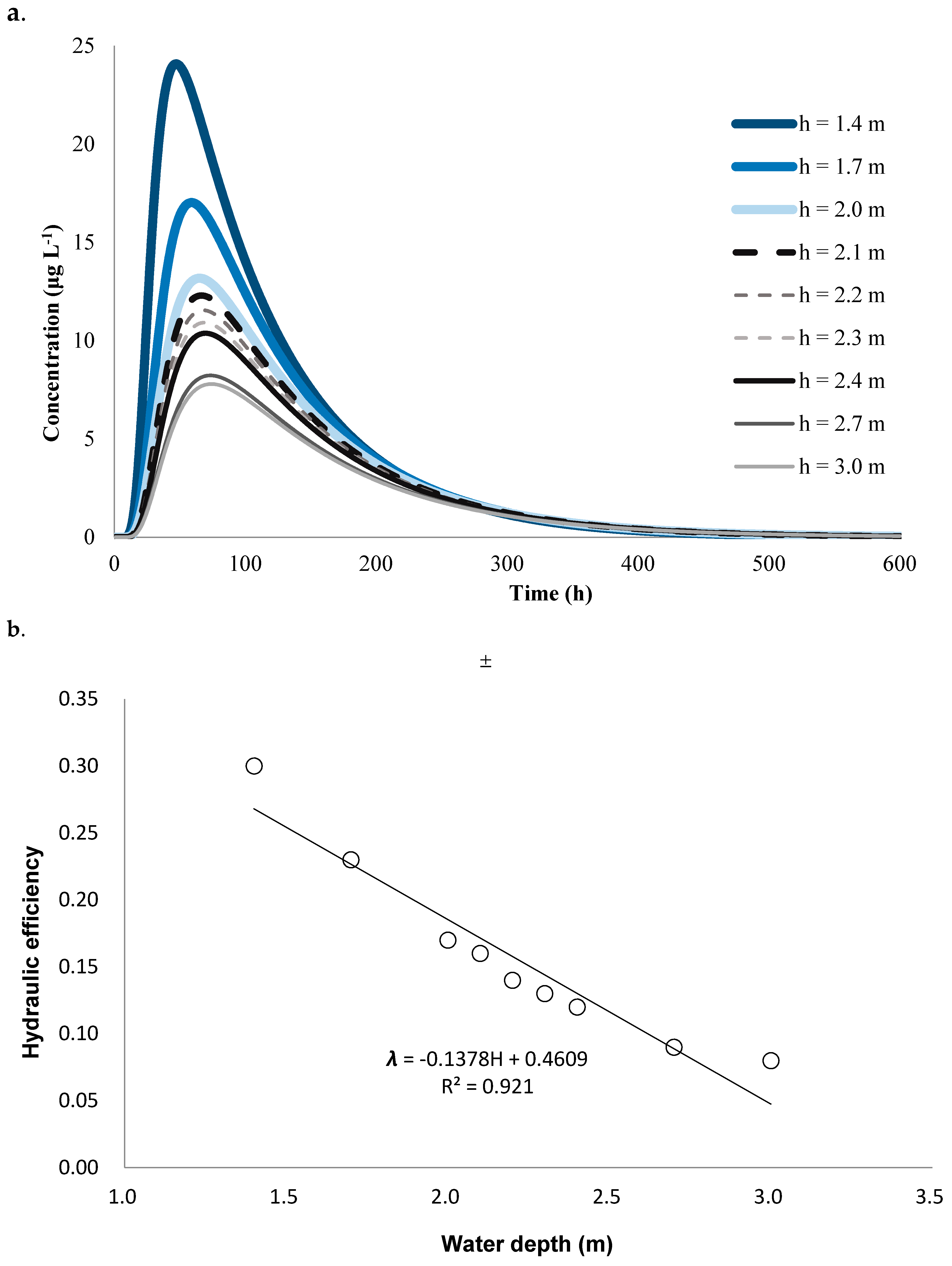
3.3.2. Water Depth

Nine cases of different water depths were investigated. The flow velocity and flow uniformity increased with decreasing water depth. At shallower water depths, the difference between the mean residence time (t_m) and the nominal retention time (t_n) was reduced, which increased the effective volume ratio. In addition, at greater water depths, longer mean residence time (t_m) values and lower effective volume ratios were observed, which resulted in a reduction in hydraulic efficiency. Water depth exhibited a negative linear relationship with hydraulic efficiency (Figure 5). By decreasing the water depth of the pond outlet to 1.4 m, the hydraulic efficiency was increased to 0.30, which indicated a poor hydraulic level. Decreasing the downstream water depth yielded slight improvements in the effective volume ratio and hydraulic efficiency.

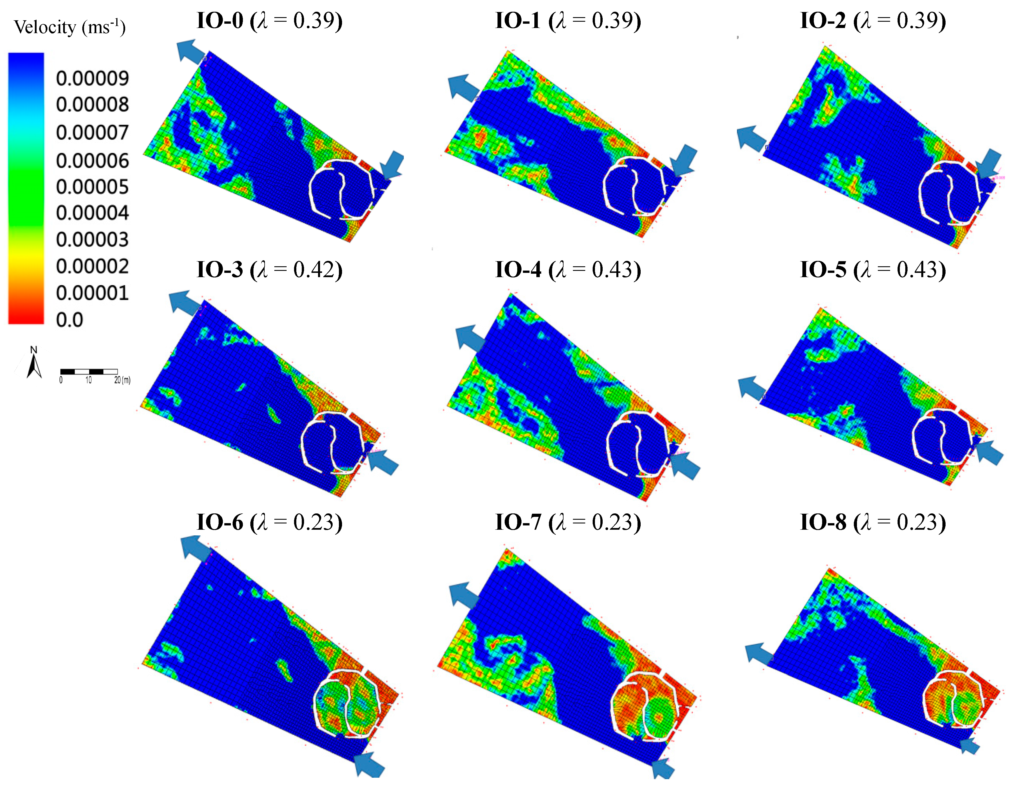
3.4. Altering Inlet and Outlet Locations to Improve Hydraulic Performance

Nine sets of different inlet and outlet locations were investigated. The results indicated that changing the location of the outlet did not significantly improve flow uniformity or the hydraulic efficiency (Figure 6). When moving the inlet from the upper right corner to the midpoint (Cases IO-3 to IO-5), the hydraulic efficiency slightly increased. By contrast, when the inlet was moved from the upper right corner to the lower right corner (Cases IO-6 to IO-8), the hydraulic efficiency was reduced. Changing the inlet and outlet positions yielded inconsistent effects on the hydraulic efficiency.

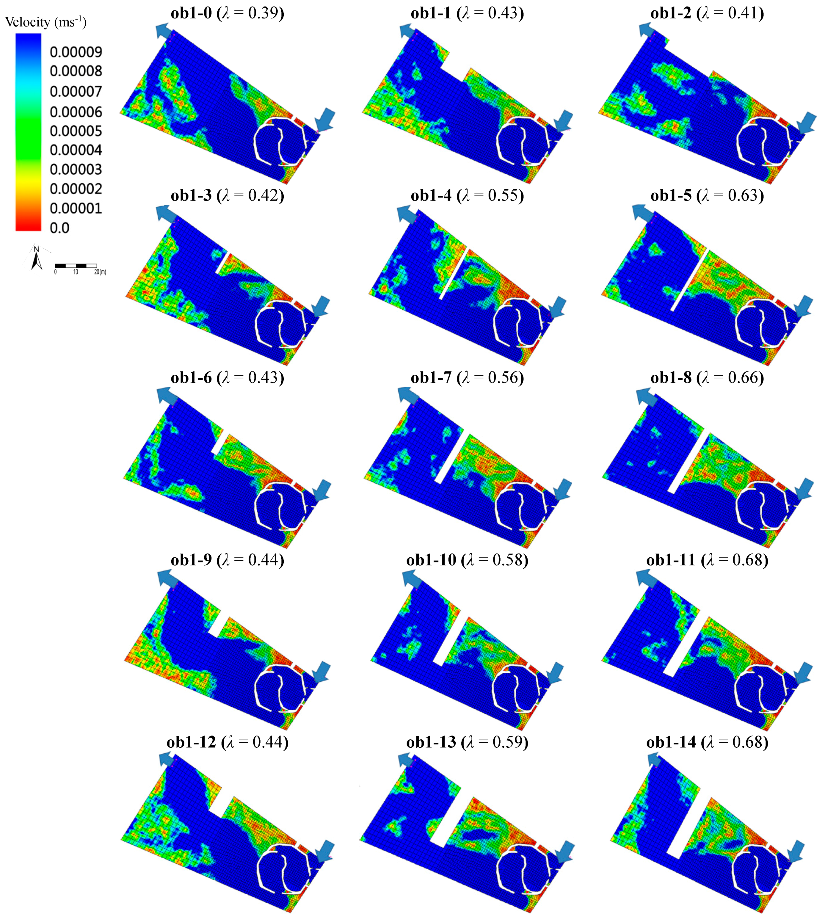
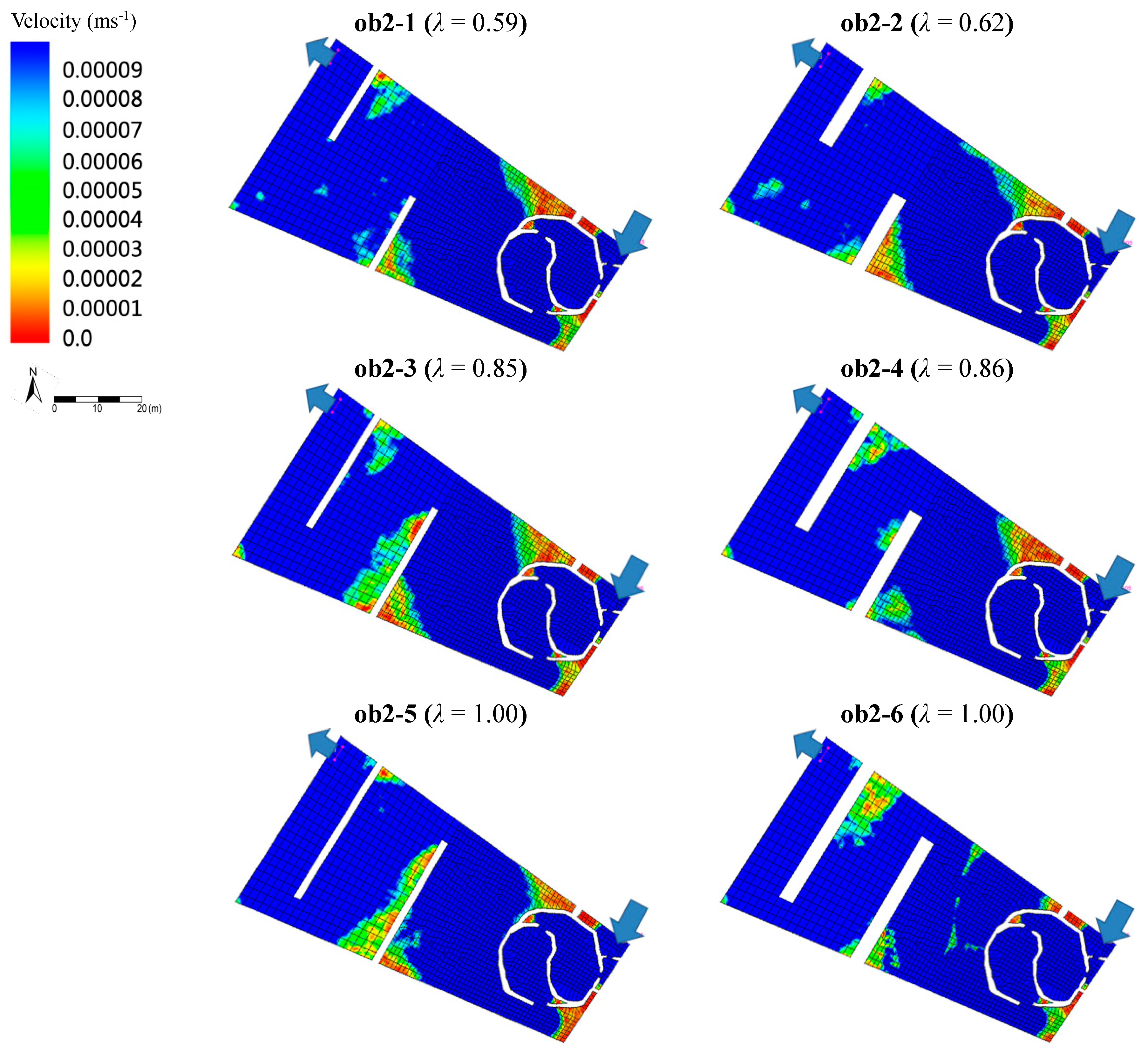
3.5. Adding Emergent Baffles to Improve Hydraulic Performance

This hypothesis considered determining whether poor hydraulic performance was related to the low removal rate of pollutants in deep-water areas of the downstream section of the pond. Fourteen different placements of a single emergent baffle were investigated. The baffles were placed in the same locations in the deep-water area. The results of flow field simulations are shown in Figure 7. Case ob1-0 represents the current conditions, and the other cases represent the experimental scenarios. When the baffle width was 35.8 m, the hydraulic efficiency increased to 0.63 (Case ob1-5), whereas increasing the length did not produce significant improvements (Case ob1-11 and Case ob1-14). The width of the baffle was found to be crucial for improving the hydraulic efficiency. The best hydraulic efficiency of 0.68 was achieved by adding a single baffle. The placement of two emergent baffles was also considered, for which six cases were investigated (Figure 8). Cases ob2-5 and ob2-6 performed the best, followed by cases ob2-3 and ob2-4. Cases ob2-1 and ob2-2 had the worst performance. The placement of two baffles positively increased the hydraulic efficiency to 1.00 because it caused the waterway in the deep-water region to meander and effectively reduced the dead zone area and short-circuited flow. In the case of short-circuiting flow within a wetland, both the residence time and the volume of the wetland through which the water travels were reduced [40]. In heterogeneous wetlands, specifically wetlands with substantial variations in water depth, vegetation, and other physical characteristics, the physical, chemical, and biological processes will affect the quality of the water differently compared to homogenous wetlands, in which there is little variation in biotic and physical characteristics. In addition, the baffles occupied approximately 3.7%–6.3% of the deep-water area and 1.9%–3.2% of the entire wetland, indicating the potential for their practical application in limited land use regions.

4. Conclusions

This study presents a field investigation of the RTD and hydraulic efficiency in a treatment pond using tracer experiments and mathematical model simulations. Preferential flow and dead zones were found to occur in the deep-water area of the wetland, and produced a non-uniform velocity field and poor hydraulic performance. Methods of improving the hydraulic efficiency of the deep-water area, including manipulating nine sets of water depths, 10 sets of flow rates, 14 sets of adding single emergent baffles, and six sets of adding two emergent baffles, were investigated and evaluated. Changing the positions of the inlet and outlet had minimal effects, whereas increasing the flow rate and decreasing the water depth slightly increased the flow uniformity and hydraulic efficiency. Installing emergent baffles had the most obvious effects, with these baffles resulting in meandering flow paths, prevention of short-circuiting flows, and enhancement of the hydraulic efficiency. Long and thin baffles caused obvious meandering flow paths with higher residence times, and after installing one or two thin baffles, hydraulic efficiency was improved. The main conclusion is that channeling was caused by the short-circuited flow. This result suggests that installing baffles could dramatically improve the poor hydraulic performance in the deep-water area of the wetland.

References

- Zedler, J.B.; Kercher, S. Wetland resources: Status, trends, ecosystem services, and restorability. Annu. Rev. Environ. Resour. 2005, 30, 39–74. [Google Scholar] [CrossRef]
- Tranvik, L.J.; Downing, J.A.; Cotner, J.B.; Loiselle, S.A.; Striegl, R.G.; Ballatore, T.J.; Dillon, P.; Finlay, K.; Fortino, K.; Knoll, L.B.; et al. Lakes and reservoirs as regulators of carbon cycling and climate. Limnol. Oceanogr. 2009, 54, 2298–2314. [Google Scholar] [CrossRef]
- Hsu, C.; Hsieh, H.; Yang, L.; Wu, S.; Chang, J.; Hsiao, S.; Su, H.; Yeh, C.; Ho, Y.; Lin, H. Biodiversity of constructed wetlands for wastewater treatment. Ecol. Eng. 2011, 37, 1533–1545. [Google Scholar] [CrossRef]
- Virginia Department of Transportation. BMP Design Manual of Practice; Virginia Department of Transportation: Springfield, VA, USA, 2013. [Google Scholar]
- Yam, R.; Hsu, C.; Chang, T.; Chang, W. A preliminary investigation of wastewater treatment efficiency and economic cost of subsurface flow oyster-shell-bedded constructed wetland systems. Water 2013, 5, 893–916. [Google Scholar] [CrossRef]
- Shih, S.-S.; Hong, S.-S.; Chang, T.-J. Flume experiments for optimizing the hydraulic performance of a deep-water wetland utilizing emergent vegetation and obstructions. Water 2016, 8, 265. [Google Scholar] [CrossRef]
- Toet, S.; Van Logtestijn, R.S.P.; Schreijer, M.; Kampf, R.; Verhoeven, J.T.A. The functioning of a wetland system used for polishing effluent from a sewage treatment plant. Ecol. Eng. 2005, 25, 101–124. [Google Scholar] [CrossRef]
- Wahl, M.D.; Brown, L.C.; Soboyejo, A.O.; Dong, B. Quantifying the hydraulic performance of treatment wetlands using reliability functions. Ecol. Eng. 2012, 47, 120–125. [Google Scholar] [CrossRef]
- Wang, N.; Mitsch, W.J. A detailed ecosystem model of phosphorus dynamics in created riparian wetlands. Ecol. Model. 2000, 126, 101–130. [Google Scholar] [CrossRef]
- Thackston, E.L.; Shields, F.D.; Schroeder, P.R. Residence time distributions of shallow basins. J. Environ. Eng. 1987, 113, 1319–1332. [Google Scholar] [CrossRef]
- Persson, J.; Somes, N.; Wong, T. Hydraulics efficiency of constructed wetlands and ponds. Water Sci. Technol. 1999, 40, 291–300. [Google Scholar] [CrossRef]
- Su, T.-M.; Yang, S.-C.; Shih, S.-S.; Lee, H.-Y. Optimal design for hydraulic efficiency performance of free-water-surface constructed wetlands. Ecol. Eng. 2009, 35, 1200–1207. [Google Scholar] [CrossRef]
- Shih, S.-S.; Kuo, P.-H.; Fang, W.-T.; LePage, B.A. A correction coefficient for pollutant removal in free water surface wetlands using first-order modeling. Ecol. Eng. 2013, 61, 200–206. [Google Scholar] [CrossRef]
- Chang, T.; Chang, Y.; Lee, W.; Shih, S. Flow uniformity and hydraulic efficiency improvement of deep-water constructed wetlands. Ecol. Eng. 2016, 92, 28–36. [Google Scholar] [CrossRef]
- Williams, P.; Whitfield, M.; Biggs, J.; Bray, S.; Fox, G.; Nicolet, P.; Sear, D. Comparative biodiversity of rivers, streams, ditches and ponds in an agricultural landscape in southern England. Biol. Conserv. 2004, 115, 329–341. [Google Scholar] [CrossRef]
- Usseglio-Polatera, P. Theoretical habitat templets, species traits, and species richness: Aquatic insects in the upper Rhône River and its floodplain. Freshw. Biol. 1994, 31, 417–437. [Google Scholar] [CrossRef]
- Verdonschot, P.F.M. Integrated ecological assessment methods as a basis for sustainable catchment management. Hydrobiologia 2000, 422, 389–412. [Google Scholar] [CrossRef]
- Fang, W.-T.; Chu, H.-J.; Cheng, B.-Y. Modeling waterbird diversity in irrigation ponds of Taoyuan, Taiwan using an artificial neural network approach. Paddy Water Environ. 2009, 7, 209–216. [Google Scholar] [CrossRef]
- Min, J.; Wise, W.R. Simulating short-circuiting flow in a constructed wetland: The implications of bathymetry and vegetation effects. Hydrol. Process. 2009, 23, 830–841. [Google Scholar] [CrossRef]
- Wang, Y.; Song, X.; Liao, W.; Niu, R.; Wang, W.; Ding, Y.; Wang, Y.; Yan, D. Impacts of inlet–outlet configuration, flow rate and filter size on hydraulic behavior of quasi-2-dimensional horizontal constructed wetland: NaCl and dye tracer test. Ecol. Eng. 2014, 69, 177–185. [Google Scholar] [CrossRef]
- Headley, T.R.; Kadlec, R.H. Conducting hydraulic tracer studies of constructed wetlands: A practical guide. Ecohydrol. Hydrobiol. 2007, 7, 269–282. [Google Scholar] [CrossRef]
- Kadlec, R.H. Tracer and spike tests of constructed wetlands. Ecohydrol. Hydrobiol. 2007, 7, 283–295. [Google Scholar] [CrossRef]
- Huang, K.-H.; Fang, W.-T. Developing concentric logical concepts of environmental impact assessment systems: Feng Shui concerns and beyond. J. Archit. Plan. Res. 2013, 31, 39–55. [Google Scholar]
- Fang, W.-T.; Cheng, B.-Y.; Shih, S.-S.; Chou, J.-Y.; Otte, M.L. Modelling driving forces of avian diversity in a spatial configuration surrounded by farm ponds. Paddy Water Environ. 2016, 14, 185–197. [Google Scholar] [CrossRef]
- Fang, W.-T.; Chou, J.-Y.; Lu, S.-Y. Simple patchy-based simulators used to explore pondscape systematic dynamics. PLoS ONE 2014, 9, e86888. [Google Scholar] [CrossRef] [PubMed]
- Dierberg, F.E.; DeBusk, T.A. An evaluation of two tracers in surface-flow wetlands: Rhodamine-WT and lithium. Wetlands 2005, 25, 8–25. [Google Scholar] [CrossRef]
- Smart, P.L.; Laidlaw, I.M.S. An evaluation of some fluorescent dyes for water tracing. Water Resour. Res. 1977, 13, 15–33. [Google Scholar] [CrossRef]
- Runkel, R.L. On the use of rhodamine WT for the characterization of stream hydrodynamics and transient storage. Water Resour. Res. 2015, 51, 6125–6142. [Google Scholar] [CrossRef]
- Wilson, J.F., Jr. Techniques of Water-Resources Investigations of the United States Geological Survey; United States Geological Survey: Washington, DC, USA, 1968.
- Kilpatrick, F.A.; Wilson, J.F., Jr. Techniques of Water-Resources Investigations of the United States Geological Survey; United States Geological Survey: Denver, CO, USA, 1982.
- Lin, A.Y.; Debroux, J.; Cunningham, J.A.; Reinhard, M. Comparison of rhodamine WT and bromide in the determination of hydraulic characteristics of constructed wetlands. Ecol. Eng. 2003, 20, 75–88. [Google Scholar] [CrossRef]
- Kadlec, R.H.; Knight, R.L. Treatment Wetlands; CRC Press, Lewis Publishers: Boca Raton, FL, USA, 1996. [Google Scholar]
- Donnell, B.P.; Letter, J.V.; McAnally, W.H. Users Guide to RMA2; Version 4.5; U.S. Army, Engineer Research and Development Center: Vicksburg, MS, USA, 2009; pp. 3–5. [Google Scholar]
- Letter, J.V.; Donnell, B.P. Users Guide to RMA4; Version 4.5; U.S. Army, Engineer Research and Development Center: Vicksburg, MS, USA, 2008; pp. 2–4. [Google Scholar]
- Fernald, A.G.; Wigington, P.J., Jr.; Landers, D.H. Transient storage and hyporheic flow along the Willamette River, Oregon: Field measurements and model estimates. Water Resour. Res. 2001, 37, 1681–1694. [Google Scholar] [CrossRef]
- Laenen, A.; Bencala, K.E. Transient storage assessments of dye-tracer injections in rivers of the Willamette Basin, Oregon. J. Am. Water Resour. Assoc. 2001, 37, 367–377. [Google Scholar] [CrossRef]
- Writer, J.H.; Ryan, J.N.; Keefe, S.H.; Barber, L.B. Fate of 4-nNonylphenol and 17β-estradiol in the Redwood River of Minnesota. Environ. Sci. Technol. 2012, 46, 860–868. [Google Scholar] [CrossRef] [PubMed]
- Bodin, H.; Mietto, A.; Ehde, P.M.; Persson, J.; Weisner, S.E.B. Tracer behaviour and analysis of hydraulics in experimental free water surface wetlands. Ecol. Eng. 2012, 49, 201–211. [Google Scholar] [CrossRef]
- Kjellin, J.; Wörman, A.; Johansson, H.; Lindahl, A. Controlling factors for water residence time and flow patterns in Ekeby treatment wetland, Sweden. Adv. Water Resour. 2007, 30, 838–850. [Google Scholar] [CrossRef]
- Williams, C.F.; Nelson, S.D. Comparison of rhodamine-WT and bromide as a tracer for elucidating internal wetland flow dynamics. Ecol. Eng. 2011, 37, 1492–1498. [Google Scholar] [CrossRef]