Where to Find Water Pipes and Sewers?—On the Correlation of Infrastructure Networks in the Urban Environment

Abstract

Urban water infrastructure, i.e., water supply and sewer networks, are underground structures, implying that detailed information on their location and features is not directly accessible, frequently erroneous, or missing. For public use, data is also not made available due to security concerns. This lack of quality data, especially for research purposes, requires substantial effort when such data is sought for both statistical and model-based analyses. An alternative to gathering data from archives and observations is to extract the information from surrogate data sources (e.g., the street network). The key for such an undertaking is to identify the common characteristics of all urban infrastructure network types and to quantify them. In this work, the network correlations of the street, water supply, and sewer networks are systematically analyzed. The results showed a strong correlation between the street networks and urban water infrastructure networks, in general. For the investigated cases, on average, 50% of the street network length correlates with 80%–85% of the total water supply/sewer network. A correlation between street types and water infrastructure properties (e.g., pipe diameter) cannot be found. All analyses are quantified in the form of different geometric- and graph-based indicators. The obtained results improve the understanding of urban network infrastructure from an integrated point of view. Moreover, the method can be fundamental for different research purposes, such as data verification, data completion, or even the entire generation of feasible datasets.

1. Introduction

In an urban system, a substantial number of public infrastructures can be represented in the form of a network, e.g., streets, subway systems, water supply pipes, and sewer pipes. The fundamental work of Strogatz [1], on the dynamics of complex networks, and Milo, et al. [2], on the design of network systems by motifs, allows an understanding and utilization of the advantages of such a structured approach.

The application of complex network analysis procedures to urban street networks has been shown by several authors, e.g., Porta, et al. [3], Jiang and Claramunt [4] and Yin, et al. [5]. For sewer networks, Urich, et al. [6] suggested using a graph-theoretical approach, and Möderl, et al. [7] used graph theory to describe water supply networks. Additionally, Sitzenfrei, et al. [8] analyzed automatically generated water distribution system data based on GIS data. All of these investigations are specifically for one single network type.

One of the key issues of urban water infrastructure is that the pipes and sewers are underground structures with direct and obvious spatial information on the location only given at the manholes. The sheer size of the network (the typical dimension of the specific pipe length per person is 10 m) often results in unclear, wrong, and occasionally missing data. Hence, the required data for network analysis (likewise, statistical- and model-based) is often not completely available, not freely accessible (due to security concerns), or of poor quality (e.g., wrong data records of infrastructure element properties). Therefore, a substantial amount of time is spent in data collection and observation. However, even if data is available, it is frequently not stored in a digitized format needed for further processing (e.g., ESRI Shapefile). High-resolution spatial infrastructure data (e.g., consumption data at the household level) belong to different authorities, complicating the exchange and arbitrarily intersecting the data in terms of legal aspects even more (e.g., the exchange of data with third parties is often forbidden and subject to legal terms and conditions of operating companies). Thus, even though datasets exist, legal aspects may counteract a successful data exchange. Considering that the evolvement of water infrastructure networks began several decades ago [9], the availability of historical data is even worse. In this case, information on the build year of network components is indispensable. Finding alternative approaches to generate and extract missing data out of alternative data sources (surrogate data) on infrastructure networks is, therefore, a relevant research topic—notably for the purpose of model-building, especially for research purpose.

Blumensaat, et al. [10] reported an algorithm for creating hydrodynamic sewer models with limited data using street network data downloaded from OpenStreetMap as the input. This approach assumes a strong correlation between the street and sewer network (the authors estimate the spatial congruence to be between 30% and 95%). Following this idea, the question arises whether and how the street network data, which is easily accessible at a high quality, can assist in gaining knowledge of other urban infrastructure, such as water networks.

With an algorithm to complement the missing information on the urban water infrastructure based on available and easily accessible data (e.g., street data), the hydraulic behavior of the water supply and sewer networks could be assessed. Even when the entire water network information is missing, possible water networks can easily be created without a substantial effort, and these data can be used in further evaluations. Although the data will not be exact, it will resemble a possible network layout, allowing for a realistic modeling endeavor in the scientific context.

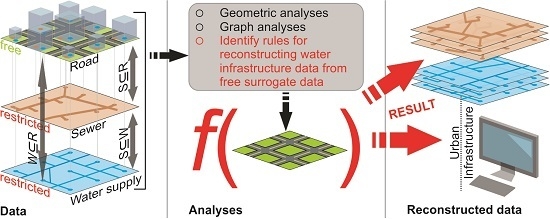
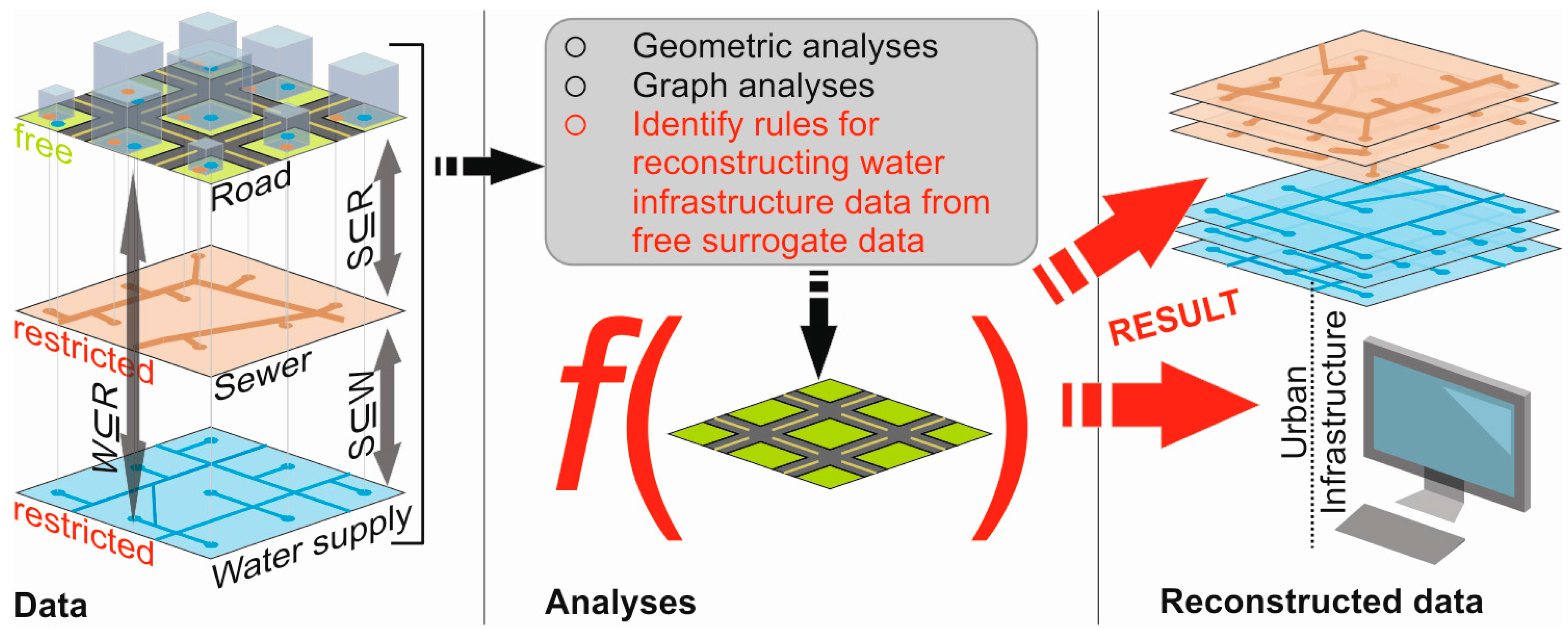
Figure 1 shows the overall vision of this work. In a first step the geometric- and graph-based characteristics (Figure 1: analyses column) of different network types on a multi-utility basis are identified (e.g., road, sewer, water supply (Figure 1: data column)). Based on the identified characteristics we assume to be able to reconstruct missing data of sewer and water supply network datasets with the help of surrogate data (e.g., road data) (see Figure 1: reconstructed data column).

The benefit of such a method would save significant time in data preparation. Virtual water networks could also potentially be automatically generated for benchmarking purposes of new designs and optimization algorithms [11].

The key to such an analysis, and a main focus of this work, is to identify the correlation of different infrastructure networks (i.e., streets and pipes). Likewise, identifying the potential characteristics, which may be used as a parameter for an algorithm to generate realistic water infrastructure models, is important. A first analysis has been performed in Mair, et al. [12], in which the main focus was to prepare easily accessible network data (the street network from OpenStreetMap) for the combined network analysis across street, sewer, and water supply networks. However, a detailed analysis containing the geometric and graph analytical indicators has not been previously performed. The aim of this paper is to close this gap by performing a detailed network analysis across the street, sewer, and water supply networks (on a multi-utility basis) to better understand the coherences in the design and layout and to identify important characteristics of the water infrastructure in urban areas. If such a spatial link can be identified, future work can focus on developing new approaches that complement missing data or even automatically generate the realistic and semi-artificial datasets of interlinked water infrastructure networks at a city scale. As accuracy of the surrogate data increases (e.g., the development data of streets), the use of this approach is not limited to the scientific community, but these sets may also be useful for stakeholders/planners for making decisions [13]. For example, it can be of interest for assessing future investments in infrastructure (e.g., assessing network structure uncertainties [14], spatial layout optimization [15], testing expansion strategies, or testing of rehabilitation strategies [16,17]). This work is, therefore, structured in two parts: (1) detailed statistical multi-utility analysis of three real-world test cases and identification of controlling parameters for network interdependencies; and (2) sensitivity analysis of the identified parameters.

2. Materials and Methods

In the scope of this work, street, water supply, and sewer networks are compared from different perspectives. To perform a sound analysis on all three network types, complete and detailed datasets are required for each network. Detailed datasets for street networks are easily accessible (e.g., from Google Maps or OpenStreetMap) and are already at a sufficient quality for automatic processing. To assess which information on water infrastructure can be deducted from the street data, case studies have investigated sufficient information sources covering the water supply and urban drainage network for the comparison. Data covering urban water infrastructure networks are available from existing EPANET2 [18] and SWMM5 [19] models for water supply and sewer networks, respectively. These datasets include detailed information (e.g., pipe width diameter, roughness coefficient, and slope information) of all network components required for state-of-the-art hydraulic modeling.

Each of the sets represents an infrastructure network system with a type-specific service within a defined service area. For a water supply network, the service is to supply water to specific locations, whereas in a sewer network, the service is to dispose storm and/or wastewater within the entire service area. The service areas of all three types of investigated networks may not be congruent and, therefore, the intersection of all service areas defines the area of interest on which the analyses are performed. Within this area, all required and detailed data must be available to develop a valid proposition about network similarities. 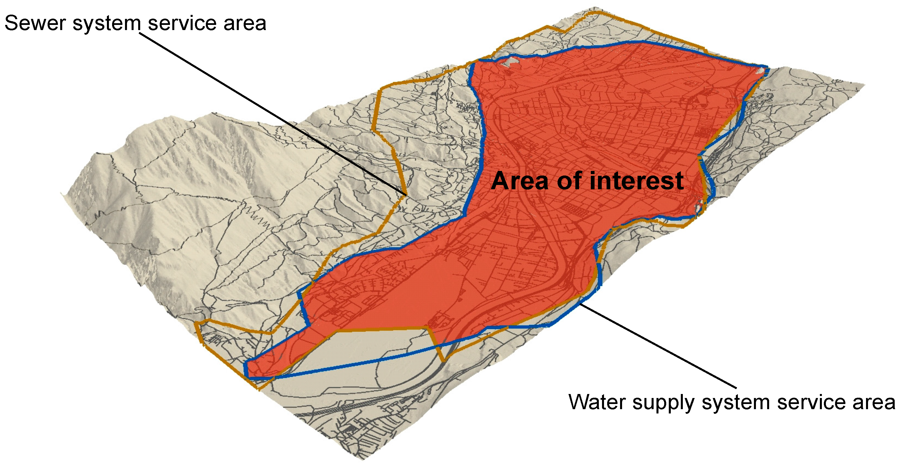Figure 2 shows the service area of the street, sewer, and water supply networks of an alpine city (in this work, this case study is called CS1). The solid-shaped polygon is the intersection of all three service area polygons and defines the area of interest regarding the data analysis.

A network correlation/similarity analysis can be performed in various ways. In this work, network layout and graph-based analyses are conducted. Under the scope of these two types, characteristics/indicators are identified to better understand the correlation of urban infrastructure.

2.1. Geometric Analysis and Parameter Sensitivity

Following the approach from Mair, et al. [12], a detailed analysis is performed for geometric network indicators over different network types (multi-utility basis). The analysis of different datasets includes a classification of the results depending on the different street types, pipe diameters, and conduit diameters. Street network data is easily accessible and often of good quality. In this work, street network data are used and downloaded from OpenStreetMap, including the specific street type of each element within the dataset (for five different types).

The exact street width and information about parking lots, pavements or additional lanes, for example, are not included in this data. To compensate for this lack of information, street widths depending on the street types are assumed (the assumed width in Section 3.2) and an additional width is included in the analysis resulting in a corrected width (the sum of the assumed and additional width). For sensitivity analysis, the parameter of the additional street width varies on both street sides from 0.5 to 5 m, while the related percentage of that which contains the infrastructure network is determined and analyzed (see Section 3.2). Analyses based on this assumption consider parallel pipes/conduits below a street. Once the corrected street areas are identified, street-type non-specific and specific geometric analyses can be performed by intersecting the geometric data of the different network types (see Section 3.3).

2.2. Graph Analysis

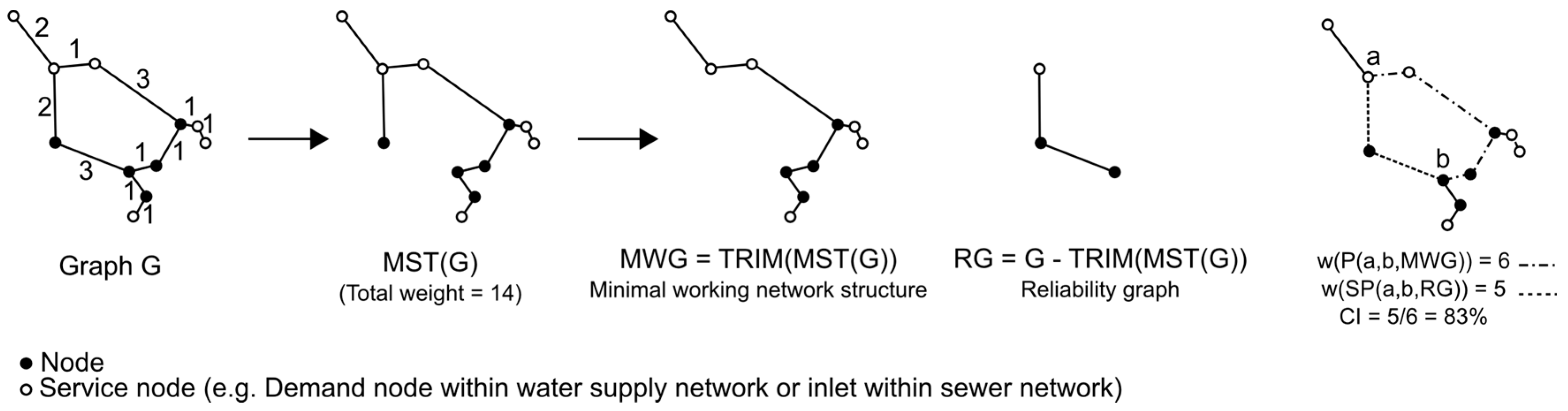
The network layout of a water supply or sewer system can be interpreted as an undirected connected graph, $G$, in which all link elements (e.g., pipes, pumps, conduits) are the edges ($E$) and all node elements (e.g., junctions, outlet, tanks, reservoirs) are the vertices ($V$) of a graph $G=\left(E,V\right)$. The weight of each edge is the function $w:E\to ℝ$, which maps each edge $e\in E$ to a value of $ℝ$. The weight of each edge is equal to the length of the corresponding link element in the real infrastructure network. Based on this representation, a graph-based analysis can be performed. Under the scope of this work, several different graph indicators are investigated: (1) total indicators, such as the total number of vertices ($\#V$) and the total number of edges ($\#E$); and (2) relative indicators, which are graph size independent. Since the latter indicator type is not as straightforward to compare to the total indicator type, the following definition is based on select informal and basic definitions of graph theory. The two indicators that are used in this work are then introduced.

A path $P$ of a graph $G$ is a sequence of vertices $\left(v_1,\dots , v_i\right)\in V^i$ in which each consecutive pair of vertices $\left(v_i,v_{i+1}\right)\in P$ is connected by an edge $e\in E$. The weight $w\left(P\right)$ of a path is the sum of all edge weights within the path. A shortest path (SP) is a path connecting two vertices within a graph in which the total weight is minimal. A cycle of a graph is a path in which the first and the last vertices are equal. A minimum spanning tree ($MST$) of a graph $G$ is a connected graph without cycles, which connects all vertices $MST=\left(E_{sub},V\right)\subseteq \left(E,V\right)=G$ and the sum of all edge weights is minimal. With the help of these basic definitions, the two indicators can be defined as the cycle (CI) and leaf indicator (LI). The authors of this work are aware of the immense diversity of graph measures and metrics in graph theory; however, in this work a new, innovative, and simple graph-based indicator is introduced with the focus on analyzing water infrastructure graphs.

2.2.1. Cycle Indicator (CI)

This indicator describes characteristics of the cycles (loops) within an infrastructure network and is often implemented for reliability purposes. Water supply and sewer networks are mostly realized with the aim of minimum construction cost. Crucial for the total construction cost of an infrastructure network is the total length of the network. If we disregard the aspect of reliability, the infrastructure network has a tree-like structure with minimum construction cost and service level. This is equivalent to a minimal working network structure (following called MWG). In a mathematical sense, this network is a generalized minimum Steiner tree [20] connecting all relevant nodes (these nodes are also known as Steiner terminals) in a given graph (e.g., street network graph) with a minimal network length, to guarantee the service offered by the water infrastructure network. The relevant vertices/nodes in a water supply network are all junctions with a demand greater than zero, and in a sewer network, all inlet nodes. Due to the high complexity (NP-complete) and, therefore, high computational runtime for finding such a tree, the following approximation with a time complexity of O(|E| log(|V|) + |V|²) is used for generating an MWG (|E| and |V| are the number of edges and vertices). Based on the MWG the cycle indicator (CI) can be evaluated. The overall runtime complexity of the MWG algorithm (Steiner tree approximation) is the sum of the MST algorithm complexity O(|E| log(|V|)) (Using Kruskal’s algorithm [21]) and TRIM algorithm complexity O(|V|²) (check each vertex if it is part of one unique edge and, if yes, deleting it). Additionally, more accurate, but also more computationally intense, approximations have been established [22]. In this work all analyses regarding the CI indicator are performed on datasets of water supply and sewer network graphs. Based on these graphs the generalized minimum Steiner tree is equivalent to a minimum spanning tree minus all non-terminal leafs. Hence, the choice of the approximation function has no impact on the results of CI.

The layout of a minimal working infrastructure network (Figure 3: $MWG$) is assumed to be equivalent to an MST of the graph (Figure 3: $MST\left(G\right)$) in which all leaves are removed that are not mandatory for the network service. All other edges are for redundant capacity, reliability, and part of a cycle (Figure 3: reliability graph). An MST of a graph does not necessarily need to be unique (e.g., graph G in Figure 3 has two different MSTs). By comparing the path length of the path connecting two vertices within the $MWG$ with the alternative shortest path length between the identical vertices in the reliability graph (RG), the fraction of the path length for building a cycle can be obtained. Equation (1) presents this comparison where $a \mathrm{and} b$ are two vertices of the graph $G$, $MWG\left(G\right)$ is a minimum spanning tree without leaves which are not relevant for the network service, and $P_{a,b}$ and $S{P}_{a,b}$ are a path and the shortest path of the graph $MWG$ and $RG$ connecting vertices a and b, respectively.

$$C{I}_{a,b}:=\frac{w\left(S{P}_{a,b}\left(RG\right)\right)}{w(P_{a,b}\left(MWG\left(G\right)\right))}(-)$$

(1)

By performing these steps for all possible tuple-combinations of vertices of graph $G$, all cycles/loops within an infrastructure network can be analyzed.

2.2.2. Leaf Indicator (LI)

A leaf of a graph is a path that is not part of any cycle. In urban water infrastructure networks, these paths correspond to household connections, pipes coming from the water source, and conduits leading to the waste-water treatment plant. Equation (2) shows the method employed for determining this indicator. $E_{sub}$ is the subset of all edges which are not part of any cycle. The fraction (LI) of leaves is equal to the total weight of all leaves divided by the total network weight.

$$LI:=\frac{{{\displaystyle \sum }}_{i=0}^{\#E_{sub}}w\left(e_i\right)}{{{\displaystyle \sum }}_{i=0}^{\#E}w\left(e_i\right)}(-)$$

(2)

2.3. Description of Case Studies (CS)

In this paper, we investigate three case studies in an alpine region with different network sizes, denoted as CS1 to CS3. For all case studies, information of the water supply (e.g., pipe diameter and length) and sewer (e.g., conduit cross section, roughness, and slope) systems are derived from hydraulic and hydrodynamic models, respectively. Street network data is downloaded from OpenStreetMap for the area of interest (intersecting the service area of the water supply and sewer network). Due to security concerns, we are not allowed to publish the exact layout of all case studies in this work. Therefore, all case studies are described by quantifying several characteristics.

Table 1. Case study properties.

	Row	CS1	CS2	CS3
Population (-)	1	120,000	13,000	11,000
Widest pipe diameter (mm)	2	600	500	250
Widest conduit diameter (mm)	3	2444	2130	1800
Lowest pipe diameter (mm)	4	25	31	30
Lowest conduit diameter (mm)	5	150	100	150
Total water supply network length (km)	6	217.67	64.2	61.9
Pipe length/inhabitant (m)	7	1.81	4.93	5.63
Total Sewer network length (km)	8	202.88	41.8	47.1
Conduit length/inhabitant (m)	9	1.69	3.22	4.28

shows initial properties of all three case studies. When using the population value as an indicator for the size of a service area, CS1 is the largest case study (resembling a medium-sized city) and CS2 and CS3 are nearly of equal size (resembling a small city/large village). All listed values should be seen as properties of the initial input datasets. The presented data reveals that, for all three hydraulic case studies, the level of detail (of the models) is approximately identical (e.g., the smallest pipe diameters range between 25 mm and 31 mm). Further, the water supply network in the city (CS1) has only a slightly higher length than the sewer network (7.43%). This difference is higher for the villages (CS2 and CS3; 53.59% and 31.42%, respectively). Within the city pipe/conduit length per inhabitant is much smaller in the city (for CS1, 2 m) compared to the villages (for CS2 and CS3, up to 6 m).

3. Results and Discussion

Geometric and graph-based analyses are performed for all three case studies and presented below with an interpretation. Similar to the structure of the described methods, the calculations of the area of interest are presented first. Next, the results of the detailed geometric analysis (evaluation based on street types and diameters of pipes and conduits) are shown, followed by graph-based analysis containing the indicators CI and LI.

3.1. Area of Interest

As described in the methods section, the area of interest is calculated by intersecting the service areas of the water supply and sewer network. This intersection is used for clipping the street network data.

Table 2. Area of interest properties for all case studies.

	Row	CS1	CS2	CS3
Area of interest—AI (km2)	1	25.14	5.88	5.35
Population density (Pop/ km2)	2	4774	2210	2056
Widest pipe diameter (mm)	3	600	305	250
Widest conduit diameter (mm)	4	2,440	2130	1800
Lowest pipe diameter (mm)	5	25	31	30
Lowest conduit diameter (mm)	6	150	100	150
Total water supply network length (km)	7	216.75	48.7	52.20
Pipe length/inhabitant (m)	8	1.81	3.74	4.75
Total sewer network length (km)	9	201.93	41.4	46.82
Conduit length/inhabitant (m)	10	1.68	3.19	4.26
Total street network length (km)	11	419.48	78.1	67.87

shows the identical properties of the input datasets, after clipping, according to the calculated area of interest. Using the area of interest as an indicator for describing the size of the systems, CS1 has the largest area with 25 km². CS2 and CS3 have nearly identical sizes resulting in close population densities when comparing these values with the population values in Table 1. Due to clipping the water supply and sewer network data to a common area of interest, some data is not regarded. The amount of clipped data is shown by comparing the total network length of the original input dataset (Table 1: rows 6 and 8) with that of the clipped data (Table 2: rows 7 and 9). Disregarded data of sewer networks is marginal for all three case studies. Neglected data of the water supply networks for the CS1 is also marginal. CS2 and CS3 show a higher deviation, with 24% and 15% of the data being clipped, respectively. This clipping results from the lower service area of the sewer networks. These clipped network zones are usually those parts of the sewer network in which not all inhabitants are connected to the sewer system, or in which long main trunks occur in the water supply network. Comparing the widest diameter of pipes occurring within the clipped (Table 2: row 3) and original (Table 1: row 2) water supply dataset, CS2 shows that many portions of the main trunks are not considered in this case. This is because of missing information of the sewer network in the identical area and long main trunks from the reservoir to the valley within the water supply network. Generally speaking, the service area of water supply systems is more likely to be larger when compared to the service area of the sewer system within the identical case study.

After clipping the street network datasets to the area of interest, Table 2 (row 11) shows that the obtained street network length is nearly twice as long as the sewer or water supply network within the identical case studies.

For the geometric analysis, all clipped datasets are used, and for the graph-based analysis, the original datasets are used for investigations.

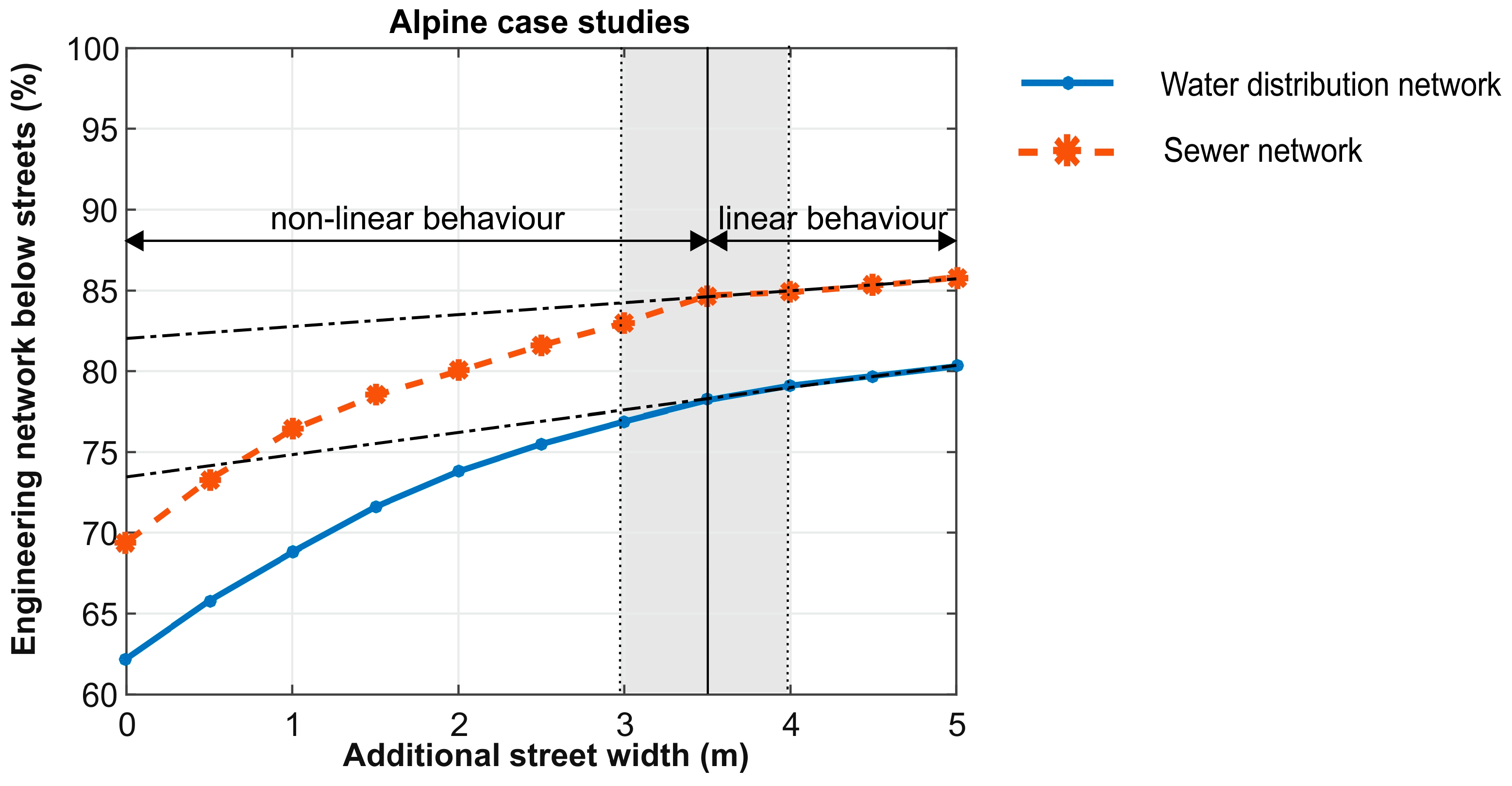
3.2. Parameter Sensitivity

The street network data used from OpenStreetMap does not contain information about parking lots, pavements, additional lanes, or roadside ditches. To compensate for this lack of information, the actual street width is increased by an additional street width. This is investigated in order to consider street parallel pipelines, which would not be identified with the initially-assumed street width from the literature (the assumed width in

Table 3. Assumed street width depending on street types.

Type	Motorway	Primary	Secondary	Tertiary	Other
Assumed width (m)	21	14	14	13	2
Corrected width (m)	28	21	21	20	9

).

Figure 4 shows the results of a sensitivity analysis where the correlation of additional street width and covered network length is investigated for the three alpine case studies. By adding additional street width starting from 0.5 m, the total water supply/sewer network length situated below the road increases in a non-linear manner. This increase results from the number of pipes or conduits, which are parallel to a street e.g., below a parking area. When all parallel elements (pipes or conduits) are within the corrected street width (assumed width + two times the additional street width), a re-increase of the street width results in a near-linear increase of the total water supply and sewer network lengths below a street (Figure 4—starting from 3.5 m of additional street width). This linear increase represents pipes/conduits crossing streets. These pipes should not be included in successive analyses. Therefore, the determined value for the additional street width is the point at which the curve changes from a non-linear increase to a linear increase (Figure 4—3.5 m of additional street width).

The outcome is similar for all case studies and reveals that a representative additional street width of around 3.5 m on both roadsides (in total 7 m) includes only parallel water infrastructure (for comparison see Figure 4). Based on this parameter, a corrected street width for each street type is determined.

Table 3 shows the different street types with the assumed and corrected street widths. The latter includes an additional width of 3.5 m on each street side, determined from the previous analysis. The street type “Other” includes streets with the street types “service”, “residential”, and “unclassified”. These types have nearly identical widths; therefore, these types are merged into one category. For further analysis, the corrected street widths are used.

3.3. Geometric Analysis

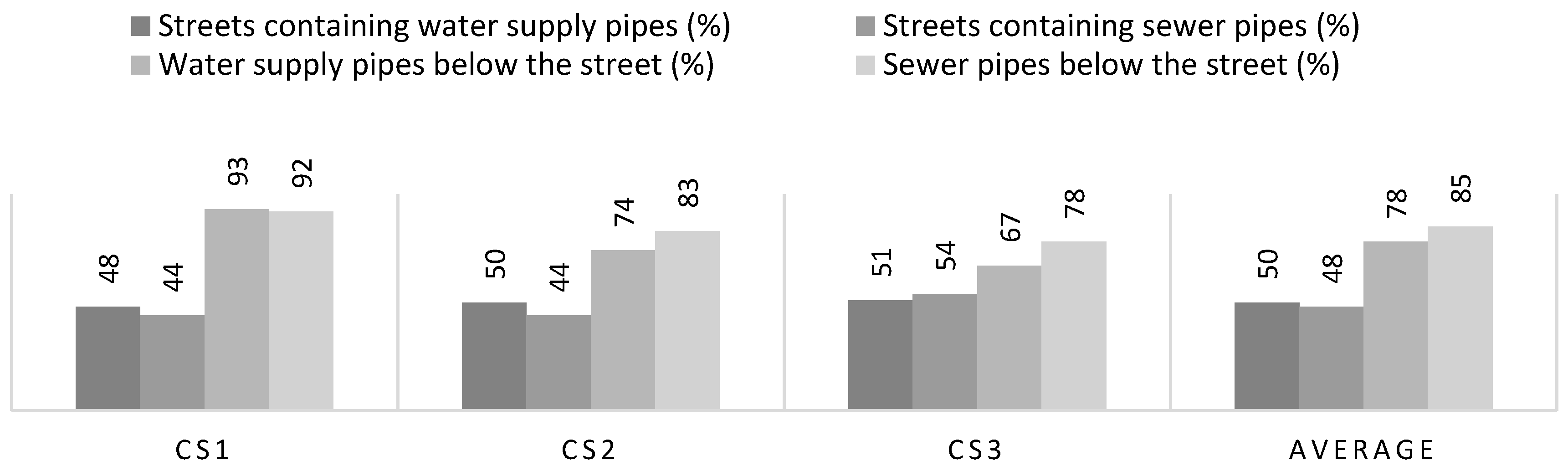
Figure 5 shows selected general geometric results from all three case studies. Compared to the geometric analysis performed in Mair et al. [12], in which a pipe or conduit is identified to be below a street independently of the length, in this work, the results depend on the pipe or conduit length. The average values show that approximately 50% of the street network contains 78% of the water supply or sewer network. Due to the limited area for water supply and sewer systems in high-density areas, this value is increasing, demonstrated by CS1 with a value exceeding 90%.

Table 4. Fraction of street types in a street network.

Case Study	Motorway	Primary	Secondary	Tertiary	Other
CS1	6.12	7.67	2.60	7.81	75.80
CS2	0.35	6.89	2.62	8.37	81.77
CS3	2.97	5.48	7.88	3.78	79.88

shows the fraction of different street types within the street networks (clipped by the area of interest). Only between 10% and 20% of the total street network length are motorways, primary, secondary, or tertiary streets. The remaining streets are categorized as others and include service, residential, and unclassified streets with the same geometric characteristics.

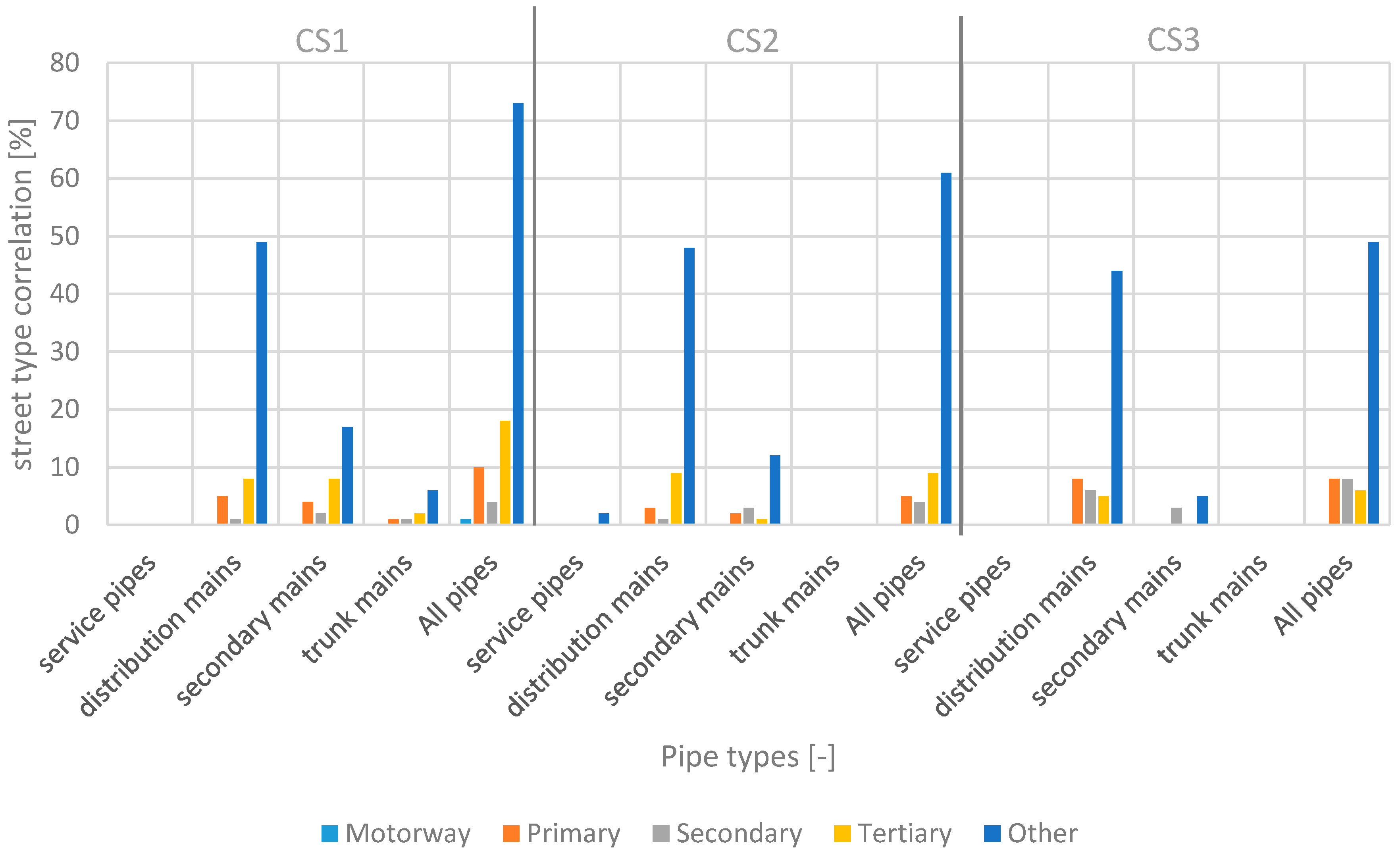
Investigations into the fraction of pipe diameters and type of the street are presented in Figure 6. Following Trifunovic [23], pipes are classified according to their diameter ($d$ in mm) and usage, i.e., into trunk mains ($d\ge 400$ ), secondary mains ($200\le d<400$), distribution mains ($80\le d<200$), and service pipes ($d<80$).

The columns “All pipes” in Figure 6 and columns “d > 0” in Figure 7 show the fraction of the pipe and conduit classification within a water supply and sewer network independent of the street types, respectively. By contrast, all other columns show the fraction of pipes and conduits of the entire network length in correlation with the five different street types (Figure 6 and Figure 7). These results are also presented in form of a table in Appendix A.

Below a motorway, only one percent of all pipes of a water supply system are placed. These pipes are mostly only crossing the motorway. Independent of the diameter, between 49% and 72% of a water supply network are found below the street type “Other”. Approximately 50% of the diameters in this category display a diameter between 80 mm and 200 mm, accounting for the class “distribution mains”. Generally speaking, approximately 60% of water supply network pipes are distribution mains. The fraction of service pipes is a sign of the level of detail of the network data (household connection included or not).

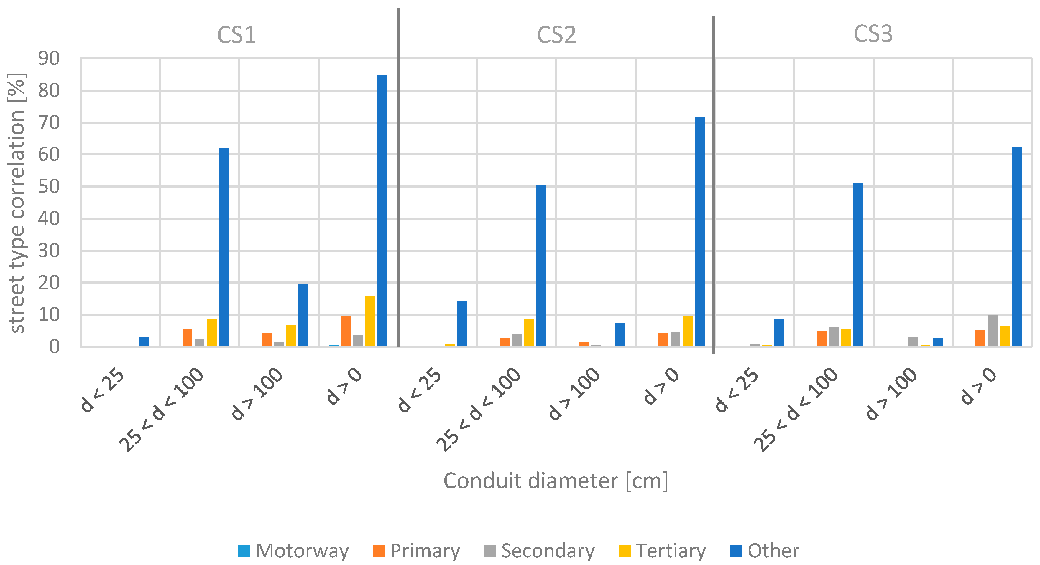
Similar to the classification of pipes according to usage in water supply systems, a classification for conduits (three different classes on the basis of Gujer [24]) within sewer systems is performed. Figure 7 shows the fraction of conduit diameters according to specific street types. The major portion (between 62% and 85%) of a sewer network is below a street of type “Other”, less than 10% is below primary/secondary streets, and less than 1% is below motorways.

The results of this analysis reveal a strong correlation between street network data and urban water infrastructure networks. Furthermore, the presented results can be used for complementing missing spatial network information (missing pipes) when datasets are of poor quality. Further, the results can be used for developing and validating complementary approaches or generation procedures using street network data as the input and generating entire sets of semi-artificial water infrastructure networks. In developing countries, water network information might even be missing. In this case, a possible water infrastructure layout can be created with such a generation procedure.

A correlation between street network types and conduit/pipe diameter could not be found in this analysis. Due to the missing construction year information in the street network dataset, information about pipe/conduit construction year and roughness cannot be extracted. However, planning rehabilitation measures for water infrastructure, information of the construction age is an important parameter [25]. Such historic network information is harder to gather than the actual state of a system. The results of this study can potentially also contribute to close this information gap by using historic street network information (derived from historical orthophotos) as the basis for network reconstruction of historical network states.

3.4. Graph Analysis

Table 5. Results of the graph analysis for water supply networks.

	CS1	CS2	CS3	Average
#Nodes (-)	7128	790	452
#Edges (-)	7600	878	602
85% percentile of CI (%)	49.84	58.53	60.67	56.35
LI (%)	11.18	12.81	11.89	11.96

and

Table 6. Results of the graph analysis for sewer networks.

	CS1	CS2	CS3	Average
#Nodes (-)	5395	1232	1700
#Edges (-)	5756	1248	1710
85% percentile of CI (%)	34.98	19.25	29.29	27.84
LI (%)	28.62	80.83	64.68	58.04

show the results of all absolute and relative graph theory based analyses for water supply and sewer systems, respectively. These analyses are performed on the original dataset for the water supply and sewer network, in which no clipping according to the area of interest was performed. The reason for not clipping the data is that only the graph structure of the system should be analyzed with no geometric effects of other infrastructure network graphs.

The results show that the leaf indicator (LI) within a water supply network is approximately 12% of the total network length (Table 5: LI). All other parts of the network are a part of one or more loops. Independent of the case study size, nearly the identical fraction can be identified. The fact that 88% of a water supply network is looped reflects the constraints on a water distribution system: not to fail in any circumstances.

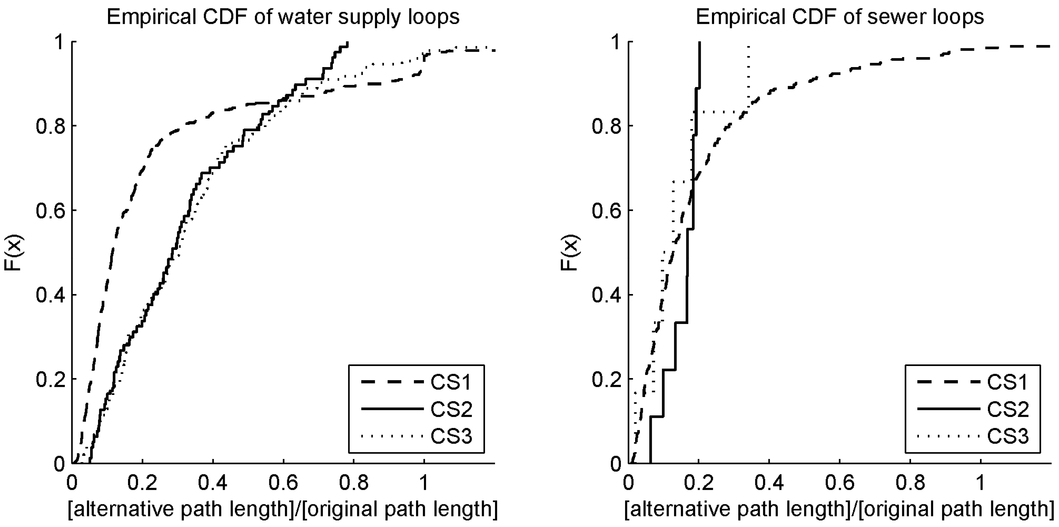
Evaluating the cycle indicator (Table 5: CI) shows that 85% of all loops within a water supply network are constructed by including an alternative path between two service nodes, which is only up to 60% of the original path length in the MWG. In short, pipes for reliability are shortcuts for up to 40% of the distance between two service nodes compared to the path within the MWG. The plot of the empirical cumulative distribution function (CDF) of this indicator (Figure 8: left) shows that in CS1, the gradient is much steeper when compared to CS2 and CS3. This steeper gradient results from the high degree of looping and urbanization in CS1, in which 93% of all pipes are below a street.

The identical analysis was performed for sewer systems (Table 6). Results indicate that the leaf indicator (LI) within a sewer network is between approximately 30% and 80%, with a mean value of 58%. These values show that the investigated sewer systems have fewer loops when compared to the water supply systems (Figure 8: right—note, only a few data points are available for CS2 and CS3). These low values result from the higher tolerance of system failures for sewer systems. CS1 has a leaf indicator of 29%, which results from the higher population density and a higher meshed network layout when compared to CS2 and CS3. Moreover, CS1 has a combined sewer system with the main aim of preventing flooding of the system within highly urbanized areas during heavy rain events and to treat polluted surface runoff at the wastewater treatment plant during most rain events. In addition to the construction of additional storage volumes in combination with combined sewer overflows within such systems, this combined system can be maintained by constructing alternative flow paths (closing loops) to better distribute local storm water runoff. By contrast, CS2 and CS3 have a lower population density; in the urban areas, therefore, more pervious areas are available for the construction of infiltration sites. The piped sewer system is, therefore, not highly stressed during heavy rain events and the system redundancy (loops) can be limited.

However, when loops in such systems occur, more than 85% of all loops are constructed to include an alternative path between two service nodes for which the length is up to 30% of the original path length (Table 6: CI and Figure 8: right).

3.5. Applications of the Results Obtained from the Graph and Geometric Analyses

The analyses of this work are performed in order to better understand the correlation of different urban infrastructures and to identify potential surrogate data sources (Does the street network data help to better understand and describe the water infrastructure or does knowledge on, e.g., the water supply network support improving drainage data?). The obtained results also improve the understanding of urban network infrastructure from an integrated point of view and can be fundamental for different research purposes, like data verification, data completion, or even the entire generation of feasible datasets. For data complementation for deterioration modelling and data verification the benefits of a multi-utility approach were shown in [25]. Additionally, for systematically testing of alternatives for future water infrastructure planning based on land-use master plans [26], the obtained results of this work can be essential.

Another application of the obtained results is the enhancement of existing water network generation algorithms to create so-called virtual or semi-virtual networks. In this regard the results from this work enable identifying and quantifying potential parameters and showing the applicability of the foreseen methods for network generation. Further investigations on developing, testing, and validating such an algorithm are previously successfully applied and presented [14]. In that work, design criteria and hydraulic performances of the virtual systems are also compared to those of the assumed unknown real system. It is shown that, with the stochastic generation process, hydraulic pressure differences in water supply models lower that ±4 m compared to the real system could be achieved for design loads.

4. Summary, Conclusions, and Outlook

In this manuscript, correlations in the urban infrastructure networks in the field of urban water management are analyzed in order to better understand the correlation of different urban infrastructures and to identify potential sources for surrogate data.

The investigation is split into two main parts: a geometric analysis and a graph-based analysis. All calculations were performed on three case studies with different sizes in which complete and detailed datasets of street, water supply, and sewer networks are available. The first case study has 120,000 inhabitants, and the other two case studies have approximately 13,000 and 11,000 inhabitants. To strengthen the validity of the obtained results, future work will also focus on including more, and international, case studies.

The results of geometric-based analyses showed a strong correlation between street networks and the urban water infrastructure (water supply/sewer network). On average, 50% of the street network length correlates with 80%–85% of the total water supply/sewer network. Urban water infrastructure networks are developed and constructed similar to a street network layout when using all streets of type “Others” (analyzed with OpenStreetMap data). A correlation between the pipe/conduit diameter and street type was not found. Due to the missing construction year information in the street network dataset, information covering the material and age of the pipes/conduits cannot be extracted.

The graph-based analysis showed that up to 12% and 80% of a water supply and sewer system, respectively, are not part of any loops. The other parts of the network are completely looped. In total, 85% of all loops within a water supply and sewer system are constructed by finding an alternative path between two service nodes for which the path length is up to approximately 56% and 28% when compared to the original path, respectively.

The focus was on identifying and quantifying significant network indicators, which are potentially useful as parameters for further applications. Potential application of the findings (e.g., deterioration modelling, future infrastructure planning, data complementation, or virtual network generators) were also identified and outlined. Especially for network generation algorithms, we investigated and evaluated graph-based indicators (leaf indicator and cycle indicator), which are fundamental for the development of such approaches. We observed that graph-based indicators are more useful as input parameters for such algorithms, whereas the geometric indicators are more suitable for validation. Statistically quantifying these indicators enables the development and validation of infrastructure networks (semi-virtual sewer and water supply network datasets) and the generation of algorithms for further use (e.g., a benchmark set to optimize algorithms and new hydraulic solver implementations). Such algorithms will consist of two parts: (1) network layout algorithms that can be seen as a reverse function of the cycle indicator; and (2) fulfilling hydraulic properties, which is an engineering design/optimization problem.