Improvements to Runoff Predictions from a Land Surface Model with a Lateral Flow Scheme Using Remote Sensing and In Situ Observations

Abstract

Like most land surface models (LSMs) coupled to regional climate models (RCMs), the original Common Land Model (CoLM) predicts runoff from net water at each computational grid without explicit lateral flow (LF) schemes. This study has therefore proposed a CoLM+LF model incorporating a set of lateral surface and subsurface runoff computations controlled by topography into the existing terrestrial hydrologic processes in the CoLM to improve runoff predictions in land surface parameterizations. This study has assessed the new CoLM+LF using Earth observations at the 30-km resolution targeted for mesoscale climate applications, especially for surface and subsurface runoff predictions in the Nakdong River Watershed of Korea under study. Both the baseline CoLM and the new CoLM+LF are implemented in a standalone mode using the realistic surface boundary conditions (SBCs) and meteorological forcings constructed from remote sensing products and in situ observations, mainly by geoprocessing tools in a Geographic Information System (GIS) for the study domain. The performance of the CoLM and the CoLM+LF simulations are evaluated by the comparison of daily runoff results from both models with observations during 2009 at the Jindong stream gauge station in the study watershed. The proposed CoLM+LF, which can simulate the effect of runoff travel time over a watershed by an explicit lateral flow scheme, more effectively captures seasonal variations in daily streamflow than the baseline CoLM.

1. Introduction

Regional climate models (RCMs) that have been used to reproduce past and recent climate features are expected to provide credible predictions of future climate changes and impacts at regional or local scales. For the predictability of RCMs, the coupled models need more realistic and accurate calculations for interactions between the land surface and the atmosphere [1]. The Intergovernmental Panel on Climate Change (IPCC) also addressed the need for improvements to terrestrial land surface parameterizations in land surface models (LSMs) coupled to RCMs [2]. As the climate and hydrology modeling studies have developed toward physical sophistication and high resolution, LSMs coupled to RCMs have improved land surface parameterization schemes by incorporating sophisticated process interactions in the terrestrial hydrologic cycle [3,4,5,6,7,8,9,10]. However, some unrealistic parameterizations for terrestrial hydrologic schemes in LSMs have a direct or indirect influence on the complex and dynamic responses of land surface processes, which may cause serious errors in both terrestrial water and energy predictions.

The fact that most land surface parameterizations are currently limited to vertical fluxes in each single grid column may negatively affect the model’s predictions for terrestrial water and energy processes, especially because the existing terrestrial hydrologic schemes in most LSMs are incapable of representing the lateral water movement induced by topographic features. As incoming precipitation is divided into evapotranspiration, soil moisture, surface and subsurface runoff by land surface processes in LSMs, runoff plays an important part in the terrestrial water budget. However, runoff is estimated just by the soil water budget without topographically controlled surface and subsurface flow schemes in most LSMs. Moreover, surface runoff used for neither soil moisture nor subsurface runoff calculation as the boundary condition results in a mass balance error in the terrestrial water cycle. The infiltration rate calculations do not take into consideration the role of surface flow depth, which can cause errors in both infiltration and surface flow calculations [11,12,13]. Such unrealistic and simplified parameterizations in the terrestrial hydrologic scheme may affect other key components in land surface water and energy cycles, limiting the predictability of LSMs.

The Common Land Model (CoLM), a Soil–Vegetation–Atmosphere Transfer (SVAT) model [14], already coupled to the mesoscale Climate–Weather Research and Forecasting model (CWRF), has been developed and updated for sophisticated land surface processes. The CWRF has built-in modules for realistic Surface Boundary Conditions (SBCs) and is the most comprehensive of the weather and climate models [15,16,17]. The CWRF’s responses to various subgrid topographic representations and parameter selections were examined [18,19]. A scalable soil moisture transport scheme was developed for representing subgrid topographic control in land–atmosphere interactions of the CWRF [20,21]. The CWRF simulations were evaluated based on a continuous integration for the period 1979–2009 using a 30-km grid spacing over the North American domain [22]. The model improvement and performance of the CWRF were evaluated especially for possible impacts of precipitation, temperature, radiation, and extreme events’ occurrence and magnitude to help with future climate projection [23]. Also, many studies [6,7,8,9,14,24,25,26,27,28] have evaluated the performance of the CoLM simulations in a standalone mode by the observational forcing data. Nonetheless, the mesoscale simulations of the CoLM at the 30-km resolution are found to still have problems in the terrestrial hydrologic scheme, especially streamflow runoff predictions. Choi et al. [10] have therefore developed a conjunctive surface-subsurface flow (CSSF) model based on a one-dimensional (1D) diffusion wave model for the surface flow routing scheme coupled with the 3D volume averaged soil-moisture transport (VAST) model for water flux in unsaturated soils [21]. However, the CSSF model cannot be widely implemented yet for watersheds all around the world because the VAST model requires closure parameterizations by regional estimates of subgrid and lateral soil moisture fluxes for each local watershed.

Based on an assumption that the lateral soil moisture movement may not be a major water flux in large spatial scale simulations, this study has focused on incorporating a routed surface flow scheme and an unrouted subsurface lateral runoff scheme into the existing 1D soil moisture transport formulation to evaluate the influence of a lateral flow scheme on runoff predictions in the CoLM. A new version of the CoLM, named CoLM+LF, is proposed in this study as it can explicitly route surface runoff from excess water of both infiltration and saturation, and estimate subsurface runoff induced by topographic controls. This study has implemented both the baseline CoLM and the new CoLM+LF at the CWRF 30-km grid resolution, focusing on surface and subsurface runoff predictions because the terrestrial hydrologic parameterizations including the runoff scheme must be tested and evaluated at the same resolution as the coupled climate models.

The principal aim of this study is to assess the improvement to runoff predictions from the new CoLM+LF with a lateral flow scheme using the best Earth observation data possible for model predictability. For evaluating the performance of runoff results simulated from both the baseline CoLM and the new CoLM+LF, this study has selected a watershed under study, the Nakdong River Watershed in Korea. All the CoLM and the CoLM+LF schemes were implemented at 30-km grid points in this study watershed without any downscaling and upscaling schemes for exchanges between the atmosphere and the land surface. For such direct applications of both the CoLM and the CoLM+LF, this study has constructed a set of realistic SBCs and meteorological forcing data based on high-quality Earth observations at the finest possible resolution from multifarious sources such as remote sensing products (see Section 3.2 for details), photography images, in situ observations, scanned and digitized maps, etc. for the study domain at 30-km (0.25°) resolution on the geographic coordinate system following Choi [29,30]. The raw data at finer resolutions were transformed into SBCs on the 30-km spacing grids in the study domain mainly by geoprocessing tools in a Geographic Information System (GIS), ArcGIS (ESRI, Redlands, CA, USA). Most meteorological forcing data to drive both the CoLM and the CoLM+LF simulations in a standalone mode were spatially interpolated onto the 30-km computational grids by the Inverse Distance Weighting (IDW) method in ArcGIS from observations at 19 gauge stations managed by the Korea Meteorological Administration (KMA) around the study watershed. For the performance assessment of the terrestrial hydrologic schemes in predicting runoff by the goodness-of-fit test, the results from both the CoLM and the CoLM+LF simulations through the sensitivity analysis of key parameters for runoff variables were compared with daily streamflow discharges during a year of 2009 observed at the Jindong stream gauge station managed by the Ministry of Land, Infrastructure, and Transport (MOLIT) near the drainage outlet of the Nakdong River Watershed, Korea. It is expected that the proposed CoLM+LF with a lateral flow scheme using realistic Earth observations can more effectively generate daily streamflow variations compared with the baseline CoLM runoff results from the local net excess water flux in each grid when ignoring the role of surface flow depth over the watershed, as most current LSMs do.

2. Model Description

Although the CSSF incorporates the 3D VAST for improvements to terrestrial hydrologic schemes, the implementation of the 3D VAST model requires five key parameters for the dependence of soil moisture variability or terrain features on the mean moisture flux, which should be regionally estimated for each watershed. Owing to a lack of applicable regional parameters for the use of the 3D VAST model, this study has proposed a new version of the CoLM, named the CoLM+LF, to improve runoff predictability. Hence, a set of topographically controlled surface and subsurface flow schemes have been combined with the existing 1D soil water transport scheme in the baseline CoLM. A sensitivity analysis of key parameters for runoff variables in both the baseline CoLM and the new CoLM+LF is also presented in this study.

2.1. Baseline Runoff Scheme in the CoLM

Surface runoff $R_s$ is generated by Hortonian runoff [31] due to infiltration excess and Dunnian runoff [32] induced by saturation excess as:

$$R_s=\underset{Hortonian}{\underbrace{(1-F_{imp})\max [0,Q_w-I_{\max }]}}+\underset{Dunnian}{\underbrace{F_{imp}{Q}_w}},$$

(1)

where $F_{imp}$ is the impermeable area fraction of the saturated area and the frozen area. $Q_w$ is the available water supply rate such as rainfall, dewfall, and snowmelt rate on the surface. $I_{\max }$ is the maximum potential infiltration rate.

In the CoLM, subsurface runoff $R_{sb}$ comprises three components as:

$$R_{sb}=R_{sb,bas}+R_{sb,dra}+R_{sb,sat},$$

(2)

where $R_{sb,bas}$, $R_{sb,dra}$, and $R_{sb,sat}$ denote subsurface runoff components from baseflow, bottom drainage, and saturation excess, respectively. The bottom drainage contribution to subsurface runoff is negligible when the actual bedrock is located within the model soil layers under the exponentially decay profile of the hydraulic conductivity. The saturation excess runoff rarely occurs by incorporating a maximum surface infiltration limit condition and the effective hydraulic conductivity function at the interface of unfrozen areas from Choi and Liang [9]. In this study watershed under such conditions, the baseflow is almost comparable to the whole subsurface runoff.

After Sivapalan et al. [33], the baseflow is calculated by the subsurface saturated lateral runoff equation based on the TOPMODEL [34] as:

$$R_{sb,bas}=\frac{\zeta K_s(0)}{f}{e}^{-\overline{\lambda }}{e}^{-f{z}_{\nabla }},$$

(3)

where $\zeta$ is an anisotropic ratio of the lateral to the vertical hydraulic conductivities, $K_s(0)$ is the saturated hydraulic conductivity on the surface of the top soil layer, and $f$ is the decay factor of the saturated hydraulic conductivity. $\overline{\lambda }$ is the grid-averaged topographic index defined as $\lambda =\ln (a/\tan \beta )$ where $a$ is the drainage area per unit contour length and $\tan \beta$ is the local surface slope. $z_{\nabla }$ is the water table depth. Because the topographic index $\lambda$ has uncertainties in the regional and continental studies where the digital elevation model (DEM) data are generally available at coarse resolutions [35], a simplified parameterization of Equation (3) was used in some models [6,7,9,25] as:

$$R_{sb,bas}=R_{sb,\max }{e}^{-f{z}_{\nabla }},$$

(4)

where a single calibration parameter $R_{sb,\max }$ is the maximum baseflow coefficient representing $\zeta K_s(0)e^{-\overline{\lambda }}/f$.

2.2. Lateral Flow Runoff Scheme in the CoLM+LF

For the interaction between surface and subsurface runoff components, the new scheme considers the influence of overland flow depth on both infiltration rate and surface runoff. Total available water supply rate $Q_t$ on the surface is computed by incorporating the surface flow depth $h$ during a computational time $\mathsf{\Delta }t$ into the available water supply rate $Q_w$ as:

$$Q_t=Q_w+h/\mathsf{\Delta }t,$$

(5)

Hence, the net surface runoff $R_n$ as a result of water exchange between surface and subsurface is

$$R_n=(1-F_{imp})\max [0,Q_t-I_{\max }]+F_{imp}{Q}_t-h/\mathsf{\Delta }t,$$

(6)

In addition, the CoLM+LF model utilizes the 1D non-inertia diffusion wave equation for a surface flow routing scheme as:

$$\frac{\partial h}{\partial t}+c_d\frac{\partial h}{\partial x_c}=D_h\frac{{\partial }^{2}h}{\partial x_c^2}+R_n,$$

(7)

where $t$ is time and $x_c$ is a flow direction coordinate. $c_d$ is the diffusion wave celerity and $D_h$ is the hydraulic diffusivity. Note that the spatial and temporal variation of the surface water simulated by the 1D diffusion wave model in Equation (7) depends on the net water exchange flux $R_n$ between surface and subsurface in Equation (6).

The surface flow rate $Q_s$ using the Darcy–Weisbach formula can be written as:

$$Q_s=B{h}^{3/2}\sqrt{\frac{8g}{f_d}(S_o-\frac{\partial h}{\partial x_c})},$$

(8)

where $B$ is the flow cross-section width and $g$ is the gravitational acceleration. $f_d$ is the Darcy–Weisbach friction resistance coefficient calculated for flow regimes such as laminar, transition, or turbulent, respectively, based on the Reynolds number of the surface flow. $S_o$ is the bottom slope in the flow direction.

Baseflow Equations (3) and (4) in the baseline CoLM are incapable of representing the frozen soil area and surface macropore effects as well as the hydraulic conductivity variation with soil textures for different layers. Moreover, both equations may either fail to capture observed recession curves or produce unrealistic remaining soil moisture content, as demonstrated in Choi and Liang [9]. Starting with the basic assumptions in TOPMODEL, therefore, the saturated lateral flow $q_b$ at a depth $z$ beneath a water table can be written as:

$$q_b(z)=F_{liq}(z)\zeta K_{s_z}(z)\tan \beta ,$$

(9)

where $F_{liq}$ is the unfrozen part of soil water and $K_{s_z}$ is the vertical saturated hydraulic conductivity.

The baseflow runoff $R_{sb,bas}$ for a grid cell area A is calculated by integrating Equation (9) through the entire saturated soil layers and along the channel length L connected to the grid outlet as:

$$R_{sb,bas}=\frac{Q_b}{A}=\frac{{\displaystyle {\int }_L}{\displaystyle {\int }_{z_{\nabla }}^{z_N}}{q}_{b}dzdL}{A}=\frac{{\displaystyle {\int }_L}{\displaystyle {\int }_{z_{\nabla }}^{z_N}}{F}_{liq}(z)\zeta K_{s_z}(z)\tan \beta dzdL}{A}=\frac{{\displaystyle \sum _{k=j}^{N}T(k)}\tan \beta \cdot L}{A},$$

(10)

where $Q_b$ is the total baseflow from a grid cell. $T(k)={\displaystyle {\int }_{z_{k-1}}^{z_k}{F}_{liq}(z)\zeta K_{s_z}(z)dz}$ is a transmissivity varying nonlinearly with depth between vertical coordinates $z_k$ and $z_{k-1}$ of the layer $k$ where $z_{k-1}$ is replaced with $z_{\nabla }$ for the interface layer $j$ with the water table. $N$ is the total number of soil layers. To prevent Equation (10) from producing an unrealistic (negative or less than the residual) value for soil moisture content, a layer baseflow $q_b(k)$ for each discrete layer $k$ below the water table $z_{\nabla }$ is finally determined as:

$$q_b(k)=\min \left[\frac{T(k)\tan \beta \cdot L}{A},\frac{[{\theta }_{liq}(k)-{\theta }_r(k)]\mathsf{\Delta }{z}_k^{\prime }}{\mathsf{\Delta }t}\right],$$

(11)

where $\mathsf{\Delta }{z}_k^{\prime }=\{\begin{array}{ll}{z}_k-z_{\nabla }\hfill & \mathrm{for}k=j\hfill \\ z_k-z_{k-1}\hfill & \mathrm{for}k=j+1toN\hfill \end{array}$. ${\theta }_{liq}$ is the liquid soil moisture content and ${\theta }_r$ is the minimum soil moisture content for residual water in a soil.

The liquid water ${\theta }_{liq}(k)$ for each soil layer $k$ should be updated by the layer baseflow $q_b(k)$ for mass conservation as:

$${\theta }_{liq}(k)={\theta }_{liq}(k)-\frac{q_b(k)\mathsf{\Delta }t}{\mathsf{\Delta }{z}_k},$$

(12)

where $\mathsf{\Delta }{z}_k=z_k-z_{k-1}$ is a layer thickness for the layer $k$.

3. Model Implementation

The new CoLM+LF model has incorporated a set of topographically controlled surface and subsurface flow schemes into the existing terrestrial hydrologic representation in the baseline CoLM. The performance of both the baseline CoLM and the new CoLM+LF in predicting runoff was evaluated over the second-largest watershed on complex terrain in Korea to study the impact of lateral flow induced by topography using the 30-km computational grid mesh targeted for regional applications. The model experiments were performed in a standalone mode for which both the CoLM and the CoLM+LF were driven by the realistic SBCs and meteorological forcing data at the 30-km grid scale, constructed by applications of Earth observation data and GIS in this study.

3.1. Study Watershed

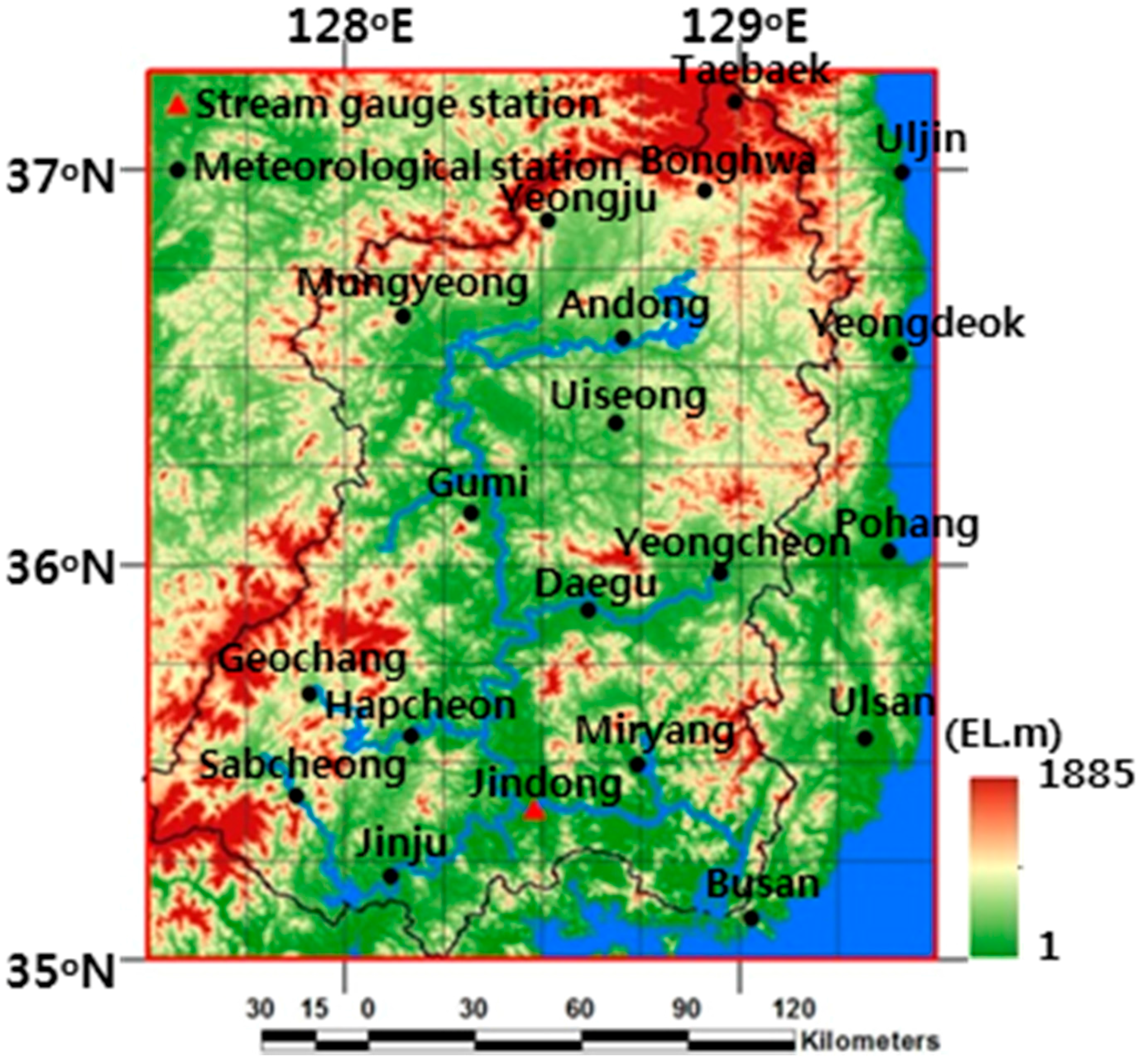
The Nakdong River Watershed with high topographic heterogeneity in Korea was selected under study to evaluate the performance of the baseline runoff simulation in the CoLM and the lateral flow adopted runoff simulation in the CoLM+LF at the 30-km resolution. Figure 1 shows the study domain comprising 72 (8 × 9) computational grid cells at 30-km (0.25°) horizontal spacing overlaid with the main streamline and the watershed boundary of the Nakdong River on the geographic coordinate system. The Nakdong River Watershed is located between 127°29′~129°18′ E and 35°03′~37°13′ N with the size of 23,384.21 km² and the main channel length of 510.36 km. The Nakdong River flows from the Taebaek Mountains over the north region to the South Sea. The terrain elevation ranges from 1 to 1885 EL.m over the watershed, and the width of the river ranges from only a few meters in its upper reaches to several hundred meters towards its estuary. Major land cover types are comprised of irrigated cropland/pasture, cropland/woodland mosaic, savanna, and mixed forest in the USGS land cover classification. A stream gauge station is located at the Jindong Bridge where daily streamflow discharges were measured in 2009 by the MOLIT. There are 19 meteorological gauge stations managed by the KMA around the study watershed for hourly or daily observations. See Section 3.3 for details on observations and meteorological forcing data in the study domain.

3.2. Surface Boundary Conditions

This study has constructed a set of primary SBCs from high-quality and -resolution observational data over the Nakdong River Watershed. The primary SBCs required for the CoLM and the CoLM+LF implementations comprise three groups of SBC datasets related to vegetation, terrain, and flow direction features on the 30-km spacing grids transformed from various Earth observations at the finest resolution possible for the study domain.

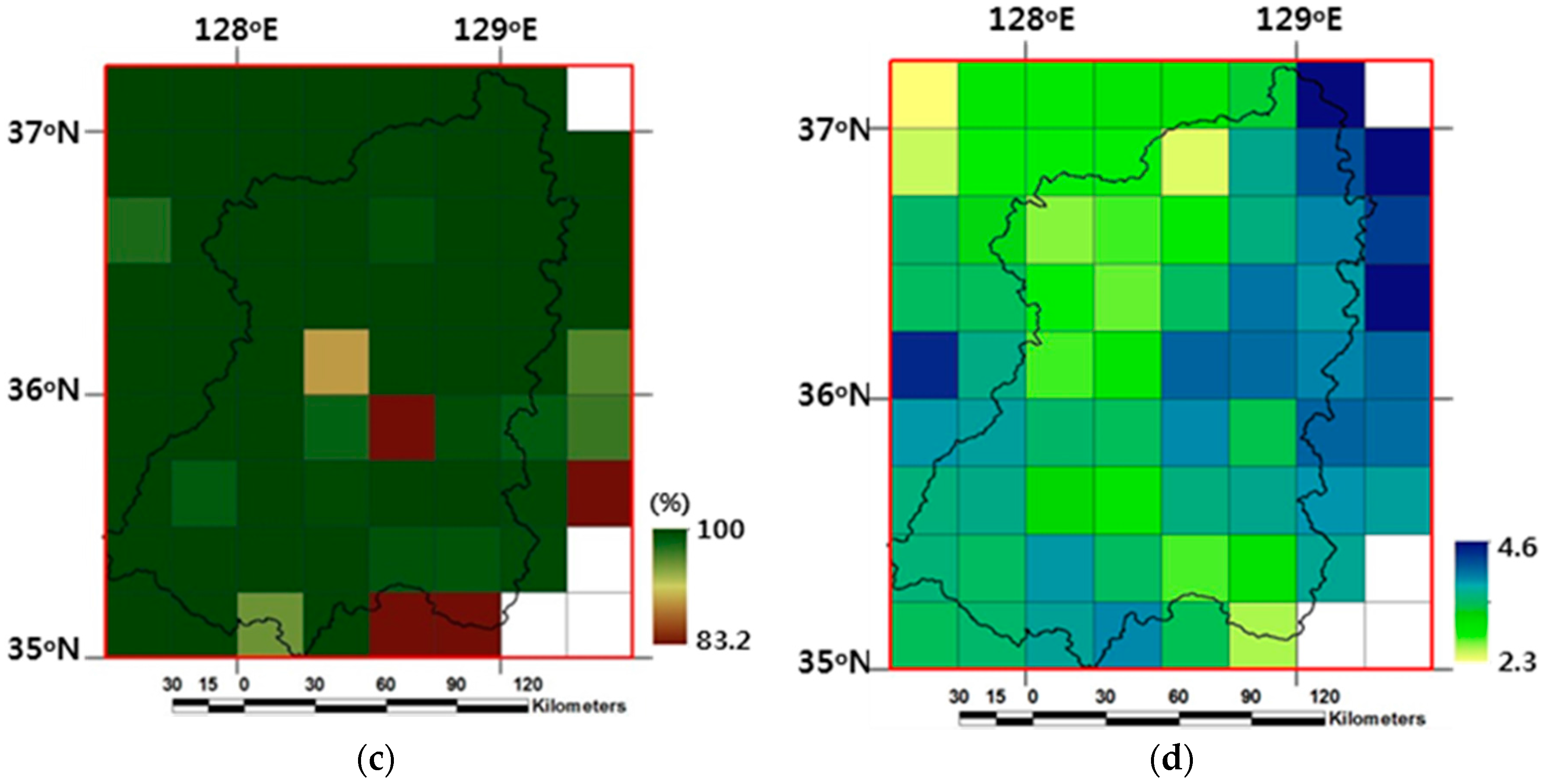
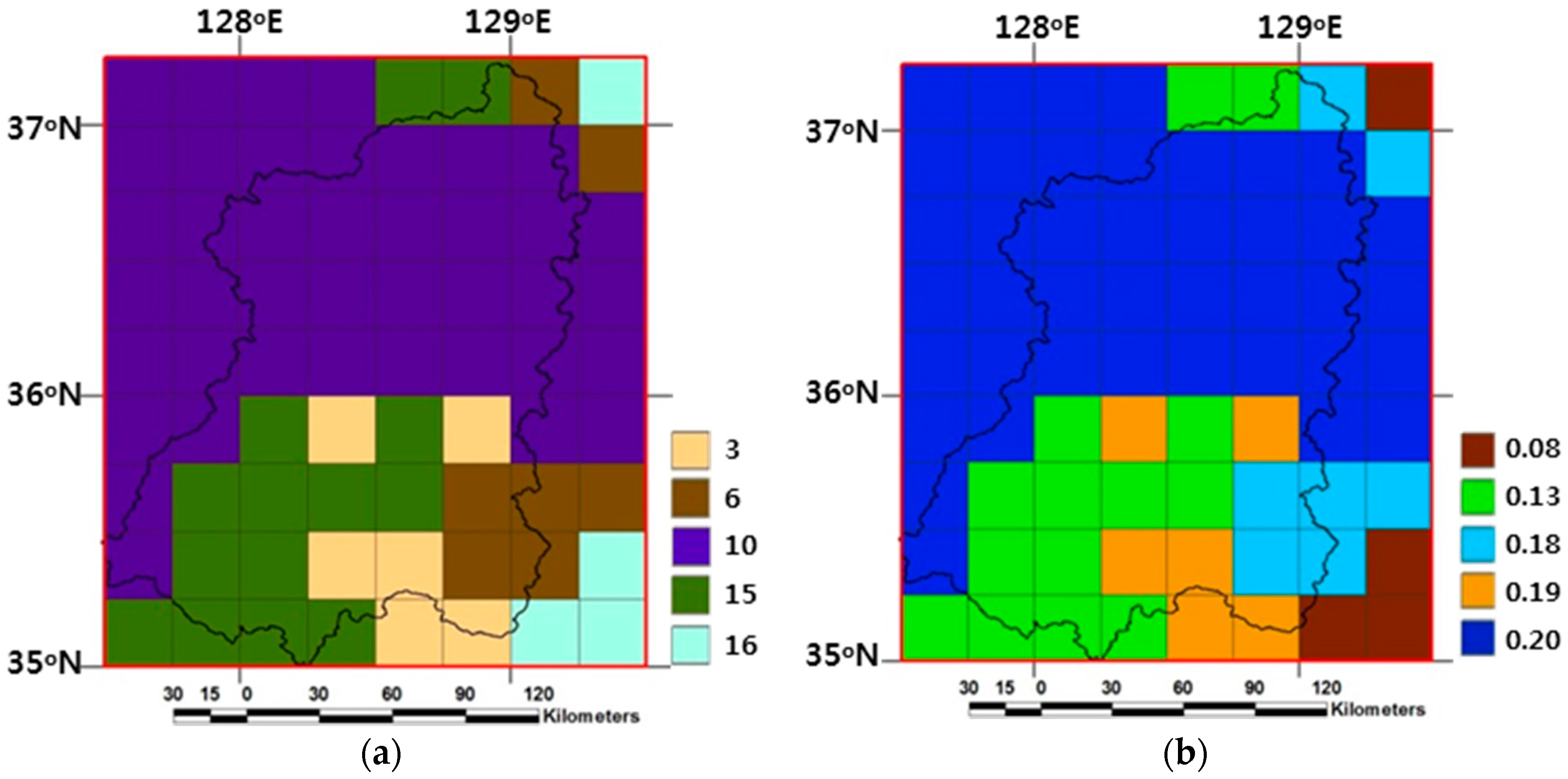
The vegetative SBCs include land cover category, albedo, fractional vegetation cover, and monthly leaf area index in 2009. First of all, the raw data at much finer than the 30-km resolution on various data format and map projections were converted into ArcGIS raster data, and then the representative (majority or average) values were computed for each 30-km computational grid. The 30-km land cover category data was made from the 1-km USGS land cover classification with 24 categories [36], developed from the Advanced Very High Resolution Radiometer (AVHRR) satellite-derived Normalized Difference Vegetation Index (NDVI) composites. The one of the USGS 24 land cover types constituting the largest fraction is selected as the representative value for each 30-km grid. Provided that category 16 (water bodies) with the largest fraction is not the absolute majority in a grid, this grid’s land cover type is not the water body but belongs in the category that constitutes the second largest fraction. As shown in Figure 2a, the study watershed consists of the USGS land cover categories 3 (irrigated cropland and pasture), 6 (cropland/woodland mosaic), 10 (savanna), and 15 (mixed forest) at the 30-km scale. The three water body (category 16) grids in the study domain were used as the standard identification for consistency of water bodies in all datasets of SBCs. Following Yucel [37], the 30-km albedo values were assigned with respect to the 30-km USGS land cover categories, distributed from 0.13 to 0.20 for the study watershed and given to 0.08 for water bodies as shown in Figure 2b. The high-resolution fractional vegetation cover was computed following Zeng et al. [38,39] from the 1-km NDVI data in the Système Pour l’Observation de la Terre-VEGETATION (SPOT-VGT) satellite products [40]. Figure 2c denotes spatial distributions of the 30-km fractional vegetation cover values ranging from 83.2% to 100%, calculated by averaging all 1-km values within each 30-km grid using a zonal statistic function, ZONALMEAN in ArcGIS geoprocessing tools. The raw leaf area index data is provided from the 1-km MOD 15 LAI data [41] by Moderate Resolution Imaging Spectroradiometer (MODIS) from the Terra (EOS AM) and Aqua (EOS PM) satellites. After abnormal values were removed by a smoothing filter method by Liang et al. [16] and then missing values were filled using an interpolation method by Choi [29], the monthly leaf area index data were calculated following Zeng et al. [39] for each 30-km grid by the ZONEALMEAN function in ArcGIS. Figure 2d denotes leaf area index values in a range of 2.3 to 4.6 for the study domain in July 2009.

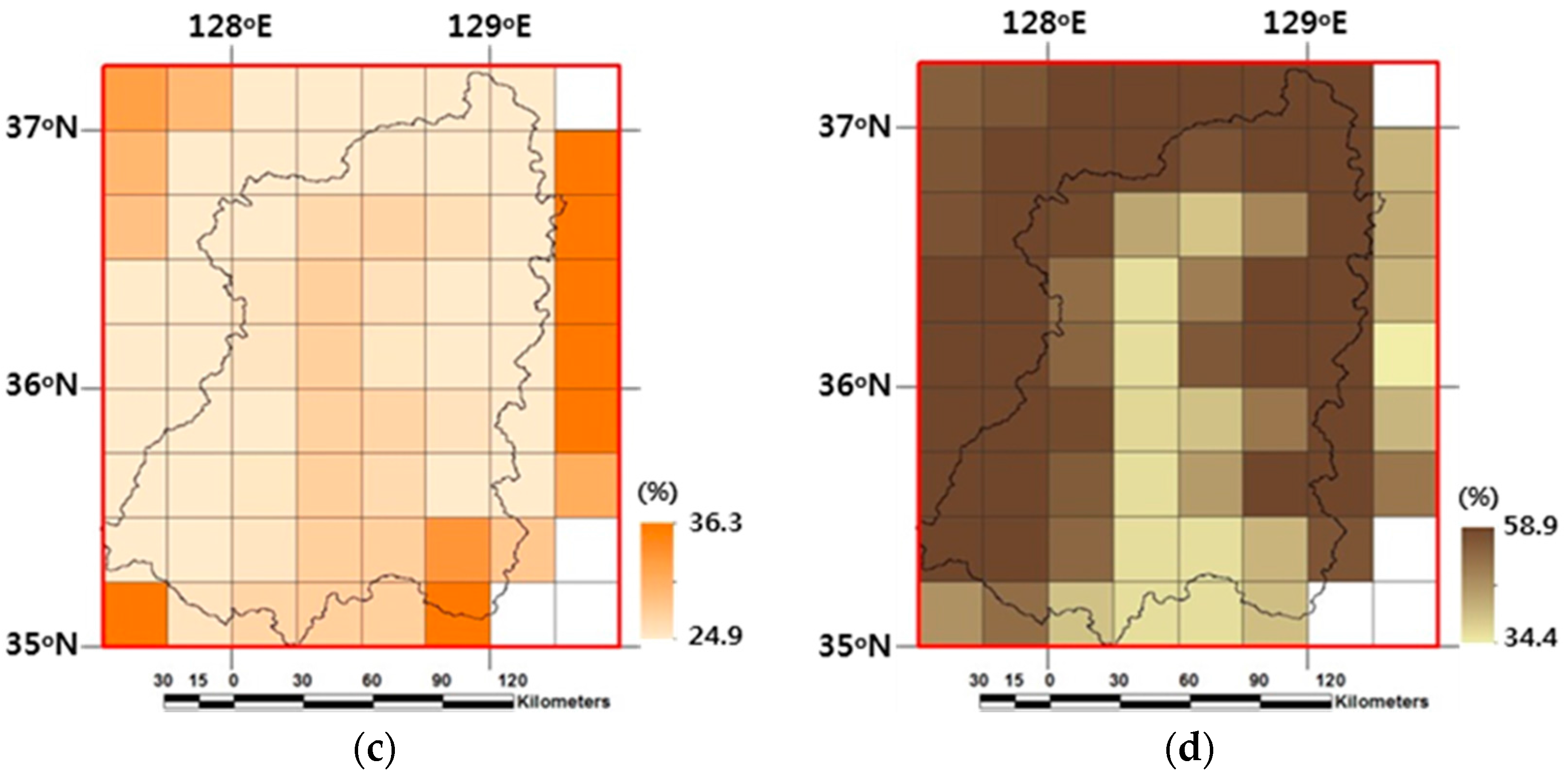
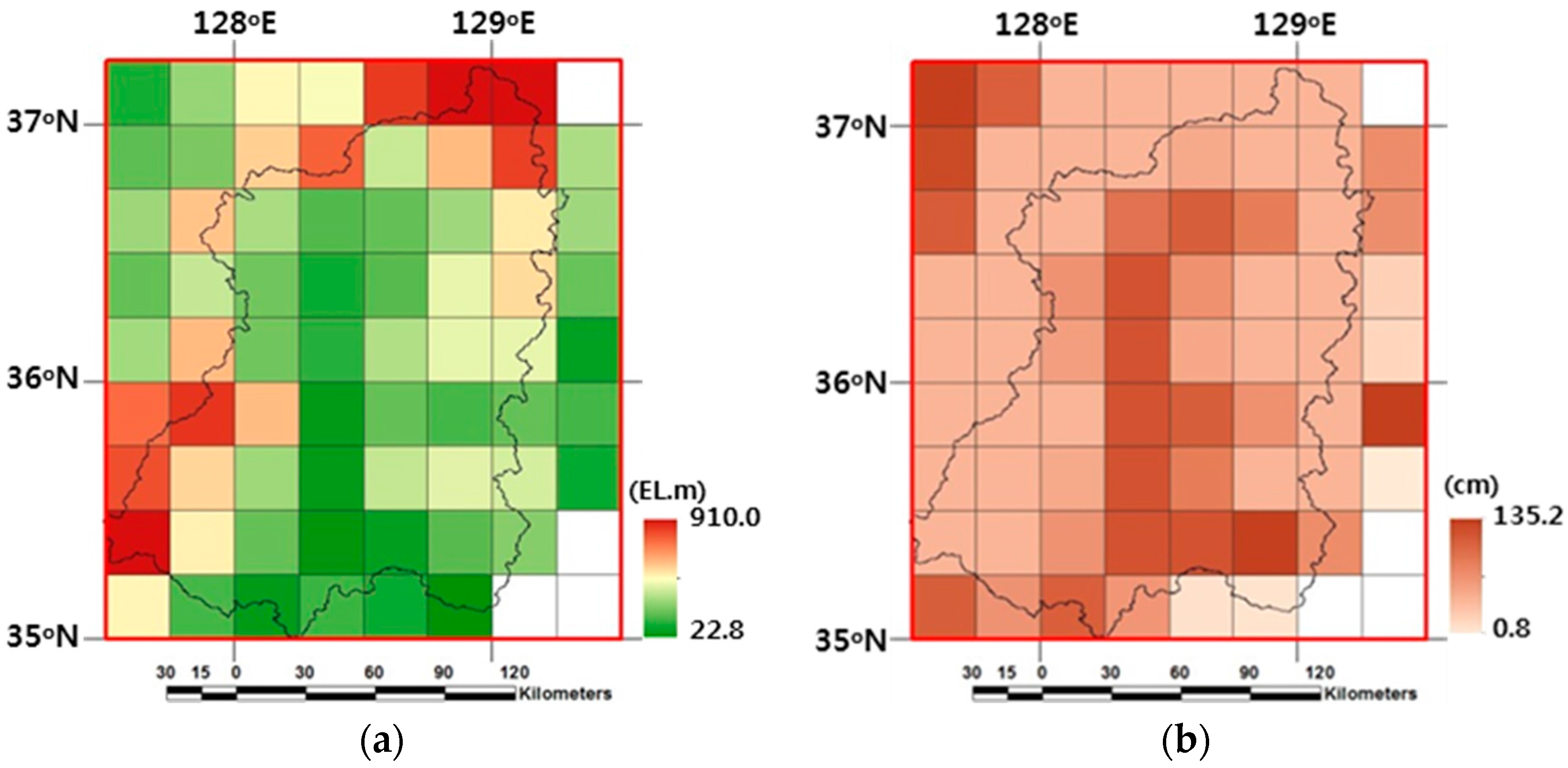
The terrain SBCs comprise surface elevation, bedrock depth, and soil sand/clay fraction profiles over the 11 soil layers at the 30-km resolution. After higher resolution raw data on various data formats and map projections were converted into ArcGIS raster data, the average of all raster values within each 30-km grid was calculated by the ZONALMEAN function in ArcGIS. The surface elevation data was constructed from the 90-m (3 arc-second) DEM provided by the National Aeronautics and Space Administration (NASA) Shuttle Radar Topographic Mission (SRTM) DEM dataset [42]. The 30-km surface elevation data ranges from 22.8 to 910.0 EL.m for the study domain as shown in Figure 3a. The bedrock depth and soil sand/clay fraction profiles were constructed by the Harmonized World Soil Database (HWSD) [43], developed by the Land Use Change (LUC) project of International Institute for Applied Systems Analysis (IIASA) and the Food and Agriculture Organization of the United Nations (FAO). The spatial distribution of the bedrock depth is in the range from 0.8 to 135.2 cm below the surface ground as shown in Figure 3b. Figure 3c,d denote the 30-km soil composition fraction results for the first soil model layer, ranging between 24.9% and 36.3% for sand, and between 34.4% and 58.9% for clay.

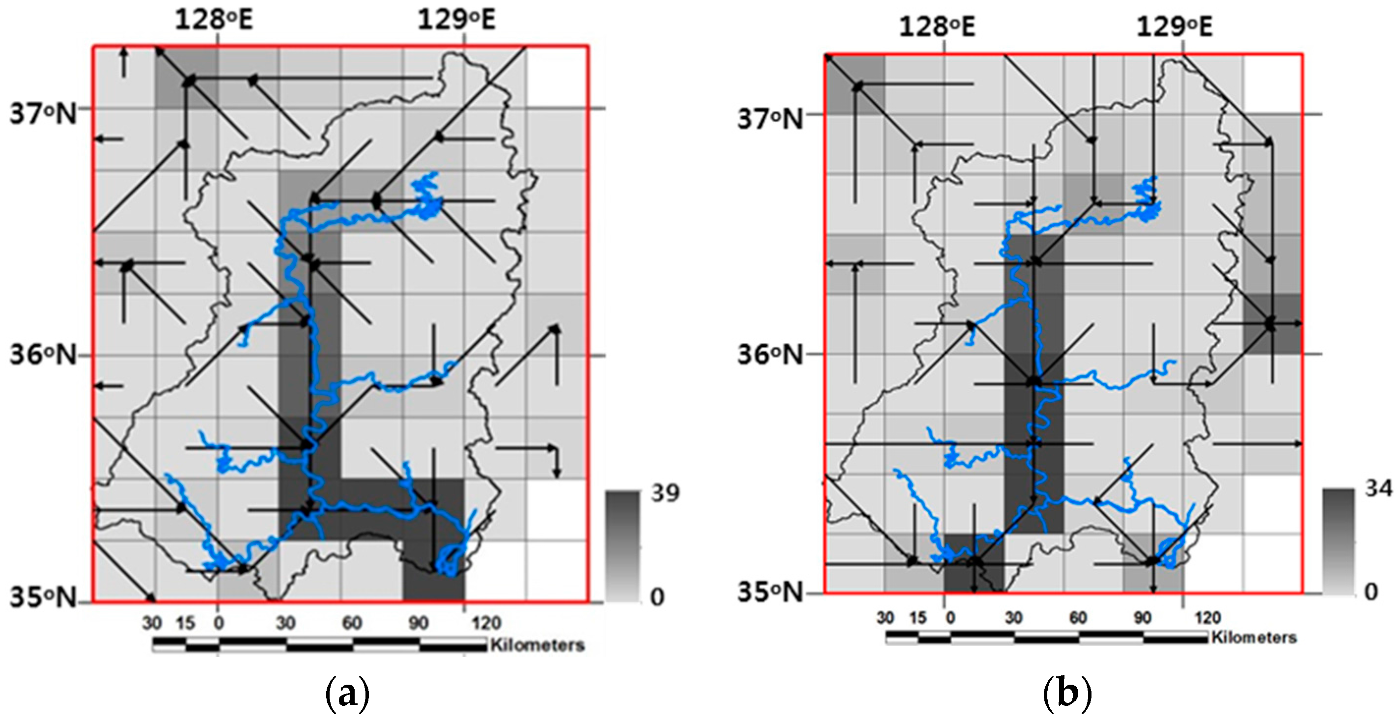
The new CoLM+LF requires additional SBCs on the lateral flow information such as flow direction and accumulation data for each 30-km grid to perform the topographically controlled surface and subsurface flow computations. These fields were constructed by our own upscaling method using the reference flow information data at finer resolution possible, the 90-m (3 arc-second) terrain and drainage data provided by the Hydrological data and maps based on SHuttle Elevation Derivatives at multiple Scales (HydroSHEDS) [44], derived from the NASA SRTM DEM. The HydroSHEDS geospatial dataset is known to provide the realistic stream flow direction data through a sequence of algorithms such as void-filling, filtering, hydrologic conditioning, stream burning, manual corrections, and upscaling techniques on the original SRTM DEM for improvements to data information accuracy suitable for hydrologic study applications. Figure 4 compares the difference between the 30-km flow information datasets derived from our own upscaling method using the 90-m HydroSHEDS data and from the eight direction flow model using the 30-km SBC of surface elevation in ArcGIS. The 30-km flow information result upscaled by our own method properly represents and is much closer to the main streamline of the Nakdong River in the study domain. The 30-km lateral flow SBCs have a significant influence on the lateral surface and subsurface flow computation as well as the drainage area delineation.

To prevent any inconsistency over all the 30-km SBCs due to different sources of the raw data, all constructed SBCs were adjusted by the 30-km land cover category as the standard identification for land and water body grids.

3.3. Meteorological Forcing Data

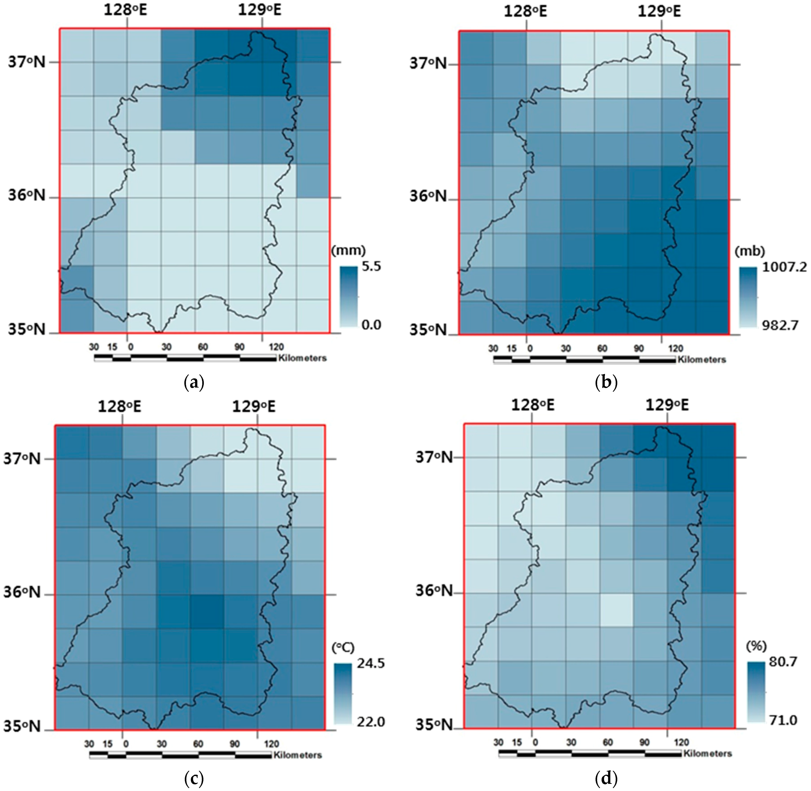
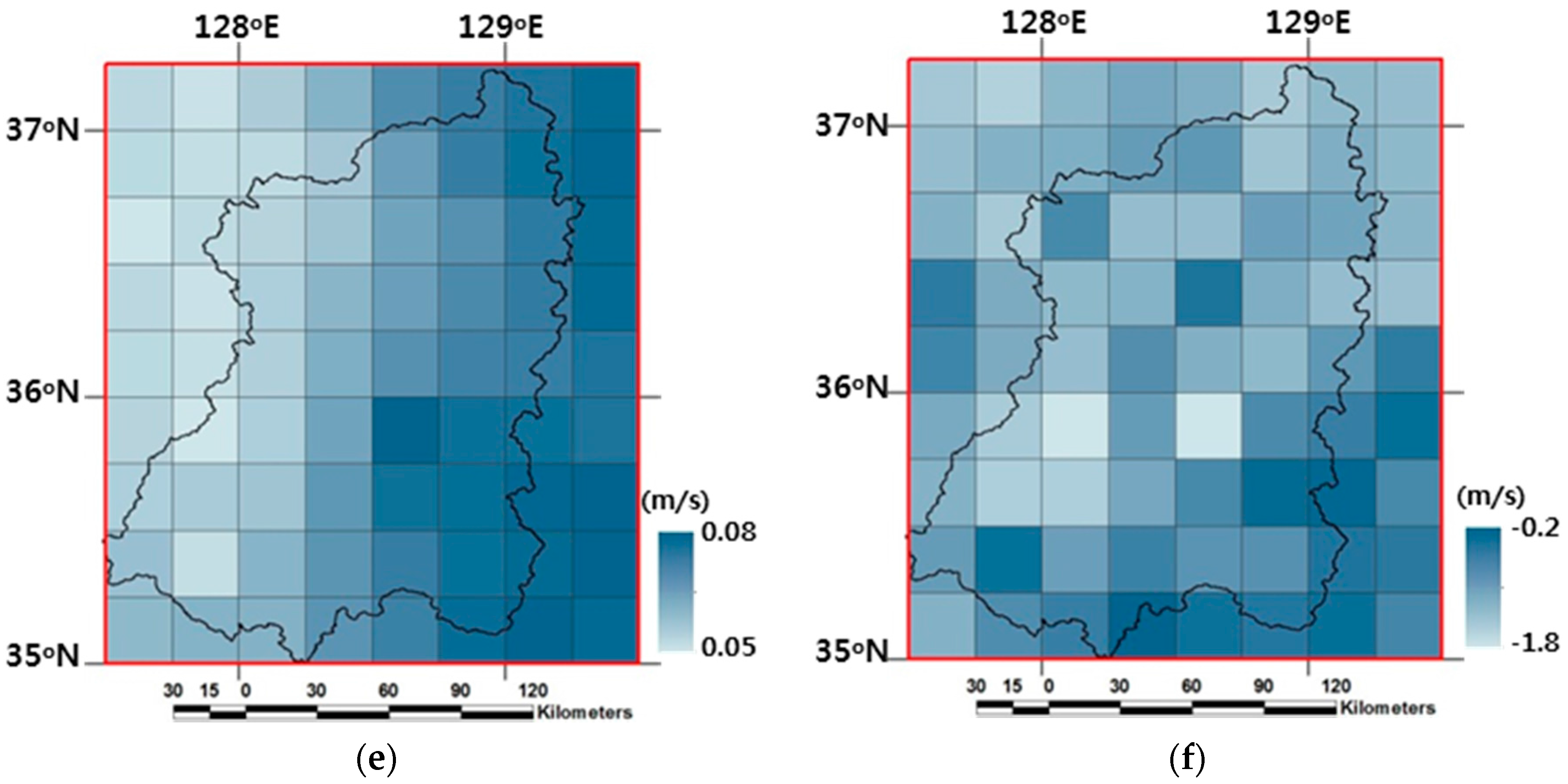
The meteorological forcing variables are required for both the CoLM and the CoLM+LF simulations in the offline mode. Most meteorological forcing data to drive both model simulations during the year of 2009 were also constructed onto the 30-km computational grids by the ZONALMEAN function in ArcGIS after in situ observations at 19 KMA meteorological gauge stations around the study watershed were spatially interpolated onto the study domain with average values weighted by the inverse of the distance from the gauge point. The 30-km daily meteorological forcing data constructed in this study are precipitation (mm), snow (cm), air pressure (hPa), vapor pressure (hPa), air temperature (°C), specific humidity (%), zonal and meridional wind speeds (m/s), and downward short wave radiation (MJ/m²). The daily meteorological forcing data were linearly interpolated for the computational time step of 600 seconds in the both models.

Figure 5 denote spatial distributions of selective meteorological forcing data for the study domain on 5 July, one day of precipitation events in 2009.

3.4. Initial Conditions

To resolve uncertainty in the initial conditions, both CoLM and CoLM+LF under the assumed initial conditions on 1 January 2009 were run six times repeatedly without interruption for the whole of 2009. The sixth set of results from CoLM and CoLM+LF was saved for analysis and interpretation.

4. Results

The runoff results simulated from both CoLM and CoLM+LF at the 30-km resolution were compared with streamflow discharges observed at the Jindong gauge station by the MOLIT around the outlet of the study watershed. For the performance assessment of both model simulations, the relative agreement of the model results with the observations was evaluated by the Nash–Sutcliffe efficiency (NSE) [45] and the absolute value of the relative bias (ARB), a set for assessing the goodness of fit as suggested by McCuen et al. [46] as:

$$NSE=1-\frac{{\displaystyle \sum _{i=1}^n{(O_i-S_i)}^2}}{{\displaystyle \sum _{i=1}^n{(O_i-\overline{O})}^2}},$$

(13)

$$ARB=\frac{\left|{\displaystyle \sum _{i=1}^n(O_i-S_i)}\right|}{\overline{O}},$$

(14)

where $n$ is total number of data, $O_i$ is the observed data and $S_i$ is the simulated data at day $i$, and $\overline{O}$ is the average of $O_i$. NSE can assess the model predictive ability and ARB is used to compute total volume error in model predictions.

4.1. Runoff Results from the Baseline CoLM

Total runoff is comprised of surface and subsurface runoff parts. Since total runoff for a watershed was calculated by the sum of watershed-wide averages of surface runoff and subsurface runoff in the baseline CoLM simulations, total runoff was calculated from average values over all upstream grid cells of the target grid with the Jindong gauge station. Total runoff simulation results were compared with daily specific discharges (discharge per unit drainage area) observed at the Jindong stream gauge station in the study watershed during the year of 2009. Following Choi and Liang [9], the sensitivity of the baseline CoLM was examined to two calibration parameters, the hydraulic conductivity decay factor f and the maximum baseflow coefficient $R_{sb,\max }$ for runoff simulations in the Nakdong River Watershed.

Figure 6 denotes both NSE and ARB scores for runoff results under a set of two calibration parameters in a wide range from 2 to 9 m⁻¹ for the hydraulic conductivity decay factor f and from 1 × 10⁻⁵ to 9 × 10⁻¹ mm/s for the maximum baseflow coefficient $R_{sb,\max }$. NSE scores are low and negative on the whole analysis, and the maximum score of −0.140 occurs with a tolerable ARB of 0.367 when the hydraulic conductivity decay factor f is 7 m⁻¹ and the maximum baseflow coefficient $R_{sb,\max }$ is 7 × 10⁻¹ mm/s. These two calibration parameters play a significant role in the baseflow generation for the baseline CoLM without the topographically controlled lateral flow scheme.

4.2. Runoff Results from the New CoLM+LF

In the CoLM+LF that can simulate surface outflow at each grid, total runoff was calculated by the sum of the specific discharge of surface flow and the upstream grid-averaged subsurface runoff for a target grid point as:

$$R_{tot}=\frac{Q_s}{(n_{fa}+1)A}+{\overline{R}}_{sb}$$

(15)

where $R_{tot}$ is total runoff, $n_{fa}$ is the flow accumulation number at the target grid point, and ${\overline{R}}_{sb}$ is the averaged subsurface runoff for the total grid cells located upstream of the target grid point.

The CoLM+LF runoff simulations were examined to two calibration parameters, the hydraulic conductivity decay factor $f$ values from 2 to 9 m⁻¹ and the hydraulic conductivity anisotropic ratio $\zeta$ values from 10 to 10⁶. Figure 7 represents both NSE and ARB scores between total runoff results from the CoLM+LF and specific discharges observed at the Jindong stream gauge station for the study watershed in 2009. Overall, both NSE and ARB scores are much better than those for the baseline CoLM results, and the hydraulic conductivity decay factor $f$ of 3 m⁻¹ and the hydraulic conductivity anisotropic ratio $\zeta$ of 10⁴ are calibrated in considering synchronization performance results for NSE of 0.774 and ARB of 0.012.

4.3. Comparison of Runoff Results

Figure 8 compares the time series of daily specific discharges (total runoff) during 2009 simulated from the baseline CoLM and the new CoLM+LF under each calibrated parameter set, along with observations at the Jindong gauge station in the study watershed.

Table 1. Comparison of the model performance measured by the Nash–Sutcliffe coefficient, NSE and the absolute relative bias, ARB for daily runoff results in the study watershed during 2009 simulated from the baseline CoLM under the calibrated values of the hydraulic conductivity decay factor f and the maximum baseflow coefficient R_sb,max and from the new CoLM+LF under the calibrated values of the hydraulic conductivity decay factor f and the hydraulic conductivity anisotropic ratio $\zeta$.

Models	Model Performance		Calibration Parameters
	NSE	ARB	f	${\mathit{R}}_{\mathit{s}\mathit{b},\mathbf{max}}$ or $\mathit{\zeta }$
CoLM	−0.140	0.367	7 m−1	7 × 10−1 mm/s
CoLM+LF	0.774	0.012	3 m−1	104

summarizes model performance results measured by NSE = −0.140 and ARB = 0.367 for the baseline CoLM under calibrated parameters of f = 7 m⁻¹ and $R_{sb,\max }$ = 7 × 10⁻¹ mm/s, and NSE = 0.774 and ARB = 0.012 for the new CoLM+LF under calibrated parameters of f = 3 m⁻¹ and $\zeta$ = 10⁴, respectively. As shown in Figure 8 and Table 1, the seasonal variability of observed streamflow is realistically captured by the runoff result from the CoLM+LF incorporating the lateral surface and subsurface flow schemes, whereas the baseline CoLM generates high peak discharges due to immediate response to precipitation events without surface flow routing or runoff travel time effect over the watershed, leading to the overestimated runoff result in total volume. Moreover, the runoff result from the baseline CoLM without considering impacts of surface flow depth on the infiltration rate may make errors in both infiltration and surface flow calculations. The new CoLM+LF scheme significantly improves the performance of the baseline CoLM simulation in representing the watershed runoff prediction.

Figure 9 compares surface runoff and subsurface runoff components separately from both the baseline CoLM and the new CoLM+LF simulations under each calibrated parameter set. The baseline CoLM simulates surface runoff with much higher and shaper peaks than the new CoLM+LF result. Although the baseline CoLM simulation generates much enhanced baseflow by larger values of the two calibration parameters to capture the recession parts in the observed hydrograph, even the selected set of two calibration parameters still generates unrealistic high peaks due to quick response of surface runoff to precipitation events in the baseline CoLM. On the contrary, the lateral surface and subsurface flow computations play an important part in capturing the seasonal streamflow patterns in the new CoLM+LF result. The CoLM+LF incorporating the lateral surface flow scheme generates lower peaks and declining recession curves in surface runoff by the surface flow routing effect, and the baseflow is effectually generated by the surface flow depth contribution to infiltration with a lower $f$ value than the baseline CoLM simulation. It is found that the watershed runoff is much more realistically predicted in the new CoLM+LF parameterizations by interactions between the lateral surface flow and the subsurface flow controlled by topography.

5. Discussion

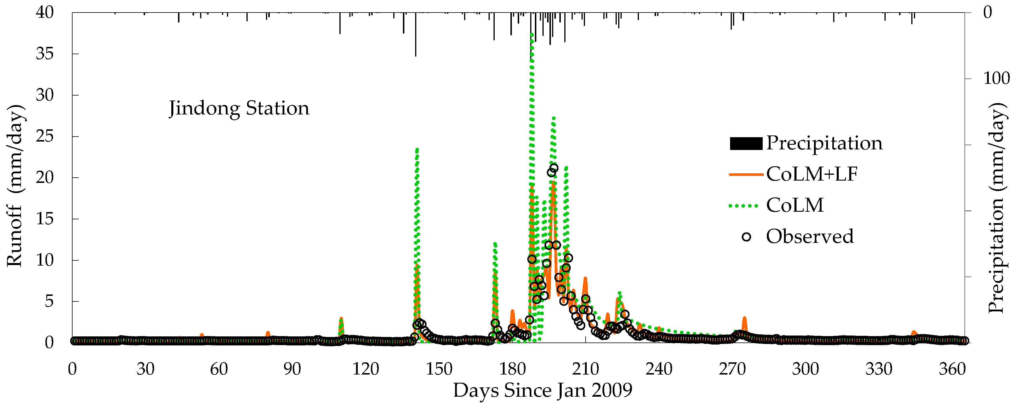
Like most existing LSMs, the baseline CoLM predicts runoff from local net excess water flux after excluding surface evapotranspiration and soil moisture flux from precipitation. A disregard for the role of lateral surface and subsurface runoff in the terrestrial hydrologic cycle may make significant errors in the baseline CoLM simulations. This study has therefore introduced a new model, the CoLM+LF that incorporates the 1D diffusion wave surface flow model and the 1D topographically controlled baseflow scheme into the existing formulations for the terrestrial hydrologic cycle in the baseline CoLM. The baseline CoLM and the new CoLM+LF were implemented for the Nakdong River Watershed in Korea in a standalone mode by the realistic SBCs and meteorological forcings on the 30-km grid mesh for mesoscale applications by direct interactions between hydrological and atmospheric components. This study has collected high quality observational data mainly by multispectral remote sensing products and in situ observations from finer possible spatial data. The various raw data were spatially transformed into the proper representative values on the 30-km spacing grids in the study domain by our own program codes and geoprocessing tools in ArcGIS. The new CoLM+LF simulations need the additional SBCs such as the 30-km flow direction and accumulation data to implement an explicit lateral flow scheme. Since it is problematic to directly use the eight direction flow model provided by ArcGIS on the 30-km resolution grids, our own upscaling method properly generated the 30-km flow direction result, which coincides better with the Nakdong River stream network, compared with the result from ArcGIS. This study has successfully provided a primary set of SBCs and daily meteorological forcing data during the year 2009 for the study domain, including the entire Nakdong River Watershed from the comprehensive Earth observations.

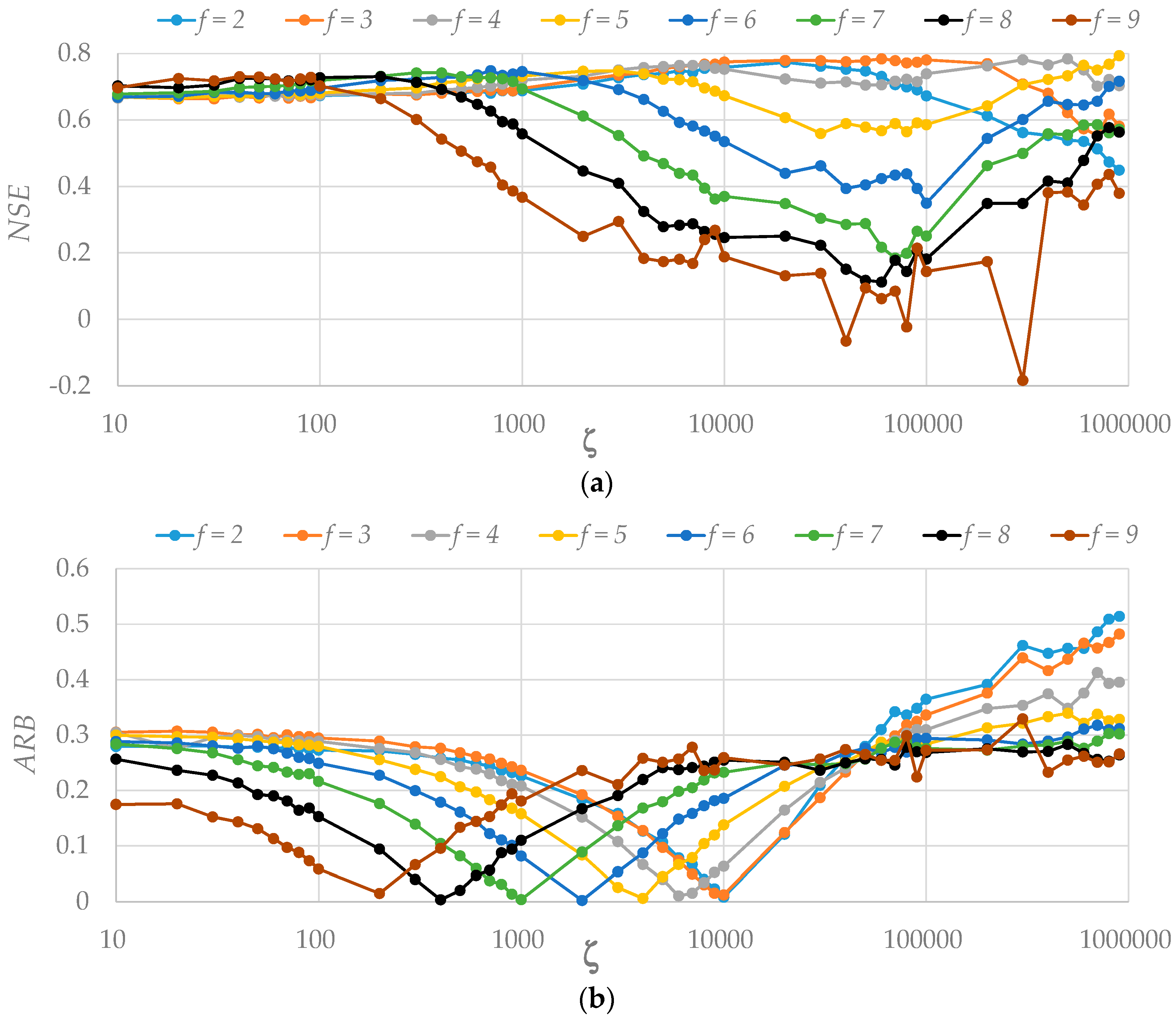
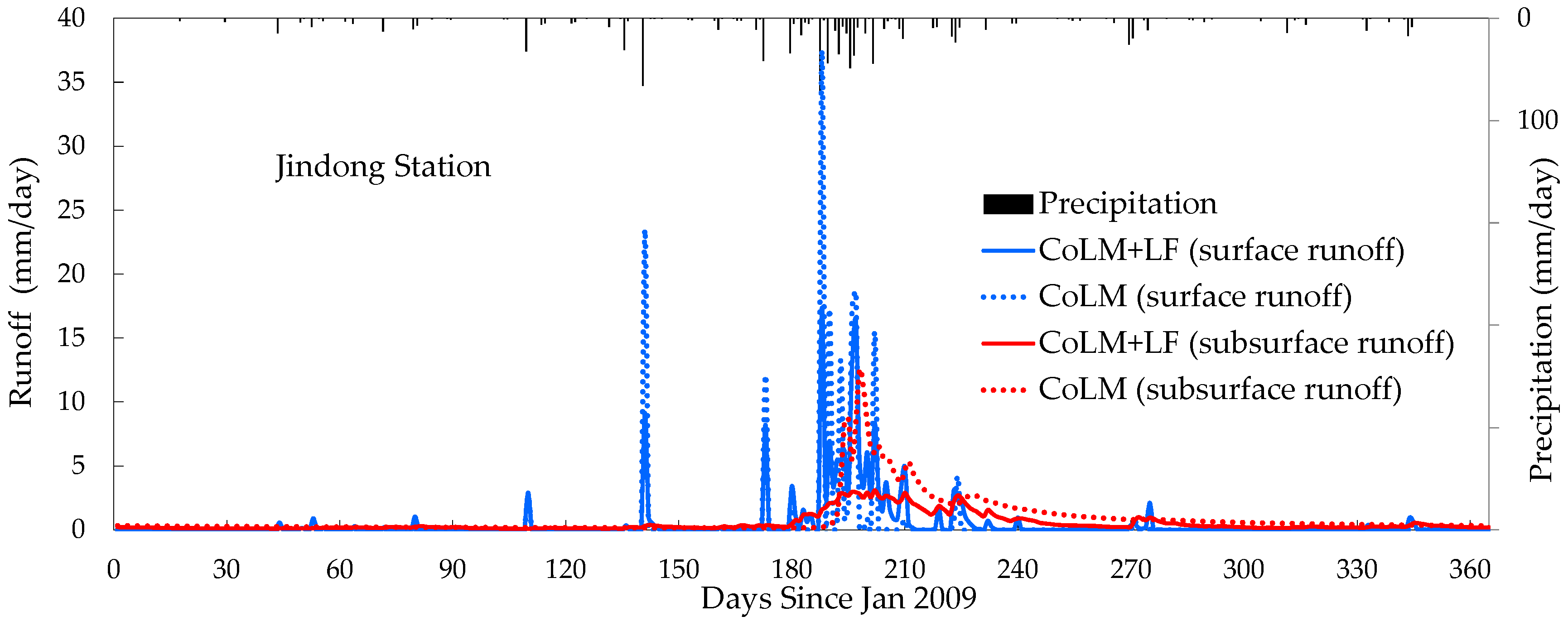
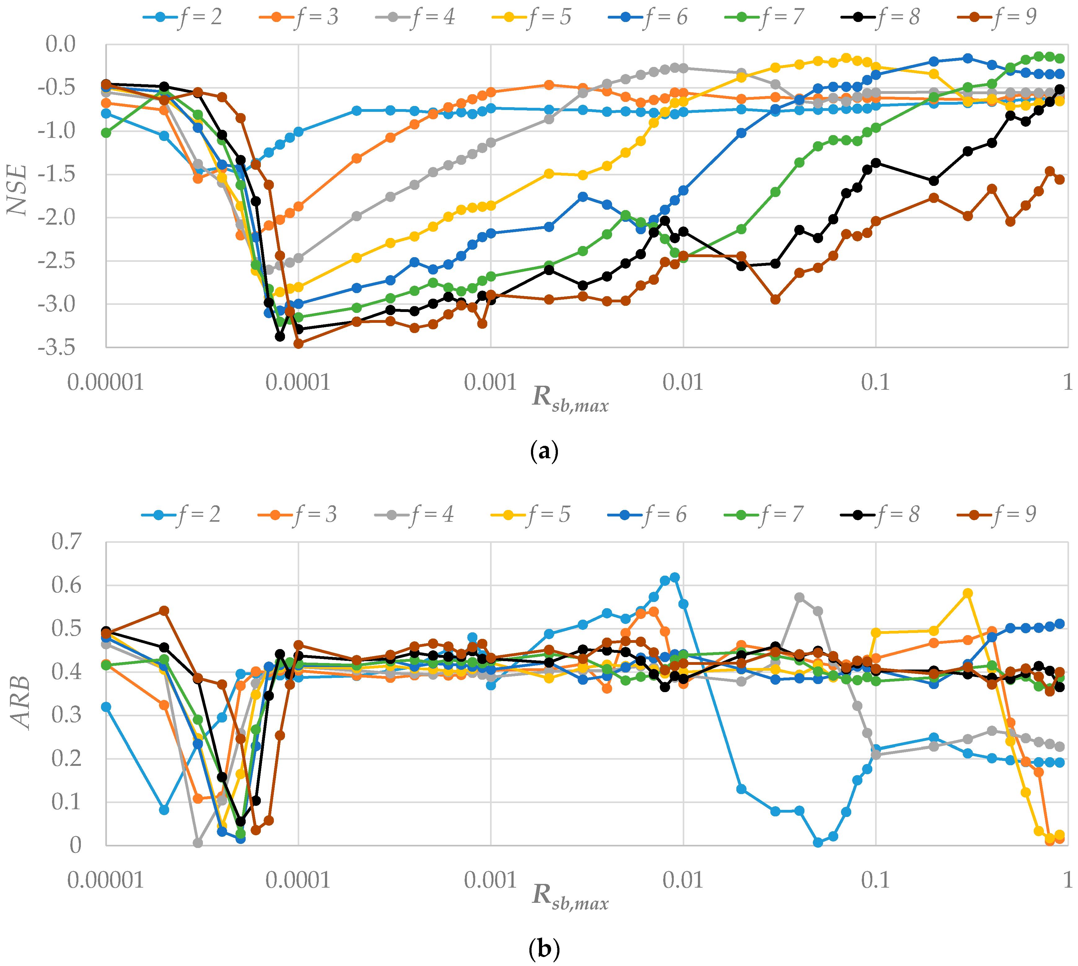
This study has evaluated the performance of the CoLM and the CoLM+LF in offline simulations of daily runoff through the sensitivity analysis of key parameters for runoff variables at a watershed scale by comparison of the simulated results with observations at the Jindong gauge station in the study watershed. Surface runoff generated simply from the local net excess water in each grid disappears at the next computational time step in the baseline CoLM. Since surface runoff calculated at every time step irrespective of the remaining surface runoff at the previous time step makes no contribution to infiltration, larger values of the two calibration parameters (decay factor f and the maximum baseflow coefficient $R_{sb,\max }$) were estimated for the baseline CoLM to enhance both infiltration and baseflow generation. As the baseflow equation in the baseline CoLM is apt to underestimate baseflow, as demonstrated in Choi and Liang [9], runoff recession curves observed at the Jindong gauge station cannot be captured by runoff results generated with $R_{sb,\max }$ values in the order of 10⁻⁴ mm/s used in previous studies [6,7,9,25]. Accordingly, the baseline CoLM simulations that predict sharp and steep peaks in surface runoff were tuned by larger values for f of 7 m⁻¹ and $R_{sb,\max }$ of 7 × 10⁻¹ mm/s to enhance baseflow generation. Such simplistic assumptions and crude parameterizations for the lateral surface and subsurface runoff processes in the baseline CoLM may cause significant model errors and consequently unrealistic model parameters by calibration. On the other hand, the new CoLM+LF incorporating an explicit surface flow routing scheme can facilitate infiltration by the surface flow depth contribution, leading to the enhanced baseflow generation as well. Moreover, baseflow can be effectually generated in the new CoLM+LF by a new formulation for baseflow controlled by topography which can also depict the effects of surface macropores and vertical hydraulic conductivity changes. In the new CoLM+LF with a set of the lateral surface and subsurface runoff schemes, lower peaks and smoother recession curves of surface runoff were generated under relatively smaller value for f of 3 m⁻¹ due to the surface flow routing effect, and the baseflow were successfully generated by the surface flow depth contribution to infiltration and topographically controlled baseflow scheme with the hydraulic conductivity anisotropic ratio $\zeta$ of 10⁴.

This study has demonstrated that the CoLM+LF incorporating the topographically controlled surface and subsurface flow computations realistically can predict the temporal variation of the spatial distribution of streamflow runoff at a watershed scale, while the baseline CoLM may generate unrealistic surface runoff and infiltration results, which are important components for terrestrial water distribution and movement. The new CoLM+LF provides improved runoff modeling capability to the baseline CoLM for better streamflow predictions affecting the terrestrial hydrologic cycle crucial to climate variability and change studies. The new CoLM+LF is expected to be a helpful and essential tool for water resource management and hydrological impact assessment, particularly in regions with complex topography. This proposed CoLM+LF targeted for mesoscale climate application and watershed scale hydrologic analysis at relatively large spatial scales needs to be implemented for comprehensive terrestrial hydrologic simulations with long-term observations after climatological data are constructed over various watersheds including this study domain. The next study is planning to perform an analysis on uncertainties in the SBCs constructed from various remote sensing products and examine the sensitivity of model predictability to the spatial and temporal resolutions of input data. The next model also needs to include aquifer recharge, deep aquifer groundwater, channel flow routing, and regulation storage for further investigation.

References

1. Sellers, P.J.; Los, S.O.; Tucker, C.J.; Justice, C.O.; Dazlich, D.A.; Collatz, G.J.; Randall, D.A. A revised land surface parameterization (SiB2) for atmospheric GCMs. Part II: The generation of global fields of terrestrial biophysical parameters from satellite data. J. Clim. 1996, 9, 706–737. [Google Scholar] [CrossRef]
2. Bates, B.C.; Kundzewicz, Z.W.; Wu, S.; Palutikof, J.P. Climate Change and Water; Technical Paper of Intergovernmental Panel on Climate Change; IPCC Secretariat: Geneva, Switzerland, 2008; p. 210. [Google Scholar]
3. Stieglitz, M.; Rind, D.; Famiglietti, J.; Rosenzweig, C. An efficient approach to modeling the topographic control of surface hydrology for regional modeling. J. Clim. 1997, 10, 118–137. [Google Scholar] [CrossRef]
4. Chen, J.; Kumar, P. Topographic influence of the seasonal and interannual variation of water and energy balance of basins in North America. J. Clim. 2001, 14, 1989–2014. [Google Scholar] [CrossRef]
5. Warrach, K.; Stieglitz, M.; Mengelkamp, H.T.; Raschke, E. Advantages of a topographically controlled runoff simulation in a soil-vegetation-atmosphere transfer model. J. Hydrometeorol. 2002, 3, 131–148. [Google Scholar] [CrossRef]
6. Niu, G.Y.; Yang, Z.L. The versatile integrator of surface and atmosphere processes (VISA) Part II: Evaluation of three topography based runoff schemes. Glob. Planet. Chang. 2003, 38, 191–208. [Google Scholar] [CrossRef]
7. Niu, G.Y.; Yang, Z.L.; Dickinson, R.E.; Gulden, L.E. A simple TOPMODEL-based runoff parameterization (SIMTOP) for use in GCMs. J. Geophys. Res. 2005, 110. [Google Scholar] [CrossRef]
8. Oleson, K.W.; Niu, G.Y.; Yang, Z.L.; Lawrence, D.M.; Thornton, P.E.; Lawrence, P.J.; Stockli, R.; Dickinson, R.E.; Bonan, G.B.; Levis, S.; et al. Improvements to the community land model and their impact on the hydrological cycle. J. Geophys. Res. 2008, 113. [Google Scholar] [CrossRef]
9. Choi, H.I.; Liang, X.Z. Improved terrestrial hydrologic representation in mesoscale land surface models. J. Hydrometeorol. 2010, 11, 797–809. [Google Scholar] [CrossRef]
10. Choi, H.I.; Liang, X.Z.; Kumar, P. A conjunctive surface–Subsurface flow representation for mesoscale land surface models. J. Hydrometeorol. 2013, 14, 1421–1442. [Google Scholar] [CrossRef]
11. Schmid, B.H. On overland flow modelling: Can rainfall excess be treated as independent of flow depth? J. Hydrol. 1989, 107, 1–8. [Google Scholar] [CrossRef]
12. Wallach, R.; Grigorin, G.; Rivlin, J. The errors in surface runoff prediction by neglecting the relationship between infiltration rate and overland flow depth. J. Hydrol. 1997, 200, 243–259. [Google Scholar] [CrossRef]
13. Singh, V.; Bhallamudi, S.M. A complete hydrodynamic border-strip irrigation model. J. Irrig. Drain. Eng. 1997, 122, 189–197. [Google Scholar] [CrossRef]
14. Dai, Y.; Zeng, X.; Dickinson, R.E.; Baker, I.; Bonan, G.B.; Bosilovich, M.G.; Denning, A.S.; Dirmeyer, P.A.; Houser, P.R.; Niu, G.; et al. The common land model. Bull. Am. Meteorol. Soc. 2003, 84, 1013–1023. [Google Scholar] [CrossRef]
15. Liang, X.Z.; Choi, H.I.; Kunkel, K.E.; Dai, Y.; Joseph, E.; Wang, J.X.L.; Kumar, P. Development of the Regional Climate-Weather Research and Forecasting Model (CWRF): Surface Boundary Conditions; ISWS SR 2005-01; Illinois State Water Survey: Champaign, IL, USA, 2005; p. 32. [Google Scholar]
16. Liang, X.Z.; Choi, H.I.; Kunkel, K.E.; Dai, Y.; Joseph, E.; Wang, J.X.L.; Kumar, P. Surface boundary conditions for mesoscale regional climate models. Earth Interact. 2005, 9, 1–28. [Google Scholar] [CrossRef]
17. Liang, X.Z.; Xu, M.; Gao, W.; Kunkel, K.E.; Slusser, J.; Dai, Y.; Min, Q.; Houser, P.R.; Rodell, M.; Schaaf, C.B.; et al. Development of land surface albedo parameterization bases on Moderate Resolution Imaging Spectroradiometer (MODIS) data. J. Geophys. Res. 2005, 110. [Google Scholar] [CrossRef]
18. Liang, X.Z.; Xu, M.; Zhu, J.; Kunkel, K.E.; Wang, J.X.L. Development of the regional climate-weather research and forecasting model (CWRF): Treatment of topography. In Proceedings of the 2005 WRF/MM5 User’s Workshop, Boulder, CO, USA, 27–30 June 2005; p. 5.
19. Liang, X.Z.; Xu, M.; Choi, H.I.; Kunkel, K.E.; Rontu, L.; Geleyn, J.F.; Müller, M.D.; Joseph, E.; Wang, J.X.L. Development of the regional Climate-Weather Research and Forecasting model (CWRF): Treatment of subgrid topography effects. In Proceedings of the 7th Annual WRF User’s Workshop, Boulder, CO, USA, 19–22 June 2006; p. 5.
20. Choi, H.I. 3-D Volume Averaged Soil-Moisture Transport Model: A Scalable Scheme for Representing Subgrid Topographic Control in Land-Atmosphere Interactions. Ph.D. Dissertation, University of Illinois at Urbana-Champaign, Champaign, IL, USA, 2006; p. 189. [Google Scholar]
21. Choi, H.I.; Kumar, P.; Liang, X.Z. Three-dimensional volume-averaged soil moisture transport model with a scalable parameterization of subgrid topographic variability. Water Resour. Res. 2007, 43, W04414. [Google Scholar] [CrossRef]
22. Liang, X.Z.; Xu, M.; Yuan, X.; Ling, T.; Choi, H.I.; Zhang, F.; Chen, L.; Liu, S.; Su, S.; Qiao, F.; et al. Regional Climate-Weather Research and Forecasting Model (CWRF). Bull. Am. Meteorol. Soc. 2012, 93, 1363–1387. [Google Scholar] [CrossRef]
23. Liang, X.Z.; Chen, L.; He, Y.; Gan, Y. Evaluation of CWRF performance in simulating US climate variations. In Proceedings of the 2013 Fall Meeting, AGU, San Francisco, CA, USA, 9–13 December 2013.
24. Qian, T.; Dai, A.; Trenberth, K.E.; Oleson, K.W. Simulation of global land surface conditions from 1948 to 2004: Part I: Forcing data and evaluations. J. Hydrometeorol. 2006, 7, 953–975. [Google Scholar] [CrossRef]
25. Niu, G.Y.; Yang, Z.L. Effects of frozen soil on snowmelt runoff and soil water storage at a continental scale. J. Hydrometeor. 2006, 7, 937–952. [Google Scholar] [CrossRef]
26. Niu, G.Y.; Yang, Z.L.; Dickinson, R.E.; Gulden, L.E.; Su, H. Development of a simple groundwater model for use in climate models and evaluation with gravity recovery and climate experiment data. J. Geophys. Res. 2007, 112, D07103. [Google Scholar] [CrossRef]
27. Lawrence, P.J.; Chase, T.N. Representing a new MODIS consistent land surface in the Community Land Model (CLM3.0). J. Geophys. Res. 2007, 112, G01023. [Google Scholar] [CrossRef]
28. Lawrence, D.M.; Thornton, P.E.; Oleson, K.W.; Bonan, G.B. The partitioning of evapotranspiration into transpiration, soil evaporation, and canopy evaporation in a GCM: Impacts on land-atmosphere interaction. J. Hydrometeorol. 2007, 8, 862–880. [Google Scholar] [CrossRef]
29. Choi, H.I. Parameterization of high resolution vegetation characteristics using remote sensing products for the Nakdong River Watershed, Korea. Remote Sens. 2013, 5, 473–490. [Google Scholar] [CrossRef]
30. Choi, H.I. Application of a Land Surface Model Using Remote Sensing Data for High Resolution Simulations of Terrestrial Processes. Remote Sens. 2013, 5, 6838–6856. [Google Scholar] [CrossRef]
31. Horton, R.E. The Role of Infiltration in the Hydrologic Cycle. Eos Trans. Am. Geophys. Union 1933, 14, 446–460. [Google Scholar] [CrossRef]
32. Dunne, T.; Black, R.G. An Experimental Investigation of Runoff Production in Permeable Soils. Water Resour. Res. 1970, 6, 478–490. [Google Scholar] [CrossRef]
33. Sivapalan, M.; Beven, K.J.; Wood, E.F. On hydrologic similarity: 2. A scaled model of storm runoff production. Water Resour. Res. 1987, 23, 2266–2278. [Google Scholar] [CrossRef]
34. Beven, K.J.; Kirkby, M.J. A physically based, variable contributing area model of basin hydrology. Hydrol. Sci. Bull. 1979, 24, 43–69. [Google Scholar] [CrossRef]
35. Kumar, P.; Verdin, K.L.; Greenlee, S.K. Basin level statistical properties of topographic index for North America. Adv. Water Resour. 2000, 23, 571–578. [Google Scholar] [CrossRef]
36. The USGS Land Cover Institute (LCI). Available online: http://landcover.usgs.gov/landcoverdata.php (accessed on 30 December 2016).
37. Yucel, I. Effects of implementing MODIS land cover and albedo in MM5 at two contrasting US regions. J. Hydrometeorol. 2006, 7, 1043–1060. [Google Scholar] [CrossRef]
38. Zeng, X.; Dickinson, R.E.; Walker, A.; Shaikh, M.; DeFries, R.S.; Qi, J. Derivation and evaluation of global 1–km fractional vegetation cover data for land modeling. J. Appl. Meteorol. 2000, 39, 826–839. [Google Scholar] [CrossRef]
39. Zeng, X.; Shaikh, M.; Dai, Y.; Dickinson, R.E.; Myneni, R. Coupling of the common land model to the NCAR community climate model. J. Clim. 2002, 15, 1832–1854. [Google Scholar] [CrossRef]
40. SPOT-VEGETATION PROGRAMME. Available online: http://www.vgt.vito.be/ (accessed on 30 December 2016).
41. MOD 15—Leaf Are Index (LAI) and Fractional Photosynthetically Active Radiation (FPAR). Available online: http://cybele.bu.edu/download/manuscripts/mod15.pdf (accessed on 30 December 2016).
42. SRTM 90m Digital Elevation Database v4.1. Available online: http://www.cgiar-csi.org/data/srtm-90m-digital-elevation-database-v4-1 (accessed on 30 December 2016).
43. Harmonized World Soil Database v 1.2. Available online: http://webarchive.iiasa.ac.at/Research/LUC/External-World-soil-database/HTML/ (accessed on 30 December 2016).
44. (Hydrological data and maps based on SHuttle Elevation Derivatives at multiple Scales) HydroSHEDS. Available online: http://hydrosheds.cr.usgs.gov/index.php (accessed on 30 December 2016).
45. Nash, J.E.; Sutcliffe, J.V. River flow forecasting through conceptual models part I—A discussion of principles. J. Hydrol. 1970, 10, 282–290. [Google Scholar] [CrossRef]
46. McCuen, R.H.; Knight, Z.; Cutter, A.G. Evaluation of the Nash-Sutcliffe efficiency index. J. Hydrol. Eng. 2006, 11, 597–602. [Google Scholar] [CrossRef]
Figure 1. Location map for meteorological and stream gauge stations in the study watershed overlaid with the main streamline and the watershed boundary of the Nakdong River in Korea on the 30-km computational grid mesh.
Water 09 00148 g001
Figure 2. Spatial distributions of vegetative surface boundary conditions for (a) land cover category (3: irrigated cropland and pasture, 6: cropland/woodland mosaic, 10: savanna, 15: mixed forest, and 16: water bodies); (b) albedo; (c) fractional vegetation cover; and (d) July’s leaf area index on 30-km computational grids over the study domain.
Water 09 00148 g002aWater 09 00148 g002b
Figure 3. Spatial distributions of terrain surface boundary conditions for (a) surface elevation; (b) bedrock depth; (c) the first soil layer’s sand fraction; and (d) the first soil layer’s clay fraction on 30-km computational grids over the study domain.
Water 09 00148 g003aWater 09 00148 g003b
Figure 4. Comparison of lateral flow surface boundary conditions for the CoLM+LF flow direction (arrows) and flow accumulation (grey-black pixels) (a) from our own upscaling method; and (b) from ArcGIS eight direction method on 30-km computational grids with overlays of the main stream networks (blue lines) and the watershed boundary (black polygon) over the study domain.
Water 09 00148 g004
Figure 5. Spatial distributions of selective meteorological forcing variables for (a) precipitation; (b) air pressure; (c) air temperature; (d) specific humidity; (e) zonal wind speed; and (f) meridional wind speed on 30-km computational grids over the study domain on 5 July, one of the precipitation event days in 2009.
Water 09 00148 g005aWater 09 00148 g005b
Figure 6. Comparison of the model performance evaluation results for assessing the goodness of fit by (a) the Nash–Sutcliffe efficiency (NSE); and (b) the absolute value of the relative bias (ARB) with respect to the hydraulic conductivity decay factor f and the maximum baseflow coefficient R s b , max in the baseline CoLM for total runoff during 2009 at the Jindong stream gauge station in the study watershed.
Water 09 00148 g006
Figure 7. Comparison of the model performance evaluation results for assessing the goodness of fit by (a) the Nash–Sutcliffe efficiency (NSE); and (b) the absolute value of the relative bias (ARB) with respect to the hydraulic conductivity decay factor f and the hydraulic conductivity anisotropic ratio ζ in the new CoLM+LF for total runoff during 2009 at the Jindong stream gauge station in the study watershed.
Water 09 00148 g007
Figure 8. Comparison of daily time series of model simulated specific discharges of total runoff from the baseline CoLM and the new CoLM+LF under each calibrated parameter set, along with the daily observations from the Jindong stream gauge station in the study watershed during 2009. The observed hyetographs of total precipitation averaged for the study watershed are presented along the secondary vertical axis.
Water 09 00148 g008
Figure 9. Comparison of daily time series of surface runoff and subsurface runoff simulated from the baseline CoLM and the new CoLM+LF under each calibrated parameter set at the Jindong stream gauge station in 2009. The observed hyetographs of total precipitation averaged for the study watershed are presented along the secondary vertical axis.
Water 09 00148 g009