Article

Simulating Spawning and Juvenile Rainbow Trout (Oncorhynchus mykiss) Habitat in Colorado River Based on High-Flow Effects

1
Key Laboratory of Environmental Remediation, Institute of Geographic Sciences and Natural Resources Research, Chinese Academy of Sciences, Beijing 100101, China
2
University of Chinese Academy of Sciences, Beijing 100101, China
3
PowerChina Guiyang Engineering Corporation Limited, Guiyang 550081, Guizhou, China
4
Faculty of Medicine, Technical University of Munich, 80803 Munich, Germany
5
Beijing Water Science & Technology Institute, Beijing 100142, China
6
Department of Civil Engineering, National Institute of Technology Kurukshetra, Haryana 136119, India
*
Author to whom correspondence should be addressed.
Water 2017, 9(2), 150; https://doi.org/10.3390/w9020150
Submission received: 8 December 2016 / Revised: 1 February 2017 / Accepted: 10 February 2017 / Published: 22 February 2017

Abstract

:
High flow generates significant alterations in downstream river reaches, resulting in physical condition changes in the downstream regions of the river such as water depth, flow velocity, water temperature and river bed. These alterations will lead to change in fish habitat configuration in the river. This paper proposes a model system to evaluate the high flow effects on river velocity, water depth, substrates changes, temperature distribution and consequently assess the change in spawning and juvenile rainbow trout (Oncorhynchus mykiss) habitats in the downstream region of the Glen Canyon Dam. Firstly, based on the 2 dimensional (2D) depth-averaged CFD (Computational Fluid Dynamics) model and heat transfer equation applied for simulation, three indices were simulated, namely depth, flow velocity and temperature distribution. Then, the spawning and juvenile fish preference curves were obtained based on these three indices and substrates distribution. After that, the habitat model was proposed and used to simulate the high flow effects on juvenile and spawning rainbow trout habitat structure. Finally, the weighted usable area (WUA) and overall suitability index (OSI) of the spawning and juvenile fish species were quantitatively simulated to estimate the habitat sensitivity. The results illustrate that the high flow effect (HFE) increased the juvenile rainbow trout habitat quality but decreased the spawning rainbow trout habitat quality. The juvenile trout were mainly affected by the water depth while the spawning rainbow trout were dominated by the bed elevation.

1. Introduction

River environments are closely related to hydraulic flow velocity, water depth and river water temperature. Many stream ecological evaluations, integrating hydraulics into the ecological studies, have been conducted in recent years. These ecological evaluations present rapid development of the new and effective method [1,2,3]. High flow effects are the main determinants of physical habitat situation in rivers, which is an important determinant of habitat distribution [4]. The high flow discharge is frequently considered to be a very serious threat to fish, especially spawning fish habitat, their associated species sustainability and ecological capacity of rivers [4,5,6]. For instance, Wang et al. and Yi et al. simulated the different flow effects on spawning Chinese sturgeon habitat in the Yangtze River [7,8]. Similar approaches have been developed in the US [9,10,11,12], Germany [13] and Australia [1]. These approaches can be efficiently applied from one river to another. However, there is scope for further improvement in the evaluation of the impact of dam operation on the surrounding fish habitats. The inclusion of high flow scour and temperature effects from reservoir, could offer a more accurate model for better assessing and analyzing of the fish habitat in rivers [14].
Literature in habitat model provides various methods to describe fish habitat in the river, and this gives a detailed description of the flow velocity calculation, fish type study, modeling parameters determination and aquatic habitat equation estimation [13,15]. Physical habitat models have been used as a tool for river management since the 1980s. For example, the physical habitat simulation (PHABSIM) model which was the first fish habitat model [16,17], did not consider the hydrodynamics. Later, another fish habitat evaluation tool named River2D was developed, which did not consider water temperature [18,19,20]. Since the 2000s, there is an increasing realization of the role played by flow scour and flow temperature in characterizing the habitat quality in rivers [14]. While considering hydraulic indices, it is important to couple both sediment transport and heat transfer equations with a habitat model so as to obtain a more precise and reliable model to predict river and fish habitat.
The aims of this paper are to (1) develop a habitat model from the perspectives of a 2 dimensional 2D depth-average CFD (Computational Fluid Dynamics) model coupled with a heat transfer equation and sediment transport equations; (2) use the model to study the impact of the high flow effects (HFE) in 2008 in the Colorado River on both spawning and juvenile rainbow trout (Oncorhynchus mykiss); (3) use the simulation results to analyze the weighted usable area (WUA) and overall suitability index (OSI) of spawning and juvenile rainbow trout in the areas under study.

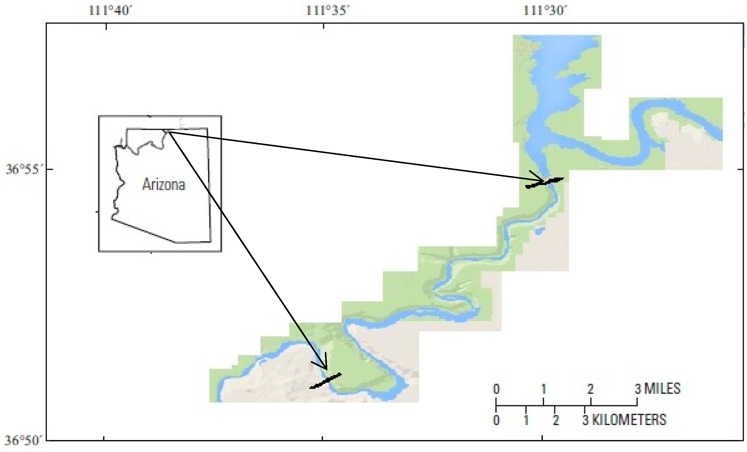
2. Study Areas and Mathematical

In this part, we developed a novel two-dimensional habitat model system. The model system consists of four parts: (1) the dynamic 2D depth-averaged hydraulics model; (2) the heat transfer model; (3) the physical habitat model based on the aforementioned steps; (4) the sensitivity analysis based on the WUA and OSI. The flow chart of the model system is shown in Figure 1, and in Figure 1 SI is short for suitability index.

2.1. Study Areas and Mathematical Description of CFD Simulations

The Colorado River stretch from Glen Canyon Dam to Lees Ferry has been used for the model application (Figure 2). The river discharge and the river bed substrates during study time are shown in Figure 3. The sediment grading curve and flow discharge are obtained based on the survey data. The river bathymetry is based on the cross-section and interpreted in the whole river stretch (Figure 4). The theodolite was used to survey the river cross-section and more than 100 sampling points were applied for the substrates. The detailed survey data description on these study areas can be found in Voichick [21], Vernieu [22], Makinster [23,24] and Yao [25,26]. In the present model system, the 2D depth-average CFD model equations used for hydraulic simulation in this study are the continuity equation, the standard k-ε turbulent viscosity model for the Navier–Stokes equation and heat transfer equations. For the depth calculation in the river, we assume that the velocity in the vertical direction is almost negligible. The equations present the variations in the mean quantities and are valid in the computational domain (ΩF). The conservation equations for both mass and momentum are presented as follows:
Continuity equation
h t + ( U h ) x + ( V h ) y = 0
Moment equation
U t + U U x + V U y = ρ g ( Z Z 0 ) x + χ U ( 2 U x 2 + 2 U y 2 ) A r T
V t + U V x + V V y = ρ g ( Z Z 0 ) y + χ U ( 2 U x 2 + 2 U y 2 ) A r T
Heat transfer equation
T t + U T x + V T y = χ U ( 2 T x 2 + 2 T y 2 )
For turbulent kinetic energy K
K t + U K x + V K y = x ( χ K K x ) + y ( χ K K y ) E G b + G k
For the dissipation rate E
E t + U E x + V E y = x ( χ E E x ) + y ( χ E E y ) C 2 E 2 K C 1 C 3 G b E K + C 1 E K G k
The kε turbulence model is based on turbulence kinetic energy (K) and the dissipation rate (E). The kε turbulence model for k is derived from the exact equation, while the kε turbulence model for ε was obtained based on physical reasoning [27,28,29]. In the kinetic energy and its dissipation rate equations, quantities Gk and Gb are the turbulent kinetic energy production due to shear and buoyancy. The Gk and Gb can be written as follows,
G k = C μ K 2 E ( U i X j + U j X i ) U i X j ,   G b = G r Re 2 C μ K 2 / E σ T T X i e g
The effective diffusion coefficients appearing in the momentum, energy and turbulence equations are described as follows,
χU = 1/Re + νtur, χT = 1/PrRe + νtur/σT, χS = 1/ScRe + νtur/σS
χK = 1/Re + νtur/σK, χE = 1.0/Re + νtur/σE
The turbulent eddy viscosity, defined as νtur = CμK2/E, was applied to measure the turbulence strength. The kε model constants Cμ, C1, C2, C3, σK, σE, σT and σS respectively and the values were shown as following,
Cμ = 0.09, C1 = 1.44, C2 = 1.92, C3 = 1.00, σK = 1.00, σE = 1.30, σT = 0.90, σS = 0.70
Turbulent Prandtl number σT and turbulent Schmidt number σS actually were expressed as function forms of the ratio of eddy to diffusivities and distance to the boundary condition. As a matter of flow properties, standard values of turbulent Schmidt and Prandtl numbers could be adopted for use in the above equations [30].
Figure 4 details the numerical modeling of flow in the river, with appropriate boundary and initial conditions. The inflowing velocity profile and temperature distribution are set. The geometry of the river (water depth) and low turbulence intensity (K = 0.3%) are also set as the initial values. The study river stretch and the bathymetry data are shown in Figure 4.
In order to solve the aforementioned model numerically, the inlet, outflow boundaries and the adiabatic wall boundary conditions were applied. The inlet condition was set by the inflow velocities (Uin), water temperature (Tin) and water depth (Hin) of the inlet boundary layer. The turbulent kinetic energy and its dissipation rate were calculated based on the following equations,
Kin(Y) = 1.50 × (10% × Uin(Y))2, Ein(Y) = Cμ0.75Kin(Y)1.5/L(Y),
where L(Y) = 151 × (Y/10)α, which represents the length scale of the velocity components along the flow direction.
In the outflow boundary, zero gradient is applied for velocities, temperature, turbulent kinetics and its dissipation rate, it can be written as mathematically.
U n = V n = K n = E n = T n = 0

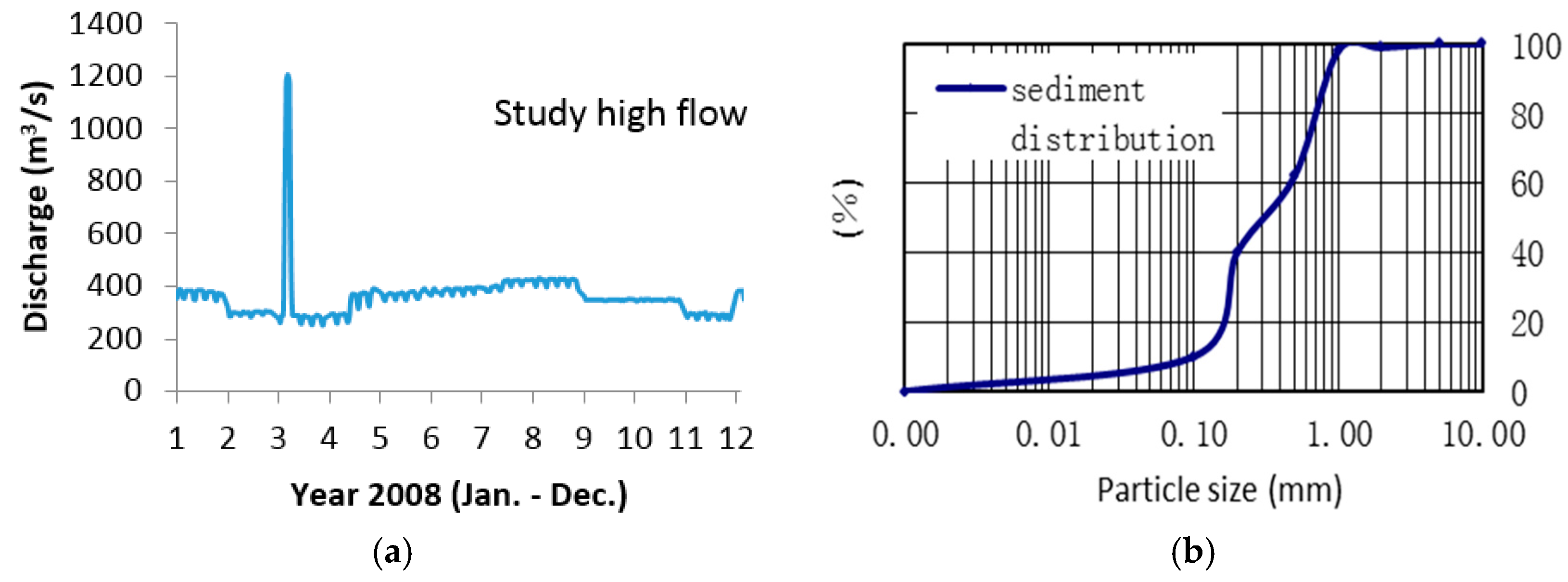
2.2. Sediment Transport

Formula for the sediment transport and river bed deformation is developed. For bed load sediment, an overall mass balance equation has been employed to ascertain the bed elevation change Zb [31]:
( 1 p ) Z b t + Q b s x + Q b n y = 0
Many semi-empirical formulae are available to calculate the bed load transport rate such as Meyer-Peter–Müller, Einstein–Brown, England–Hansen, Van Rijn equations [32,33,34,35]. Taking into account the stability of the formula and the mean diameter of graded sediment of the Meyer-Peter–Müller equation (0.4 to 29 mm), the Meyer-Peter–Müller equation has been applied:
Q e = 8 [ ( C C 90 ) 3 / 2 θ θ c r ] 3 / 2 ( ρ s ρ g d 50 3 ) 1 / 2 ; θ c r = 0.047 ;
θ = τ b ( ρ s ρ ) g d 50

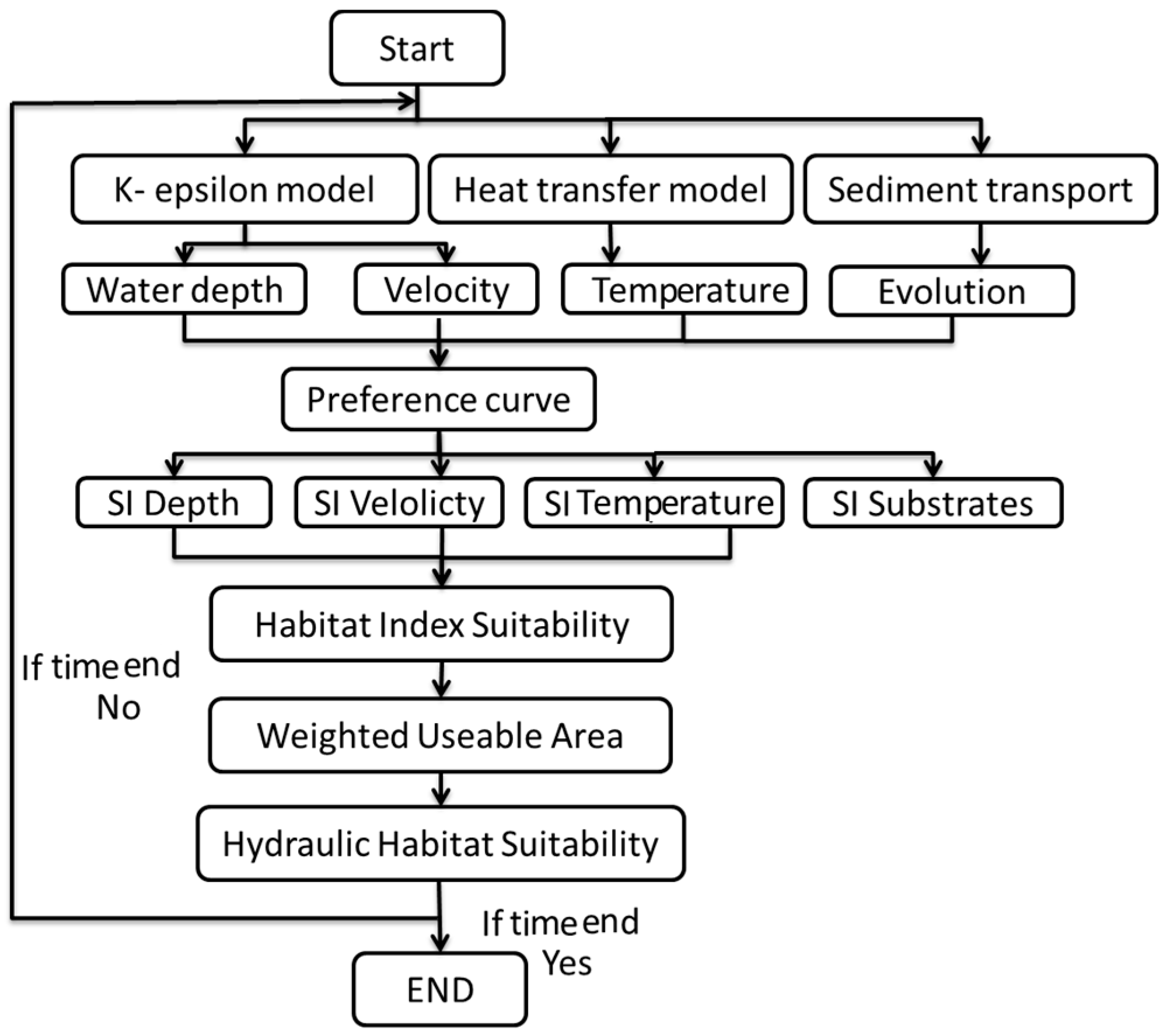
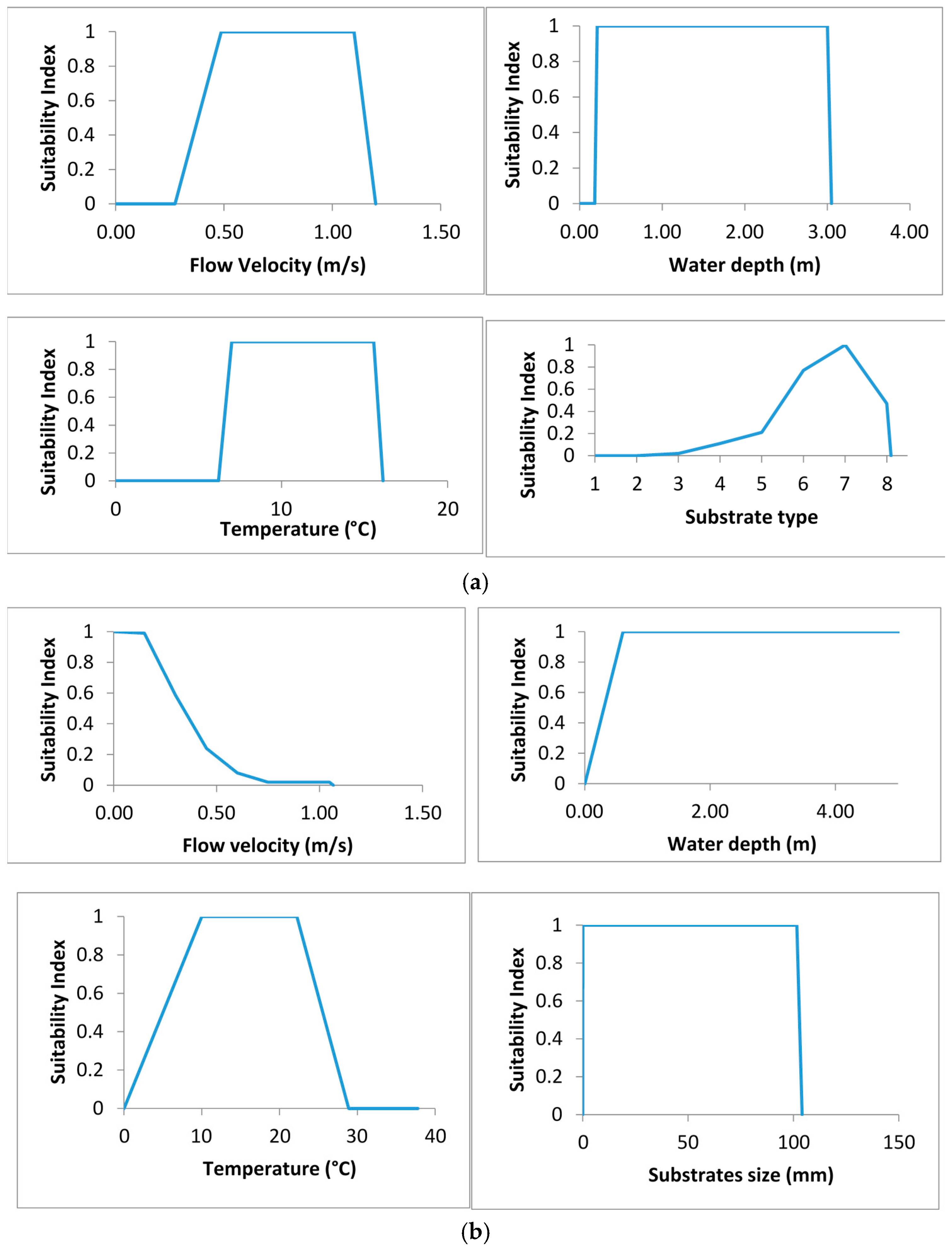
2.3. Habitat Construction

The habitat model is constructed based on the hydraulic variables from the CFD simulation and fish preference curves. Fish preference curves are, in turn, founded on literature, laboratory studies and frequency of the field observation (which has certain values within a variable range of values for fish habitat). The preference curves applied in this study are mainly taken from a specific fish study on the Colorado River and only four indices which significantly affected fish habitat were chosen [36,37,38]. These fish preference curves are specific for spawning and juvenile rainbow trout. The habitat suitability index value ranges from 1 to 0, with 1 for the highest value and 0 for the lowest value. The preference curves for study species are show in Figure 5. The habitat model is related to physical and ecological parameters for evaluating the natural and unpolluted rivers.
The physical habitat model was proposed by attributing equal weighting to variables of flow velocity, depth, water temperature, and the substrates suitability index. The habitat model is used to assess the habitat changes caused by high flow effects which are caused by the Glen Canyon Dam. The Habitat Suitability Index (HSI) equation is as follows and in order to further describe the HSI, it is divided into three classes which are high, middle and low HSI (Table 1).
HSI =   ( S I v × S I d × S I t × S I s ) 1 / 4

2.4. WUA and OSI Construction Procedure

Founded on the habitat concepts of PHABSIM and River2D [17,18,19,39], the WUA and the OSI for the fish species under a given hydraulic condition were also computed [8,40,41]. The WUA is defined as follows:
W U A =   i = 1 M A i H S I i
So as to make a comparison between different rivers, the OSI is also set up. The OSI index can be defined as the ratio of the weighted usable area to the total study area. For the river stretch, the OSI value is ranged from 1 to 0.
O S I =   i = 1 M A i H S I i i = 1 M A i

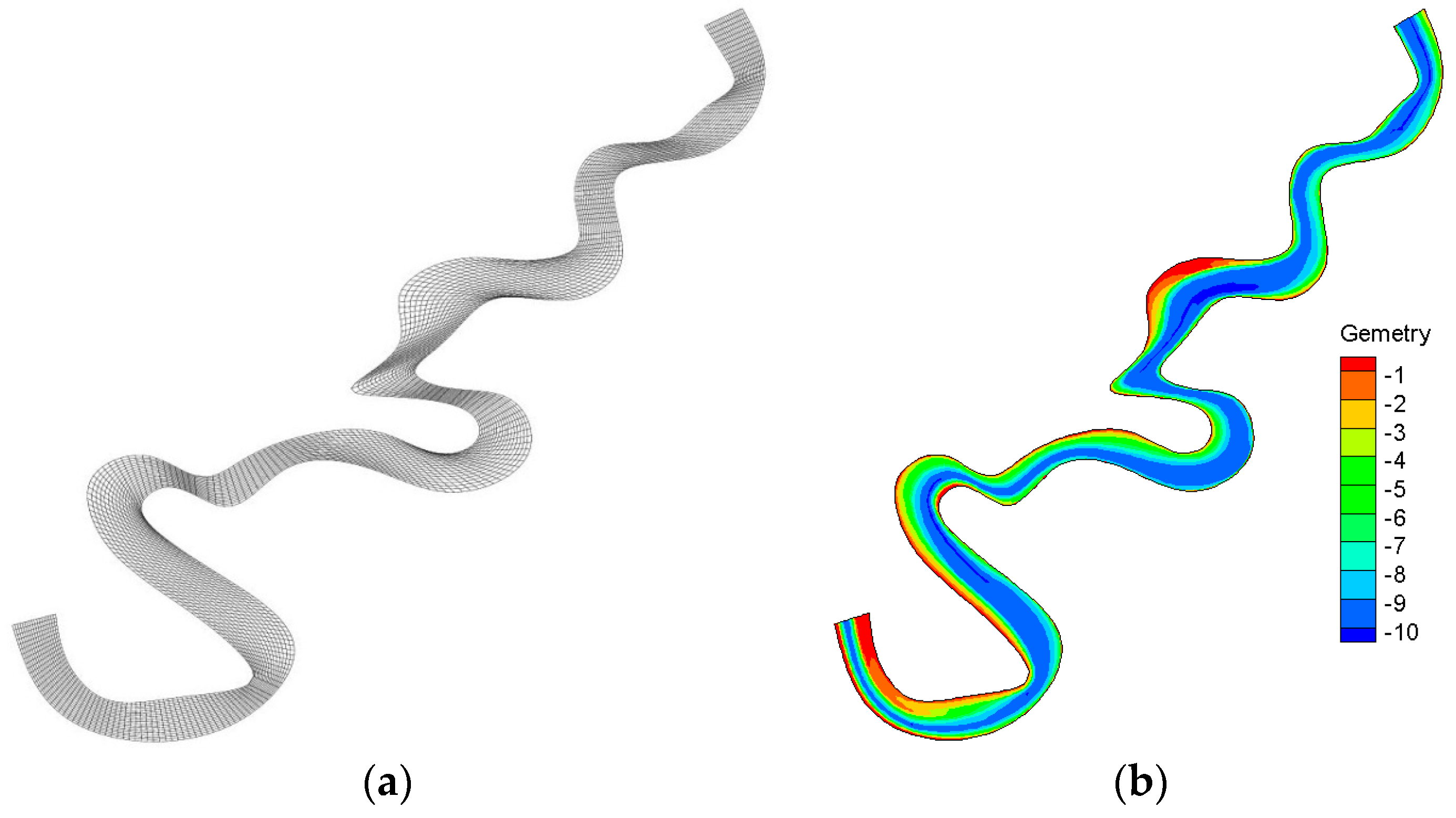
3. Numerical Model Setup and Implementation

The whole model was set up and the Finite Volume Method (FVM) was applied to solve the staggered grid system on partial differential equations. The third-order deferred correction QUICK scheme, SIMPLE iteration, tri-diagonal matrix algorithm (TDMA) and the successive over relaxation (SOR) were also applied in the CFD model [42,43].
After the turbulence and energy model is resolved by the CFD model, the parameters including flow velocity, depth and temperature distribution, and substrates are obtained. The sediment transport equations are also solved by the FVM. By coupling the HSI function and the fish preference curves together, on the grounds of computed results from the CFD module, the HSI for the fish species under study is obtained. Similarly, the WUA and OSI are also obtained based on Equations (15) and (16) on each mesh volume.
The convergence criterion is based on the maximum permissible errors in global mass and energy imbalances, which are defined as 10−9 in this model system [42]. Significance tests were conducted for the accuracy of the model system and also the dependency of solutions for grid size. More detail can be found in Yao et al. [26,44,45].

4. Results and Discussion

The site of spawning and juvenile rainbow trout living in Colorado River—stretching from downstream of the Glen Canyon Dam to Lees Ferry—was analyzed to verify the high flow effects on flow velocity, water depth, temperature and substrates on the tail water of the dam and the habitat suitability quality. The river stretch is shown in Figure 4. A mesh of 300 × 20 was used in the model system with geographic data being interpolated from a surveyed cross-section (2,550,000 m2).

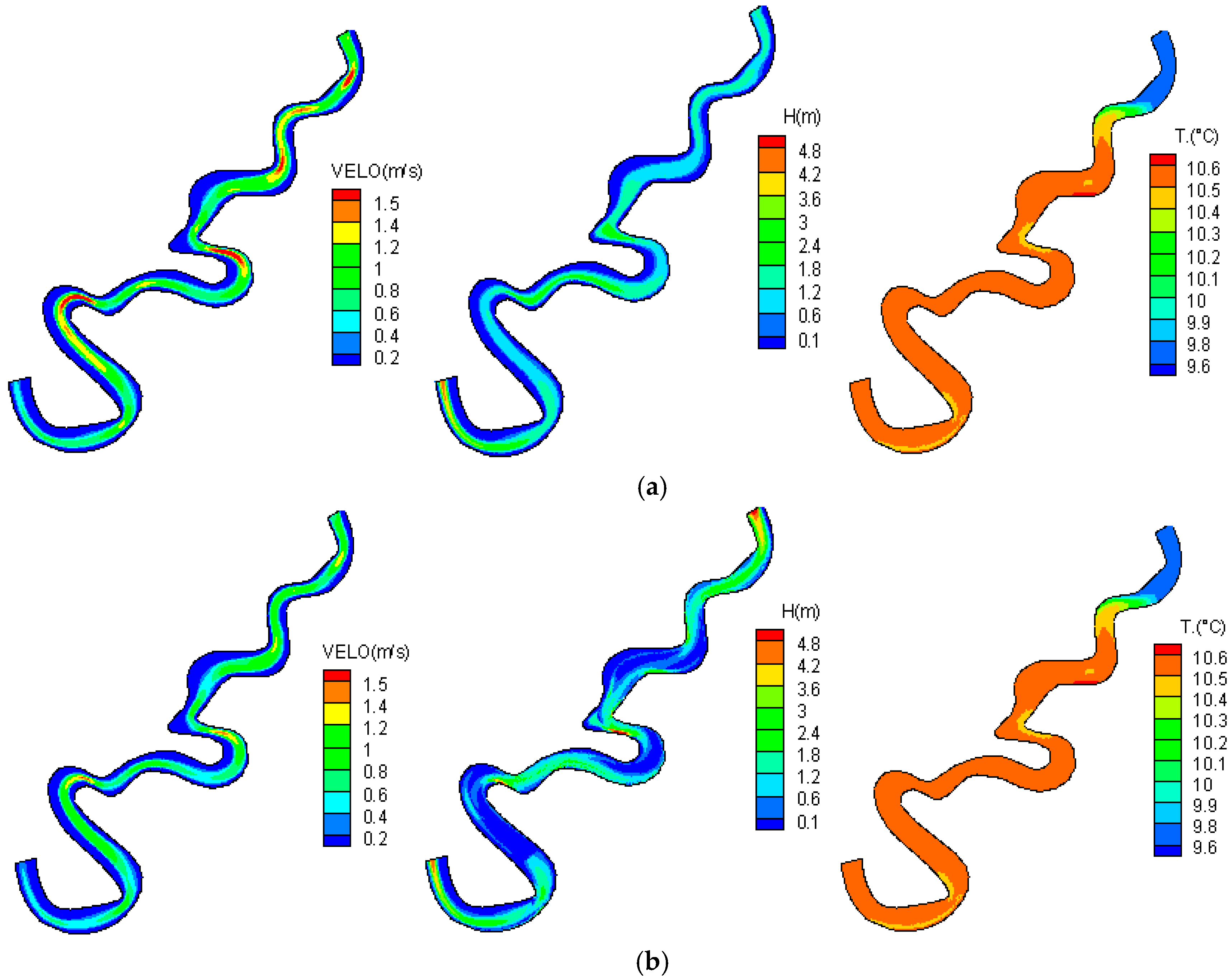
4.1. High Flow Effects on Velocity and Temperature

Figure 6 show simulated velocity, water depth and temperature before and after the HFE. From the simulation, we can notice that the velocity is relatively slow after the HFE and the highest velocity occurs in the middle of the river; the values being 1.5 m/s and 1.3 m/s, which happened at the curved and narrowest part of the river. The velocity prior to HFE ranges from 0.4 m/s to 1.5 m/s and post HFE, it ranges from 0.3 to 1.3 m/s (Figure 6b).
The flow temperature simulation outcomes are also depicted in Figure 6. From the simulation, we can interpret that prior to the start of the HFE, the temperature distribution is mostly uniform in the river (11 °C) except for the areas near to the inlet of the computational domain which has low water temperature (9.5 °C). The reason for this is that the cold water from the Glen Canyon Dam affects these areas which are near to the inlet of the river. The distance of the cold-water temperature effects is 5 km and 10 km for before HFE and during HFE respectively. Subsequent to the HFE, the temperature distribution is in no manner different than before the HFE.

4.2. Hydrodynamic Simulation Results

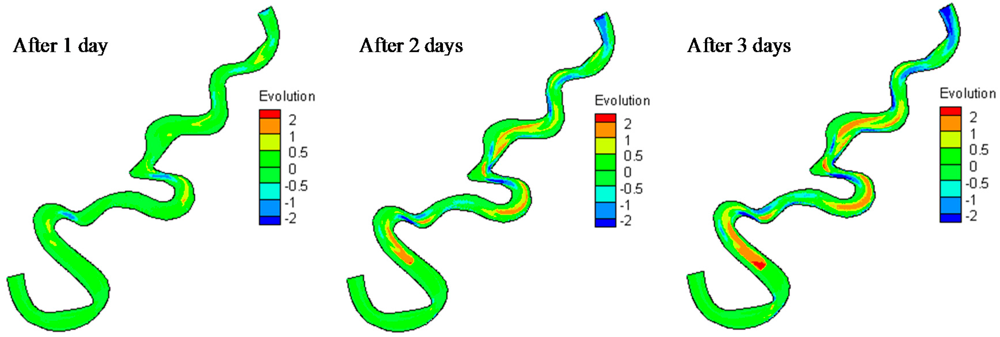
4.2.1. High Flow Effects on River Bed Elevation and Water Depth

Simulation results have been portrayed for the river bed elevation in Figure 7. It can be understood easily that after 1 day, the river bed elevation was minimal, covering almost the whole reach with positive elevation values ranging from 0.1 m to 0.25 m in the middle portions of the river. At the inlet which is also the narrowest part of the computational domain, some negative values of bed elevation were also observed with values around −1.3 m. Thereafter, positive bed elevation increased in terms of both values and area. The negative bed elevation affected areas also increased in size at the inlet and in several small patches of the computational domain with minimum values being around −1.8 m. At the end of the HFE, it can be noted that the positive bed elevation was mainly emphasized on the middle and downstream of the computation domain with a maximum value of 2 m. In contrast, negative bed elevation spread in the upstream area and near to inlet areas with a minimum value of −2.1 m.
Comparing the water depth simulation results, it appears that water depth changed on a par with river bed elevation. Before the HFE, the mean water depth in the middle of the river was 3.5 m while after the HFE, the water depth significantly increased near the inlet with a value of 4.5 m (Figure 6). The simulated velocity results are reasonable and fitted with the method proposed by Graf [46]. The simulated water depth is fitted with the previous study [47] and the simulated results of the temperature distribution are also in line with the previous study [48,49].

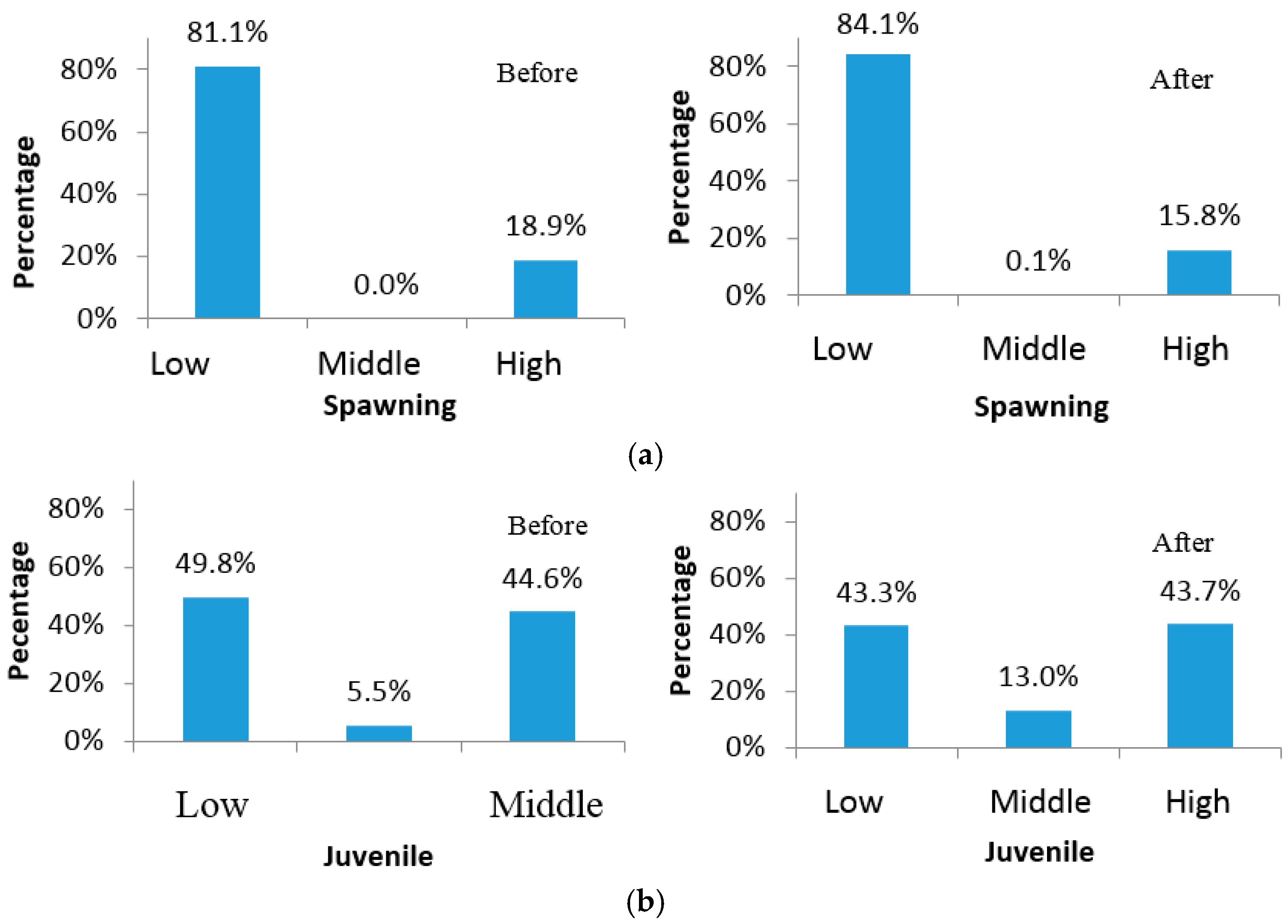
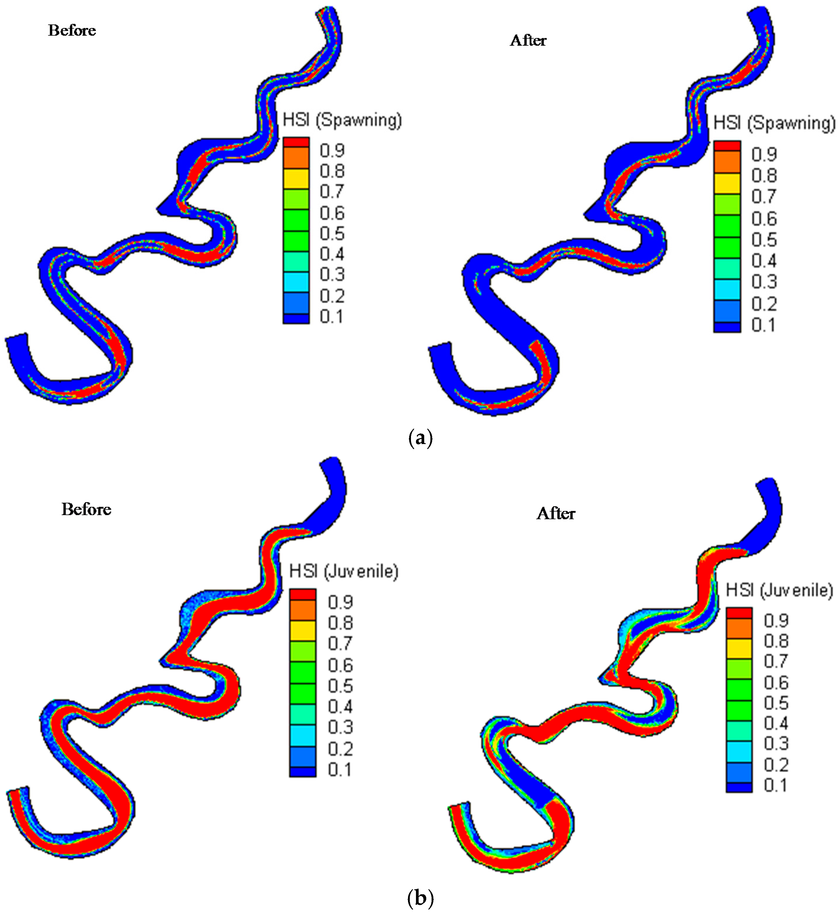
4.2.2. High Flow Effects on Spawning and Juvenile Rainbow Trout Habitat Suitability

Figure 8 shows the calculated HSI distribution for spawning and juvenile rainbow trout. The results illustrate that the HSI values for the spawning and juvenile fish are different, which is mainly due to the geomorphology changes.
More specifically, (1) before the HFE, the majority parts in the middle of the river had a high habitat suitability index for juvenile rainbow trout, except the areas near the inlet and the center of the river which had a higher value than the river sides (Figure 8a). The low HSI near the inlet is mainly because of cold water released from the bottom of the reservoir and the maximum affected distance is 10 km during the HFE. The proportion of the high, middle and low HSI for juvenile rainbow trout are 44.6%, 5.51% and 49.8% respectively (Figure 9). For the spawning stage of rainbow trout, the HSI situation is even worse than juvenile rainbow trout as only five small segments of areas have suitable habitat for spawning rainbow trout (Figure 8b). The percentage of the high, middle and low HSI for spawning rainbow trout are 18.9%, 0.02% and 81.1% respectively (Figure 9). The reason behind this is that the spawning fish require a very limited velocity range and water depth which cannot be provided in high flow situation even though the water temperature is very suitable for the spawning fish; (2) After HFE, the HSI situation for the juvenile life stage is different. To be specific, the HSI values decreased in some small fragments of areas in the middle of river while the HSI values in the river side increased in the majority of the river parts (Figure 8). The proportion of middle HSI increased to 13% while the low HSI decreased to 43.3% and the high HSI remain unchanged (Figure 9). For the spawning life stage of rainbow trout, the HFE has caused a decline in spawning habitat suitability and the percentage of high HSI declined from 18.9% to 15.8% (Figure 9).

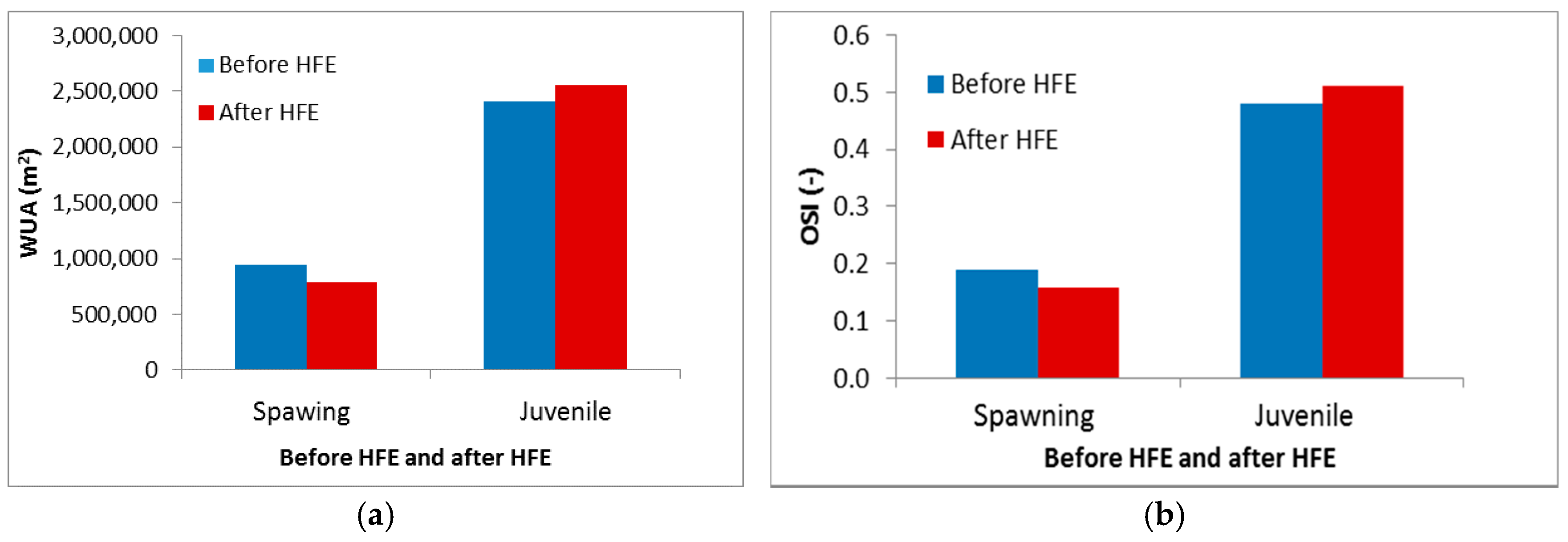
4.3. Weighted Usable Area and Overall Usable Area Analyses

The spawning and juvenile rainbow trout habitat qualities have been carried out as per the WUA and OSI based on equations 15 and 16. For juvenile rainbow trout with HFE, it is noted that the WUA increased from 2.41 × 10⁶ m2 to 2.61 × 10⁶ m2 and the OSI increased from 0.48 to 0.51 correspondingly. However, the WUA and OSI values for spawning rainbow trout are smaller than juvenile rainbow trout. With the HFE, the WUA for spawning rainbow trout were 9.46 × 10⁵ m2 and 7.91 × 10⁵ m2 and the OSI declined from 0.19 (before HFE) to 0.16 (after HFE) (Figure 10).
Table 2 displays high, middle and low WUA spawning and juvenile rainbow trout response to the HFE in the river reach from the Glen Canyon Dam to Lees Ferry in March 2008. It can be noticed that the spawning and juvenile rainbow trout effects have a huge disparity when they face the same HFE. According to Table 2, before HFE, the juvenile high and middle WUA values are more than the corresponding spawning rainbow trout WUA values with the values being 2.23 × 10⁶ m2, 2.75 × 10⁵ m2 for juvenile rainbow trout and 9.46 × 10⁵ m2, 1.03 × 10³ m2 for spawning rainbow trout respectively. After the HFE, the high WUA for spawning rainbow trout decreased to 7.90 × 10⁵ m2 while the middle and low WUA increased to 3.10 × 10³ m2 and 4.21 × 10³ m2. The high, middle and low WUA values for juvenile rainbow trout are 2.19 × 10⁶ m2, 6.51 × 10⁵ m2 and 2.16 × 10⁶ m2 respectively.
It should be noted that there are some differences between the habitat model proposed here and the other habitat models. In the habitat model proposed in this paper, the sediment transport module is included in the model and the heat transfer equation is incorporated. Both heat transfer and sediment transport modules make the habitat model much more closed to physical reality. The temperature can be moderated by hypothetic exchange flow and the flux increased by the HFE for the habitat model predictions. Notably, the indexes including the SI, HSI, WUA, and OSI are simulated simultaneously in this paper, which could provide useful information for optimizing their choices.
The features and the application of the fish habitat model indicated that the HFE was beneficial for the juvenile rainbow trout habitat, but declined the spawning rainbow trout habitat quality. In addition, during the HFE, the poor habitat quality reached 10 km. This information could help the river manager to pay special attention to these sensitive areas and also pay attention to the fish tolerance to low temperature. The habitat model used here could be used to determine whether the rainbow trout habitat construction has been affected by the HFE and what proportion of the habitat structure has been affected. This approach could also help to determine the habitat assessment standard on both natural rivers and rivers with dams. It provides guidelines for ecological monitoring status and provides inputs for the eco-hydraulic population model [50]. It should be noted that the habitat model could easily adapt to other study rivers including both HFE and non-HFE rivers. Based on the habitat model simulation, the long-term habitat quality can also be predicted.

5. Conclusions

The two-dimensional habitat models, linking the suitability curves of rainbow trout, permitted a better understanding of parameters influencing and enhancing both ecological and habitat creation. The ecological experiences integrated with the hydraulic parameters were used for calculation and calibration of the eco-hydraulics modeling. The numerical model showed encouraging outputs regarding the flow velocity, water depth and water temperature distribution. This eco-hydraulics habitat model system can be used for other fish species as well as other river stretches and/or river stretches separated by dams.
To summarize, the HFE is beneficial for the juvenile rainbow trout, but declines the habitat quality for spawning rainbow trout. It is to be noted that one potential strategy for the up-gradation of this model involves rescaling Colorado River hydrology and trying to manage key physical processes and the resulting habitat characteristics.

Acknowledgments

The work was financially support by CSC funding support (No. 201163003), China water key project plan (2016YFC0502004-4), and CAS project (Y6V60222YZ). We also thank the editor Evelyn Ning and two anonymous reviewers. They comments and suggestions help to improve the paper quality significantly.

Author Contributions

This paper has proposed by Weiwei Yao and Yuansheng Chen. This manuscripts was wrote by Weiwei Yao and Yu Zhong. The authors named Huaxian Liu, Wenyi Zhang, Haiyan Fan and Linkai Li gave constructive suggestions. Sudeep Bamal helps to improve the English expression.

Conflicts of Interest

The authors declare no conflict of interest.

Abbreviations

AiThe area of the mesh i
C e q Suspended load mass concentration at reference lever under equilibrium conditions
CFDComputational Fluid Dynamics
C r e f Suspended load concentration at reference lever
χ t Turbulence diffusivity scalar
θ Non-dimensional skin friction number/shields number
θ c r Critical shields value
v t The eddy viscosity
CChezy friction coefficient
d50Particle size parameter in 50 percent
fcorThe Coriolis parameter
gGravitational acceleration
GrGrashof number
hFluid column height
HFEHigh Flow Effect
HSIHabitat suitability index
MThe total number of grid mesh
OSIOverall suitability index
P’The non-cohesive bed porosity
Qbs, QbnBed-load flux
ReReynolds number
SIv, SId, SIs, SItSuitability index for velocity, water depth, substrates and temperature
tTime
TTemperature
U, VDepth average velocity components in x and y directions respectively
WUAWeighted usable areas
Z-Z0Water depth
ηWater surface elevation
τbBed shear stresses
τxx τxy τyx, τyyDepth-average Reynolds (turbulent) stresses
ρsSediment density
ρwWater density

References

  1. Almeida, G.; Rodríguez, J. Integrating Sediment Dynamics into Physical Habitat Models. In Proceedings of the 18th World Imacs/ModSim Congress, Cairns, Australia, 13–17 July 2009; pp. 2258–2264.
  2. McDonald, R.; Nelson, J.; Paragamian, V.; Barton, G. Modeling the effect of flow and sediment transport on white sturgeon spawning habitat in the Kootenai River, Idaho. J. Hydraul. Eng. 2010, 136, 1077–1092. [Google Scholar] [CrossRef]
  3. Wang, Z.; Lee, J.H.; Xu, M. Eco-hydraulics and eco-sedimentation studies in china. J. Hydraul. Res. 2013, 51, 19–32. [Google Scholar] [CrossRef]
  4. Bunn, S.E.; Arthington, A.H. Basic principles and ecological consequences of altered flow regimes for aquatic biodiversity. Environ. Manag. 2002, 30, 492–507. [Google Scholar] [CrossRef]
  5. Ward, J.; Tockner, K.; Schiemer, F. Biodiversity of floodplain river ecosystems: Ecotones and connectivity. Regul. Rivers Res. Manag. 1999, 15, 125–139. [Google Scholar] [CrossRef]
  6. Ward, J.V.; Stanford, J. Ecological connectivity in alluvial river ecosystems and its disruption by flow regulation. Regul. Rivers Res. Manag. 1995, 11, 105–119. [Google Scholar] [CrossRef]
  7. Wang, Y.; Xia, Z. Assessing spawning ground hydraulic suitability for chinese sturgeon (acipenser sinensis) from horizontal mean vorticity in Yangtze River. Ecol. Model. 2009, 220, 1443–1448. [Google Scholar] [CrossRef]
  8. Yi, Y.; Wang, Z.; Yang, Z. Two-dimensional habitat modeling of Chinese sturgeon spawning sites. Ecol. Model. 2010, 221, 864–875. [Google Scholar] [CrossRef]
  9. Milhous, R.T.; Wegner, D.L.; Waddle, T. User’s Guide to the Physical Habitat Simulation System (Phabism); US Fish and Wildlife Service: Washington, DC, USA, 1984.
  10. Parasiewicz, P. Mesohabsim: A concept for application of instream flow models in river restoration planning. Fisheries 2001, 26, 6–13. [Google Scholar] [CrossRef]
  11. Parasiewicz, P. Upscaling: Integrating habitat model into river management. Can. Water Resour. J. 2003, 28, 283–299. [Google Scholar] [CrossRef]
  12. Parasiewicz, P. The mesohabsim model revisited. River Res. Appl. 2007, 23, 893–903. [Google Scholar] [CrossRef]
  13. Noack, M. Modelling Approach for Interstitial Sediment Dynamics and Reproduction of Gravel-spawning Fish. Ph.D. Thesis, Universität Stuttgart, Stuttgart, Germany, 2012. [Google Scholar]
  14. Lessard, J.L.; Hayes, D.B. Effects of elevated water temperature on fish and macroinvertebrate communities below small dams. River Res. Appl. 2003, 19, 721–732. [Google Scholar] [CrossRef]
  15. Armstrong, J.; Kemp, P.; Kennedy, G.; Ladle, M.; Milner, N. Habitat requirements of atlantic salmon and brown trout in rivers and streams. Fisheries Res. 2003, 62, 143–170. [Google Scholar] [CrossRef]
  16. Bovee, K.D. A Guide to Stream Habitat Analysis Using the Instream Flow Incremental Methodology. Ifip No. 12; US Fish and Wildlife Service: Fort Collins, CO, USA, 1982.
  17. Bovee, K.D. Development and Evaluation of Habitat Suitability Criteria for Use in the Instream Flow Incremental Methodology; USDI Fish and Wildlife Service: Washington, DC, USA, 1986.
  18. Gard, M. Comparison of spawning habitat predictions of phabsim and river2d models. Int. J. River Basin Manag. 2009, 7, 55–71. [Google Scholar] [CrossRef]
  19. Gard, M. Response to Williams (2010) on Gard (2009): Comparison of spawning habitat predictions of phabsim and river2d models. Int. J. River Basin Manag. 2010, 8, 121–125. [Google Scholar] [CrossRef]
  20. Steffler, P.; Blackburn, J. River 2D Two-Dimensional Depth Averaged Model of River Hydrodynamics and Fish Habitat Introduction to Depth Averaged Modeling and User’s Manual; University of Albert: Edmonton, AB, Canada, 2002. [Google Scholar]
  21. Voichick, N.; Wright, S.A. Water-Temperature Data for the Colorado River and Tributaries between Glen Canyon Dam and Spencer Canyon, Northern Arizona, 1988–2005; U.S. Geological Survey Data Series 251; U.S. Geological Survey: Reston, VA, USA, 2007.
  22. Vernieu, W.S. Effects of the 2008 High-flow Experiment on Water Quality in Lake Powell and Glen Canyon Dam Releases, Utah-Arizona; 2331-1258; US Geological Survey: Reston, VA, USA, 2010.
  23. Makinster, A.S.; Persons, W.R.; Avery, L.A. Status and Trends of the Rainbow Trout Population in the Lees Ferry Reach of the Colorado River Downstream from Glen Canyon Dam, Arizona, 1991–2009; 2328-0328; US Geological Survey: Reston, VA, USA, 2011.
  24. Makinster, A.S.; Persons, W.R.; Avery, L.A.; Bunch, A.J. Colorado River Fish Monitoring in Grand Canyon, Arizona; 2000 to 2009 Summary; 2331-1258; US Geological Survey: Reston, VA, USA, 2010.
  25. Yao, W.; Rutschmann, P. Three high flow experiment releases from glen canyon dam on rainbow trout and flannelmouth sucker habitat in colorado river. Ecol. Eng. 2015, 75, 278–290. [Google Scholar] [CrossRef]
  26. Yao, W.; Rutschmann, P.; Bamal, S. Modeling of river velocity, temperature, bed deformation and its effects on rainbow trout (Oncorhynchus mykiss) habitat in lees ferry, colorado river. Int. J. Environ. Res. 2014, 8, 887–896. [Google Scholar]
  27. Huang, P.; Bardina, J.; Coakley, T. Turbulence modeling validation, testing, and development. NASA Tech. Memo. 1997, 110446. [Google Scholar]
  28. Launder, B.E.; Spalding, D.B. Lectures in Mathematical Models of Turbulence; Academic Press: London, UK, 1972. [Google Scholar]
  29. Launder, B.E.; Spalding, D.B. The numerical computation of turbulent flows. Comput. Methods Appl. Mech. Eng. 1974, 3, 269–289. [Google Scholar] [CrossRef]
  30. Tominaga, Y.; Stathopoulos, T. Turbulent Schmidt numbers for CFD analysis with various types of flowfield. Atmo. Environ. 2007, 41, 8091–8099. [Google Scholar] [CrossRef]
  31. Coleman, S.; Nikora, V. Exner equation: A continuum approximation of a discrete granular system. Water Resour. Res. 2009, 45. [Google Scholar] [CrossRef]
  32. Ackers, P.; White, W.R. Sediment transport: New approach and analysis. J. Hydraul. Div. 1973, 99, 2041–2060. [Google Scholar]
  33. Meyer-Peter, E.; Müller, R. Formulas for bed-load transport. In Proceedings of the 2nd Meeting of the International Association for Hydraulic Structures Research, Stockholm, Sweden, 7–9 June 1948; pp. 39–64.
  34. Van Rijn, L.C. Principles of Sediment Transport in Rivers, Estuaries and Coastal Seas; Aqua publications: Amsterdam, The Netherlands, 1993; Volume 1006. [Google Scholar]
  35. Wu, W.; Rodi, W.; Wenka, T. 3d numerical modeling of flow and sediment transport in open channels. J. Hydraul. Engin. 2000, 126, 4–15. [Google Scholar] [CrossRef]
  36. Jowett, I.G.; Davey, A.J. A comparison of composite habitat suitability indices and generalized additive models of invertebrate abundance and fish presence–habitat availability. Trans. Am. Fish. Soc. 2007, 136, 428–444. [Google Scholar] [CrossRef]
  37. Lambert, T.R.; Hanson, D.F. Development of habitat suitability criteria for trout in small streams. River Res. Appl. 1989, 3, 291–303. [Google Scholar] [CrossRef]
  38. Matthews, K.; Berg, N. Rainbow trout responses to water temperature and dissolved oxygen stress in two Southern California stream pools. J. Fish Biol. 1997, 50, 50–67. [Google Scholar] [CrossRef]
  39. Milhous, R.T.; Updike, M.A.; Schneider, D.M. Physical Habitat Simulation System Reference Manual: Version II; US Fish and Wildlife Service: Washington, DC, USA, 1989.
  40. Moir, H.; Gibbins, C.N.; Soulsby, C.; Youngson, A. Phabsim modelling of Atlantic salmon spawning habitat in an upland stream: Testing the influence of habitat suitability indices on model output. River Res. Appl. 2005, 21, 1021–1034. [Google Scholar] [CrossRef]
  41. Mouton, A.M.; Schneider, M.; Depestele, J.; Goethals, P.L.; De Pauw, N. Fish habitat modelling as a tool for river management. Ecol. Eng. 2007, 29, 305–315. [Google Scholar] [CrossRef]
  42. Ferziger, J.H.; Peric, M.; Leonard, A. Computational Methods for Fluid Dynamics (Vol. 3); Springer: Berlin, Germany, 1996. [Google Scholar]
  43. Patankar, S. Numerical Heat Transfer and Fluid Flow; CRC press: New York, NY, USA, 1980. [Google Scholar]
  44. Yao, W.; Bamal, S.; Rutschmann, P. Simulating High-Flow Effects (HFE) on River Deformation and Rainbow Trout (Oncorhynchus mykiss) Habitat; CRC Press: New York, NY, USA, 2014; pp. 2471–2476. [Google Scholar]
  45. Yao, W.W.; Kumar, V.; Rutschmann, P. Simulating Dam Effects on River Deformation and Rainbow Trout (Oncorhynchus mykiss) Population Number; CRC press: New York, NY, USA, 2014; pp. 2477–2483. [Google Scholar]
  46. Graf, J.B. Measured and predicted velocity and longitudinal dispersion at steai) y and unsteady flow, colorado river, glen canyon dam to lake mead. JAWRA J. Am. Water Resour. Assoc. 1995, 31, 265–281. [Google Scholar] [CrossRef]
  47. Korman, J.; Kaplinski, M.; Melis, T.S. Effects of High-Flow Experiments from Glen Canyon Dam on Abundance, Growth, and Survival Rates of Early Life Stages of Rainbow Trout in the Lees Ferry Reach of the Colorado River; 2331-1258; US Geological Survey: Reston, VA, USA, 2010.
  48. Rosi-Marshall, E.J.; Kennedy, T.A.; Kincaid, D.W.; Cross, W.F.; Kelly, H.A.; Behn, K.A.; White, T.; Hall, R.O., Jr.; Baxter, C.V. Short-Term Effects of the 2008 High-Flow Experiment on Macroinvertebrates in Colorado River Below Glen Canyon Dam, Arizona; 2331-1258; US Geological Survey: Reston, VA, USA, 2010.
  49. Wright, S.A.; Anderson, C.R.; Voichick, N. A simplified water temperature model for the colorado river below glen canyon dam. River Res. Appl. 2009, 25, 675–686. [Google Scholar] [CrossRef]
  50. Yao, W. Application of the Ecohydraulic Model on Hydraulic and Water Resources Engineering. Ph.D. Thesis, Technische Universität München, München, Germany, 2016. [Google Scholar]
Figure 1. Flow chart of the model structure of this project.
Water 09 00150 g001
Figure 2. Photogrammetric base map of the study site of the Colorado River, which extends from Glen Canyon Dam to the Lees Ferry.
Water 09 00150 g002
Figure 3. Daily mean discharge released from the Glen Canyon Dam during high flow effects in 2008 (a) and sediment distribution in the river bed during high flow effects in 2008 (b).
Water 09 00150 g003
Figure 4. Study area mesh (a) and the bathymetry data of the river stretch (b).
Water 09 00150 g004
Figure 5. Spawning (a) and juvenile (b) rainbow trout flow velocity, water depth, temperature and substrates preference curves. (Substrates types: 1 = plant detritus/organic material, 2 = mud/soft clay, 3 = silt (particle size < 0.062 mm), 4 = sand (particle size 0.062 to 2.000 mm), 5 = gravel (particle size 2.0 to 64.0 mm), 6 = cobble/rubble (particle size 64.0 to 250.0 mm), 7 = boulder (particle size 250.0 to 4000.0 mm), 8 = bedrock (solid rock)).
Water 09 00150 g005
Figure 6. Simulation output of the velocity, water depth and temperature distribution before the high flow effect (HFE) (a) and after the HFE (b). (VELO = velocity; H = water depth; T. = temperature; HFE = high flow effect).
Water 09 00150 g006
Figure 7. River bed elevations after 1, 2 and 3 days.
Water 09 00150 g007
Figure 8. Before the HFE and after the HFE habitat suitability index distribution for spawning (a) and juvenile (b) rainbow trout.
Water 09 00150 g008
Figure 9. Before the HFE and after the HFE high, middle and low habitat suitability index distribution for spawning (a) and juvenile (b) rainbow trout.
Water 09 00150 g009
Figure 10. Before the HFE and after the HFE weighted usable areas (WUA) and overall suitability index (OSI) for spawning rainbow trout (a) and juvenile rainbow trout (b).
Water 09 00150 g010
Table 1. High, middle and low classification for HSI.
HSIHigh0.7–1.0
Middle0.3–0.7
Low0–0.3
Table 2. Description of the spawning and juvenile rainbow trout weighted usable area with the habitat suitability index larger than 0.7, 0.3–0.7 and 0–0.3 (Total area is 2,550,000 m2).
Habitat CategorySpawningJuvenile
WUABeforeHigh9.46 × 1052.23 × 106
Middle1.03 × 1032.75 × 105
Low4.05 × 1062.49 × 106
AfterHigh7.90 × 1052.19 × 106
Middle3.10 × 1036.51 × 105
Low4.21 × 1062.16 × 106

