Multi-Model Grand Ensemble Hydrologic Forecasting in the Fu River Basin Using Bayesian Model Averaging

Abstract

Statistical post-processing for multi-model grand ensemble (GE) hydrologic predictions is necessary, in order to achieve more accurate and reliable probabilistic forecasts. This paper presents a case study which applies Bayesian model averaging (BMA) to statistically post-process raw GE runoff forecasts in the Fu River basin in China, at lead times ranging from 6 to 120 h. The raw forecasts were generated by running the Xinanjiang hydrologic model with ensemble forecasts (164 forecast members), using seven different “THORPEX Interactive Grand Global Ensemble” (TIGGE) weather centres as forcing inputs. Some measures, such as data transformation and high-dimensional optimization, were included in the experiment after considering the practical water regime and data conditions. The results indicate that the BMA post-processing method is capable of improving the performance of raw GE runoff forecasts, yielding more calibrated and sharp predictive probability density functions (PDFs), over a range of lead times from 24 to 120 h. The analysis of percentile forecasts in two different flood events illustrates the great potential and prospects of BMA GE probabilistic river discharge forecasts, for taking precautions against severe flooding events.

1. Introduction

Ensemble forecasts from a single ensemble prediction system (EPS)/model only account for some of the uncertainties in initial conditions and model physics [1]. Other sources of uncertainty, arising from numerical implementations and data assimilation, can only be addressed by a grand ensemble (GE), which refers to a combination of several different EPSs/models [2]. Therefore, multi-model GE prediction systems have become a basis for probabilistic weather forecasts at many operational centres [3,4,5,6]. Recently, there has been a move to integrate this GE of weather forecasts into coupled meteorological-hydrological modelling systems, in order to provide improved early flood warnings [7]. Pappenberger et al. [8] applied seven meteorological EPSs to the European Flood Alert System (EFAS), to hindcast the October 2007 flooding event in the Danube basin. He et al. [9] extracted daily precipitation data from six different numeric weather prediction systems (NWPs), to drive the Xinanjiang hydrologic model for forecasting river discharges during three summer flood events in the Huai River catchment. Xu et al. [10] built a coupled meteorological-hydrological cascade system, driven by multi-model GE meteorological forecasts, to provide early flood warnings for the Linyi watershed. However, most of these studies are based on a simple assumption: all ensemble members are equally likely, and ensemble size is irrelevant, that is, the multi-model GE hydrologic predictions are formed by merging the individual runoff forecasts with equal weight. Such a simple arithmetic averaging method often cannot lead to good forecasting results, as it does not make full use of all the information available to the ensemble members [11].

Bayesian model averaging (BMA), proposed by Raftery et al. [12], is a statistical method for post-processing the ensemble forecasts of dynamic models. It generates probabilistic forecasts in the form of predictive probability density functions (PDFs), by combining several individual forecasts from different models. This approach is primarily developed for weather quantities that can be approximated by a normal distribution (surface temperature and sea level pressure) [12,13,14], which have then been extended by Sloughter et al. [15] and Sloughter et al. [16], in order to deal with skewed weather quantities (quantitative precipitation and wind speed). Studies of applications of the BMA method in meteorological forecasts indicate that the BMA post-processed PDFs are more accurate and reliable than the unprocessed ensemble forecasts [11,13,17,18,19]. However, relevant research within the domain of watershed hydrologic forecasts, and on a smaller time scale (several hours), is still very limited [20,21,22].

The primary aim of this study is to explore the effectiveness and efficiency of the BMA post-processing method for multi-model GE hydrologic predictions. In the present study, the BMA method was applied for post-processing the raw GE runoff predictions, which were obtained by running the Xinanjiang hydrologic model with meteorological inputs from seven different EPSs, to set up a BMA GE probabilistic runoff forecasting experiment in the Fu River basin in China. Following this, some improvement measures, such as high-dimensional optimization, were taken in order to complete and perfect the experiment. Finally, the results of the experiment were analyzed and evaluated, using three aspects: verification metrics, BMA weights, and percentile forecasts. Note that all of the analysis completed in this study was implemented using the statistical software package, R.

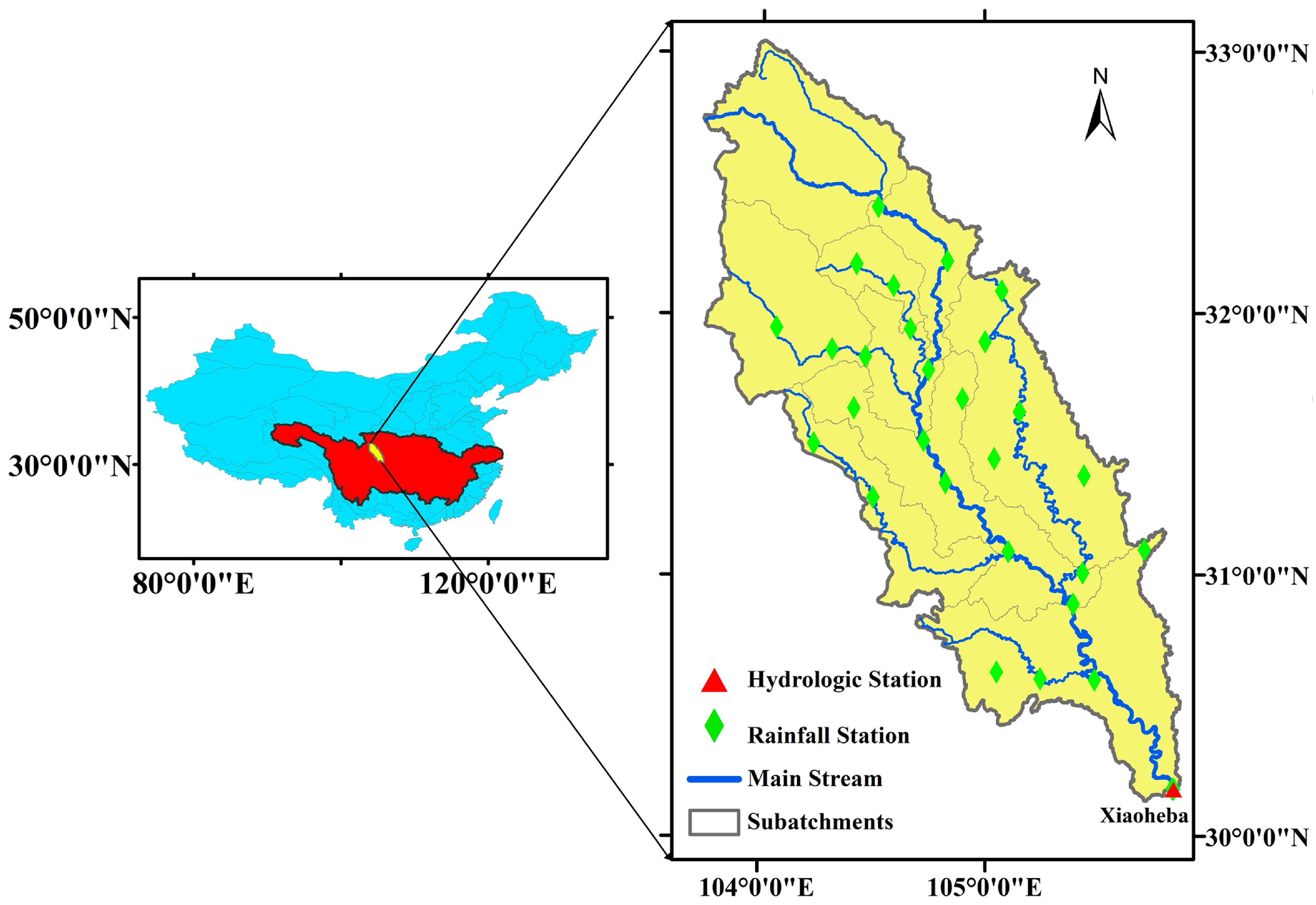
2. Study Area and Data

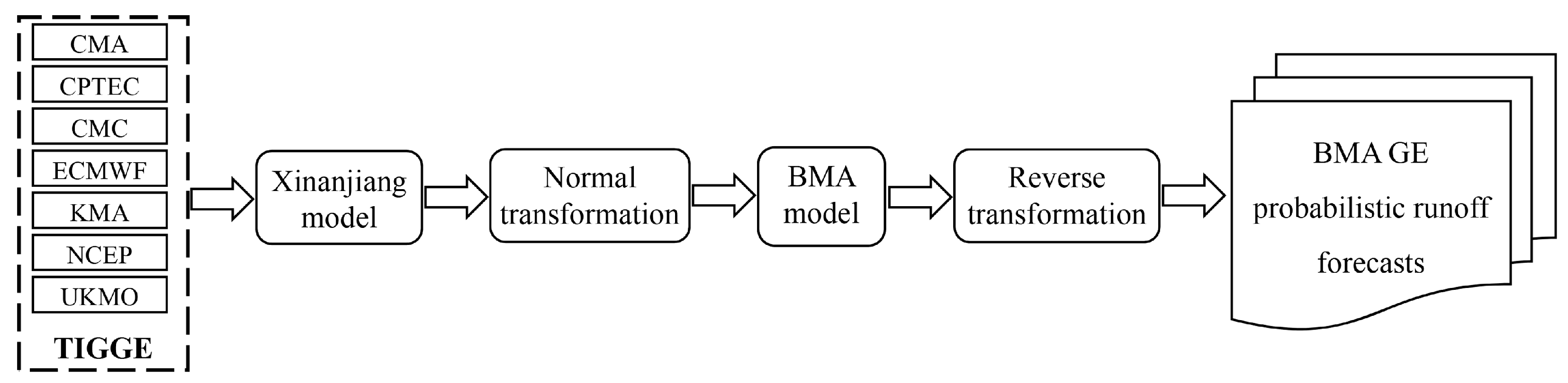
The Fu River is located in the upper reaches of the Yangtze River in China, and drains along an elongated catchment area of about 28,900 km² (Figure 1). The basin topography is varied and complicated, with a high-lying north-west, but south-eastern low. The upstream regions are mainly covered by mountains, with the highest peak being 5513 m above sea level (a.s.l). Correspondingly, the midstream and downstream areas are dominated by hills and plains, ranging from 200 to 600 m a.s.l. The precipitation is abundant, but unevenly distributed in time and space, mainly falling in the period from June to September, which accounts for more than 70% of the total annual precipitation; of which the maximum precipitation usually appears in the July. Due to the rare occurrence of snow and ice melting, the water supply of catchment runoff is mainly from rainfall. Thus, as a result, flooding disasters occur frequently in the summer months. Consequently, a dense hydrologic remote-measuring gauge network (Figure 1) has been built by the Changjiang Water Resources Commission (CWRC).

In this study, the runoff observations were provided by the CWRC. Furthermore, the runoff predictions, which serve as raw forecasts for the BMA post-processing model, were obtained by the Xinanjiang hydrologic model [23,24]. The China Meteorological Administration (CMA), Centro de Previsão de Tempo e Estudos Climáticos (CPTEC), Canadian Meteorological Centre (CMC), European Centre for Medium-Range Weather Forecasts (ECMWF), Korea Meteorological Administration (KMA), National Centers for Environmental Prediction (NCEP), and Met Office (UKMO) EPS precipitation forecasts, at lead times of 6–120 h, and extracted from the “THORPEX Interactive Grand Global Ensemble” (TIGGE) data archive [25,26], were used as the input of the Xinanjiang model; detailed descriptions of the seven TIGGE EPSs are listed in

Table 1. Meteorological ensemble forecast systems used in this study.

Centre	Country/Domain	Horizontal Resolution	Ensemble Members (Perturbed)	Forecast Length (Hours)
CMA	China	TL213	14	240
CPTEC	Brazil	T126	14	360
CMC	Canada	0.9° × 0.9°	20	384
ECMWF	Europe	TL399 (up to day 10)	50	360
KMA	Korea	N320	23	288
NCEP	United States	T126	20	384
UKMO	United Kingdom	N126	23	360

Note: For this study only the first 120 h of lead times were used.

. Corresponding to the meteorological forcing, the Xinanjiang model was run on a daily basis, initialized at 00:00 coordinated universal time (UTC), leading to a raw GE formed by 164 runoff forecast members for each time. The test period ran from 1 June to 31 August 2011.

3. Methods

The experiments used for the production of the BMA probabilistic forecasts are designed by cascading several relevant components. For this study, the main components are a TIGGE database, the Xinanjing model, data transformation (both normal transformation and reverse transformation), and the BMA model (Figure 2). The Xinanjiang model, developed by Hohai University in the 1970s, is the most widely used conceptual rainfall-runoff model in China. The main characteristic of the model is the concept of runoff formation on the repletion of storage, which implies that it is suitable for humid and semi-humid regions. The model accepts precipitation and potential evaporation data as forcing inputs, and it is usually calibrated using the Shuffled Complex Evolution method (SCE-UA) [27]. More details relating to the Xinanjiang model can be found in the work of Zhao [23] and Zhao, Liu, and Singh [24]. The following text will focus on the last two components: the BMA model and data transformation.

3.1. Bayesian Model Averaging (BMA) Model

BMA is a way of combining predictions from different sources. The generated predictive PDF can be represented as a weighted average of the conditional PDFs associated with individual ensemble forecasts $f_k(k=1,2,...,K)$:

$$p\left[y|\left(f_1,...,f_k\right)\right]={\displaystyle \sum _{k=1}^K{w}_k}{g}_k(y|f_k),$$

(1)

where $y$ is the predictive variable, $g_k\left(y|f_k\right)$ is the conditional PDF of $y$, given that $f_k$ performs best in the ensemble, and $w_k$ is the weight, which reflects the relative contribution of forecast member $k$ to the overall predictive skill demonstrated during the training period. All of the weights are non-negative and ${\displaystyle \sum _{k=1}^K{w}_k}=1$. The original BMA method is used for a situation in which the conditional PDFs of weather variables can be well-fitted by a normal distribution, centered at a linear function of the forecast, $a_k+b_k{f}_k$. In this case, the $g_k\left(y|f_k\right)$ can be expressed as a normal PDF, with a mean $a_k+b_k{f}_k$ and standard deviation ${\sigma }_k$:

$$y|f_k\sim N\left(a_k+b_k{f}_k,{\sigma }_k^2\right),$$

(2)

where $a_k$ and $b_k$ are the bias-correction terms. The BMA predictive mean can be computed by:

$$E\left[y|\left(f_1,...,f_k\right)\right]={\displaystyle \sum _{k=1}^K{w}_k}\left(a_k+b_k{f}_k\right),$$

(3)

If we denote time with subscript $t$, $f_{kt}$ denotes the forecast $f_k$ at time $t$. The BMA predictive variance can be computed by:

$$\mathrm{var}\left[y_t|(f_{1t},...,f_{kt})\right]={\displaystyle \sum _{k=1}^K{w}_k{\left[\left(a_k+b_k{f}_{kt}\right)-{\displaystyle \sum _{l=1}^K{w}_l\left(a_l+b_l{f}_{lt}\right)}\right]}^2+{\displaystyle \sum _{k=1}^K{w}_k{\sigma }_k^2}},$$

(4)

It is shown, on the right-hand side of Equation (4), that the BMA variance consists of two terms: the first one represents the between-forecast variance, and the second one represents the within-forecast variance.

The parameters and weights which need to be determined in the above equations involve: $a_k,b_k,w_k,{\sigma }_k\left(k=1,2,...,K\right)$. $a_k$ and $b_k$ are estimated by logistical regression, which is:

$$y_k=a_k+b_k{f}_k,$$

(5)

$w_k$ and ${\sigma }_k$ are estimated by using the maximum likelihood. Assuming that the forecasting errors are independent of the time domain, the log-likelihood function for the BMA model is:

$$l\left(w_1,...,w_k;{\sigma }_1^2,...,{\sigma }_k^2\right)={\displaystyle \sum _t\log \left({\displaystyle \sum _{k=1}^K{w}_k{g}_k\left(a_k+b_k{f}_{kt},{\sigma }_k^2\right)}\right)},$$

(6)

Unfortunately, there are no analytical solutions for maximizing the log-likelihood function. Instead, iterative techniques are usually resorted to, in order to deal with this problem [11]. Two of the most common methods, the Expectation-Maximization (EM) [12,28,29] and the Markov Chain Monte Carlo (MCMC) algorithms [30,31], have their own merits and demerits. In this study, the EM algorithm was selected, on account of its high computation efficiency. Note that for the BMA model, there is an implicit assumption that lead times are completely independent, that is to say, that the BMA parameters and weights for each lead time are totally irrelevant and need to be estimated separately [19,22,32].

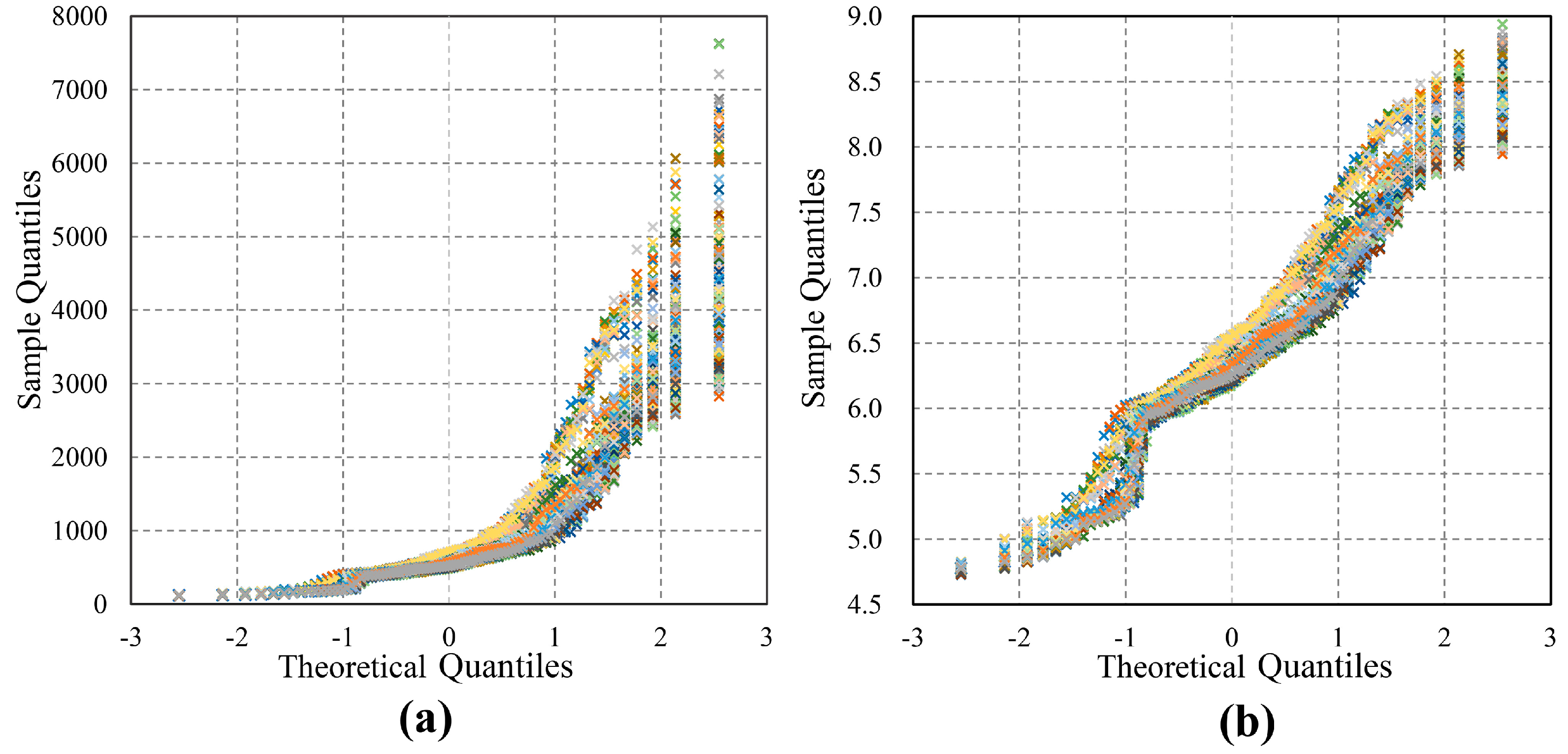
3.2. Data Transformation

Streamflow data are no doubt non-normal [20,22,33]. It has been found, upon examination, that the raw ensemble predictions used in this study followed a generalized extreme value (GEV) distribution. To satisfy the assumption of normal distribution in the BMA model, all of the data include observations and forecasts that have to be transformed in order to be approximately normal. The Box-Cox transformation [34], as a data transformation technique, has been proven to be highly effective and efficient in related studies. It is denoted by:

$$y^{\left(\lambda \right)}=\{\begin{array}{l}\frac{y^{\lambda }-1}{\lambda },\lambda \ne 0\\ \log \left(y\right),\lambda =0\end{array},$$

(7)

where $y$ is the original data, $y^{\lambda }$ is the transformed data, and $\lambda$ is the Box-Cox coefficient, which is the only parameter that needs to be determined. The BMA post-processed observations and forecasts can be reverted to the original space, through the back-transformation form of Equation (7).

3.3. Verification Metrics

The goal of probabilistic forecasts is to maximize sharpness, subject to calibration. Calibration refers to the statistical consistency between the forecasts and the associated observations, and sharpness refers to the concentration of the predictive distribution [35]. In this study, the mean absolute error (MAE), the continuous ranked probability score (CRPS), and the average width of the prediction intervals (WPI) were applied, in order to individually, and simultaneously, measure calibration and sharpness [22]. The MAE can be used to assess calibration, and is defined as:

$$MAE=\frac{1}{N}{\displaystyle \sum _{i=1}^N\left|f_i-o_i\right|},$$

(8)

where $f_i$ is the deterministic forecast value, $o_i$ is the corresponding observed value, and $N$ is the total number of observations. Note that the deterministic forecasts in this study are specified as the median forecasts (the 50th percentile forecasts), instead of the mean forecasts, in accordance with Sloughter et al. [15]. The CRPS is a measure of the difference between the predicted, and the observed, cumulative distribution [36,37], and it can take into account both calibration and sharpness. The CRPS is specified as:

$$CRPS=\frac{1}{N}{\displaystyle \sum _{i=1}^N{\displaystyle {\int }_{-\infty }^{+\infty }{\left(F_i\left(x\right)-H\left(x-o_i\right)\right)}^2}}dx$$

(9)

where $F_i\left(x\right)$ is the forecast cumulative distribution function (CDF), and $H\left(x-o_i\right)$ is the Heaviside function, that takes zero when $x<o_i$, and one otherwise. The WPI is a simple but effective measure of sharpness. Generally, it refers to the average width of a 90% prediction interval. The WPI is given by:

$$WPI=\frac{1}{N}{\displaystyle \sum _i^N\left(f_i^u-f_i^l\right)},$$

(10)

where $f_i^u$ and $f_i^l$ denote the upper and lower bound of the 90% prediction interval, respectively (namely, the 95th and 5th percentile forecasts).

It is worth noting that all three of the verification metrics conform to a law: the smaller the values, the better the forecasting results. The best possible value is zero, for a situation in which the forecast equals the observation.

4. Results and Discussion

4.1. Experiment Completion and Perfection

To complete the BMA GE probabilistic runoff forecasting experiment, the parameters of Box-Cox transformation and the BMA model have to be estimated, based on the practical hydrologic regime and data condition. In addition, the BMA model described above is a standard method that does not take into account the special circumstance (high-dimentional data space) in this study, that might bring about a serious impact on the forecasting results. So, it is necessary to take some improvement measures in order to deal with the problems, and perfect the experiment.

4.1.1. Estimation of the Box-Cox Coefficient

The runoff data cannot be successfully transformed to normal distribution and back-transformed to original space, unless a proper estimate of the Box-Cox coefficient (also the parameter) $\lambda$ is achieved. For this end, we computed and optionally plotted the profile log-likelihoods for the parameters of the Box-Cox power transformation, using the package Mass. The results showed that zero is the common optimal estimate for all ensemble members and observations. Thus, we chose the Box-Cox coefficient, $\lambda =$ 0. Figure 3 displays the normal probability plots of the original and Box-Cox transformed runoff data, at a lead time of 48 h. It is clear that the original data were successfully transformed to be approximately normal. Moreover, the Kolmogorov-Smirnov test [38] on the transformed runoff data, validated that this parameter scheme is feasible and effective.

4.1.2. Optimization of the High-Dimensional Data Space

The selected BMA parameter estimation method, the EM algorithm, is simple and fast in computation. However, this approach also falls easily into the local optimal BMA weights and variances, and becomes problematic, especially for high-dimensional data spaces (containing numerous different forecast members) [11]. For this study, with a multi-model GE consisting of 164 forecast members, it is obviously inapplicable, unless measures for reducing the number of different ensemble members are taken.

Ensemble members that lack independently distinguishable physical features (e.g., sourcing from the same prediction system/model), should be treated as exchangeable, and thus should have equal BMA parameters and weights [39]. The raw GE runoff forecasts in this study were generated by using seven different TIGGE EPSs/models, so we considered the ensemble members, derived from the same EPSs, as exchangeable. As a result, only seven sets of parameters and weights ($a_k,b_k,w_k,{\sigma }_k\left(k=1,2,...,7\right)$) remained to be determined using the BMA model. Furthermore, this strategy, to a certain extent, cut the amount of data needing to be calculated and shortened the computation time.

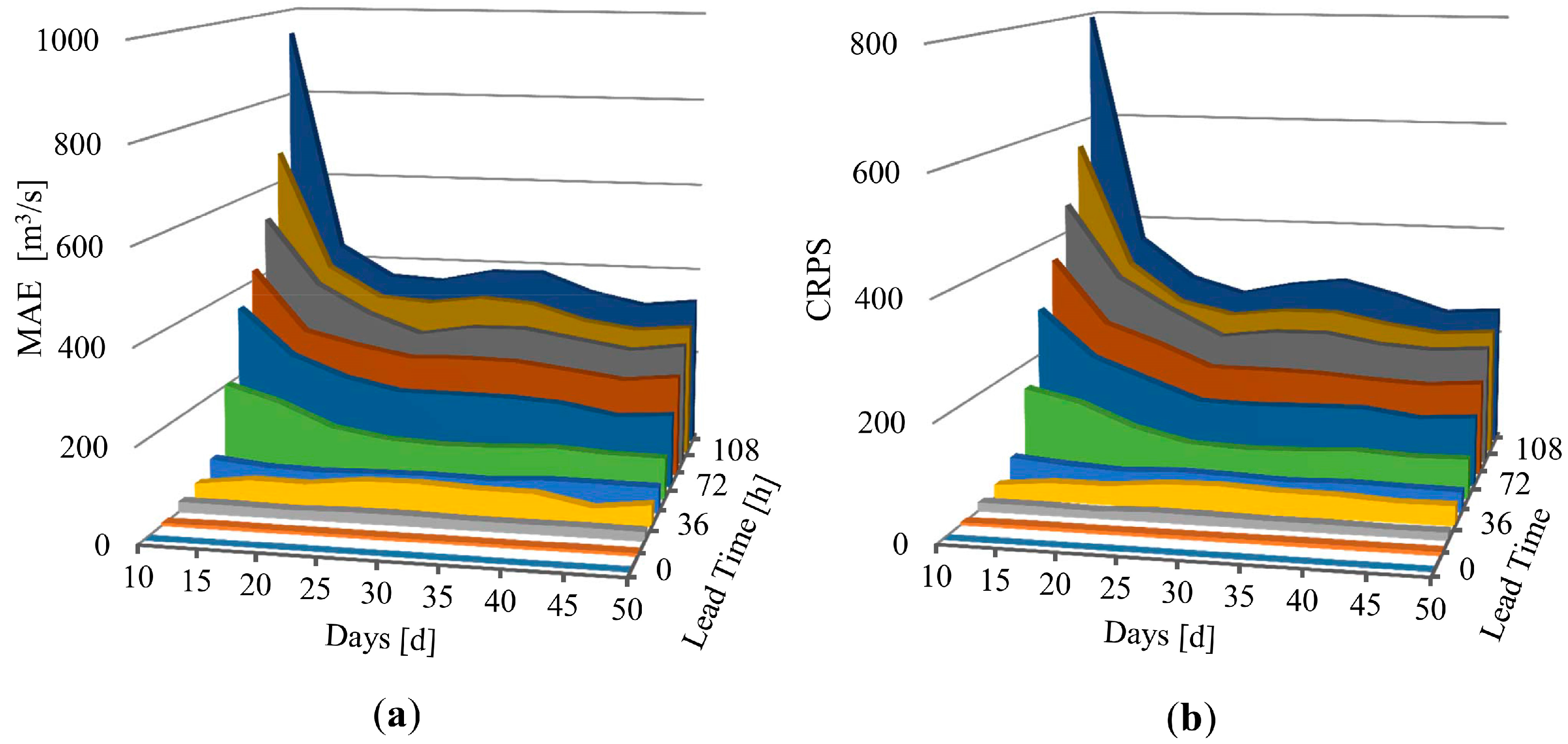
4.1.3. Estimation of the Length of Training Period

The parameter estimation for the BMA model is based on the training data, which consists of $N$ days (training period) of forecast and observation data, prior to initialization. The training period is a sliding window, and the parameters and weights are recalibrated at each new initialization time [12,15]. Among the majority of the past study cases, $N=$ 30 days was generally used as the length of the training period [15,22,32,39]. However, it is not constant and always changes for various predictive variables and study areas. To determine the length of the training period, we computed the mean MAE and CRPS of BMA GE runoff forecasts, for a list of possible training period lengths ($N=$ 10, 15, 20, 25, 30, 35, 40, 45, 50) over an entire range of lead times, up to 120 h. The period from 25 July to 31 August 2011 serves as the verification period. It is shown in Figure 4 that both MAE and CRPS have similar change features for each lead time: they both drop substantially as the number of training days increases up to 25 days, then fluctuate up and down, before declining until 45 days, and finally stabilizing. In short, BMA GE runoff forecasts reach their optimal performance while the length of the training period is greater than, or equal to, 45 days. After a synthetic consideration of the comparative results and the computation amount, we chose the length of the training period, $N=$ 45 days. Following this, the BMA parameters and weights for each lead time (6–120 h) were separately calibrated, and the building of the BMA GE probabilistic runoff forecasting experiment in the study area was then accomplished.

4.2. Forecast Performance Evaluation

In the following subsections, the performance of BMA GE probabilistic runoff forecasts at lead times of 6–120 h were verified and analyzed, using three aspects: verification metrics, weights, and percentile forecasts. The verification period lasted from 25 July to 31 August 2011, and is the same as that used in Section 4.1.3.

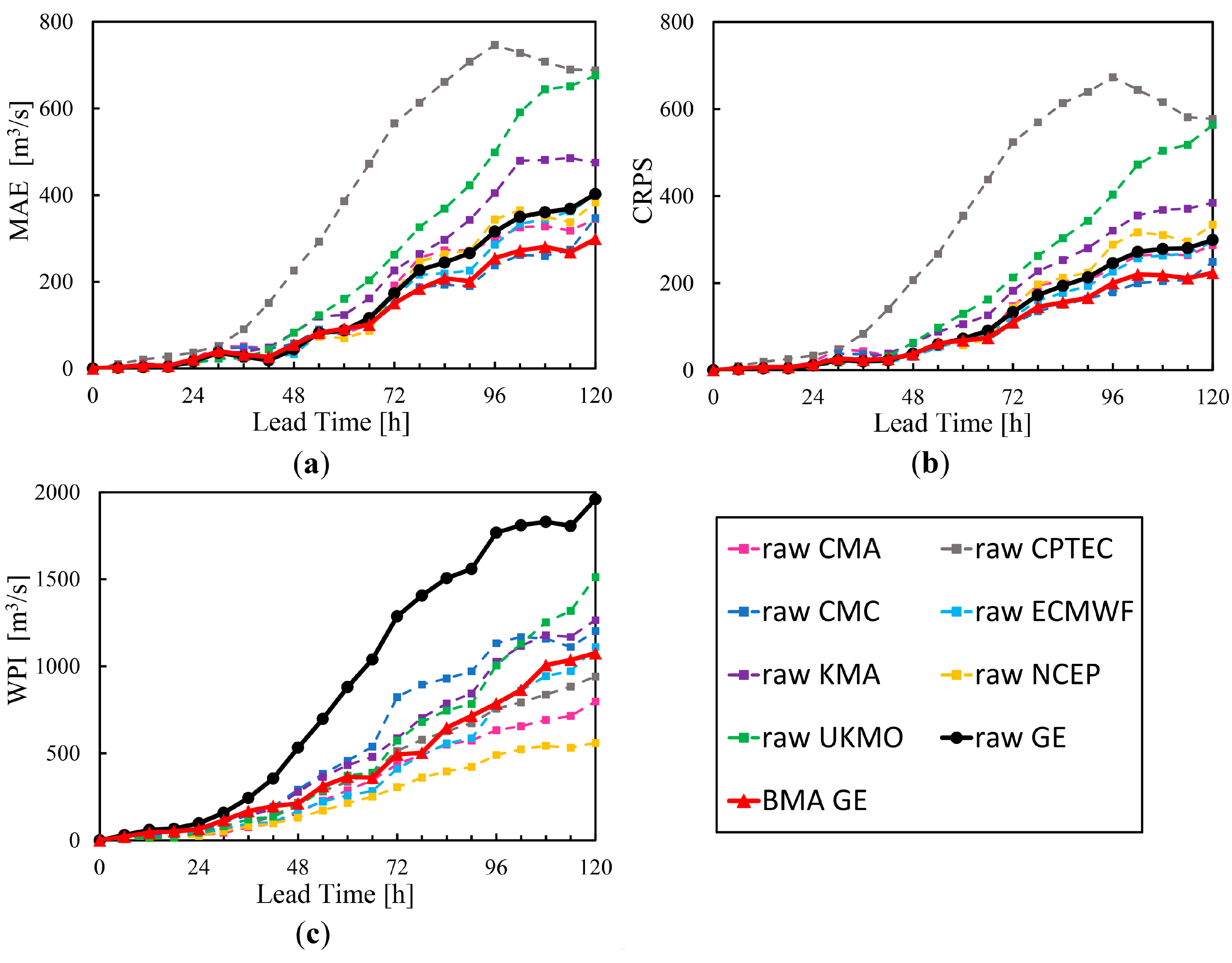
4.2.1. Analysis of Verification Metrics

Here, the three verification metrics mentioned above were employed, in order to assess calibration and sharpness. Figure 5 shows a simple comparison of BMA GE and raw GE runoff forecasts. Seven raw single-model ensemble (SE) runoff forecasts (derived from the same TIGGE EPSs) were also brought into the comparison. It is shown that all of the forecasts perform well at lead times below 24 h. Pappenberger et al. [40] point out that this is triggered by the watershed antecedent conditions, such as soil moisture and ground water levels, which have a much greater influence on the river discharge forecasts than meteorological conditions (mainly the precipitation), within short lead times (it seems to be 24 h for this study area). After a lead time of 24 h, differences among these forecasts start to emerge, and increase as lead times also increase. First, we investigated calibration, by the MAE and CRPS. Figure 5a,b indicates that BMA GE and raw CMC forecasts (both are approximately same) are much better calibrated, followed by raw ECMWF, raw CMA, and raw GE forecasts. The worst-performing forecast is the raw CPTEC forecast, which occupies the lowest position throughout the entire range of lead times. It is notable that the raw CMC forecast suddenly decreases at a lead time of 120 h, while BMA GE forecasts maintain their stabilization. Next, we focused on the sharpness. Figure 5c shows a different situation: the raw NCEP forecasts are the sharpest, and conversely to before, the raw GE forecasts perform the worst. BMA GE forecasts fall in between, belonging to a medium level, but are sharper than the raw CMC forecasts.

In summary, the investigations of calibration and sharpness presented above seem to suggest that for lead times of 6–24 h, all the forecasts have a similarly high accuracy; for lead times of 24–120 h, (1) raw GE forecasts have no advantage over raw SE forecasts, particularly when looking at sharpness; (2) BMA GE forecasts are more calibrated and sharper than raw GE forecasts; (3) BMA GE forecasts outperform any one of the raw SE forecasts, and are relatively stable and reliable.

4.2.2. Analysis of BMA Weights

BMA weights provide a measure of the relative usefulness of the individual ensemble members, and they can also be used as indicators of forecast performance, when ensemble members are sourced from different systems/models [12].

Table 2. Weights of seven contribution components for BMA GE probabilistic runoff forecasts. Owing to spatial confinements, this table shows only the weights at lead times of 24 h, 48 h, 72h, 96 h, 120 h.

Lead Time	Weights
	CMA	CPTEC	CMC	ECMWF	KMA	NCEP	UKMO
24 h	0.064	0.008	0.648	0.201	0.017	0.025	0.038
48 h	0.167	0.000	0.071	0.741	0.000	0.021	0.000
72 h	0.062	0.000	0.105	0.792	0.010	0.000	0.031
96 h	0.001	0.000	0.182	0.740	0.003	0.000	0.074
120 h	0.000	0.000	0.312	0.672	0.000	0.015	0.001

shows that raw CMC and raw ECMWF have the highest weights, and their ensemble members are the major contributiors of BMA GE predictive PDFs, which also means that both perform much better than the other raw SEs. These results are in accordance with the conclusions illustrated in the last subsection. One thing to note here is that there are inevitable errors in the BMA weights, because of the local convergence of the parameter estimation method, but fortunately, the errors are relatively minimal, and have little effect on the experimental results.

Taken from another perspective, these findings seem to partly explain why BMA GE forecasts have superiority over raw GE forecasts. As mentioned above, the simple arithmetic averaging method considers all of the ensemble members as equal, resulting in the prediction accuracy of raw GE being extremely vulnerable to weak members. Besides, such a combined approach easily gives rise to an excessively wide prediction interval, and thus affects the flood control decision-making. On the contrary, the BMA post-processing method is capable of distinguishing and eliminating the weak forecasts in the ensemble, by giving them very small weights, while providing an improvement for sharpness, due to the reduced ensemble size.

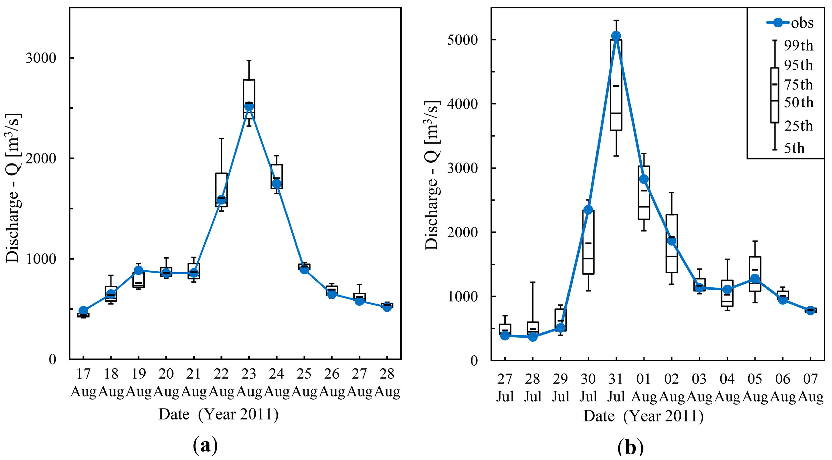
4.2.3. Analysis of Percentile Forecasts

The BMA post-processing method has the additional advantage, by generating a calibrated and sharp predictive PDF, of being able to provide a reliable description of the total predictive uncertainty [19,20]. Thus, theoretically, any possible flooding events can be captured through analyzing the PDF. In the following stage, we investigated the percentile forecasts of BMA GE at a lead time of 48 h, using two flooding events that took place in the verification period as examples. Interestingly, the two events have very different hydrological characteristics: Event I is a common flood with a peak of 2518 m³/s, while Event II has almost double the flood crest, which rises and drops steeply.

Figure 6a illustrates that the observed values are in close proximity to the 50th percentile forecasts (BMA GE deterministic river discharge forecasts). Yet, for event II, Figure 6b indicates that observations are far from the deterministic forecasts, and located near the 95th percentile forecasts, at both the rising limbs and peak, and the 80th percentile forecasts, at the falling limb. It is important to note that, in both flooding events, basically all of the observations fall within the 90% prediction interval of BMA GE, which seems to demonstrate that BMA GE probabilistic river discharge predictions are superior to the deterministic forecasts, and are able to provide a basis for taking precautions against common or severe flooding events in the Fu River basin. In addition, based on this analysis, we tentatively put forward an extreme flood warning scheme: consider the 90th percentile forecasts, instead of the 50th percentile forecasts, as the reference of flood warning, if the upper bound of the 90% prediction interval exceeds a specified threshold for some time (5000 m³/s in term of Event II).

5. Conclusions

In this paper, we applied the BMA post-processing method to the multi-model GE hydrologic prediction system, formed by coupling seven different TIGGE EPSs with the Xinanjiang hydrologic model, and dynamically set up a BMA GE probabilistic runoff forecasting experiment in the Fu River basin in China, during the period from 1 June to 31 August 2011. Some measures, such as data transformation and high-dimensional optimization, were taken in the experiment after considering the practical water regime and data conditions. The experimental results were examined and evaluated, using three measurements: verification metrics, BMA weights, and percentile forecasts, calculated for the entire verification period. It is shown that the BMA statistical post-processing method can bring about a significant improvement in calibration and sharpness for raw GE forecasts, and is also the best predictive skill in comparison with raw SE forecasts, over a range of lead times from 24 to 120 h. The reason for this result becomes clear in the discussion of BMA weights. The analysis of percentile forecasts during two different flooding events, demonstrates that BMA GE probabilistic runoff forecasts are more reliable and valuable than the deterministic forecasts, and have the capability to offer high-precision warning information for severe flooding events. Finally, an extreme flood warning scheme for the study area was proposed.

This study was based on the limited amount of hydrologic data collected within a year. Some research achievements, such as the extreme flood warning scheme, may not be suitable in practice until similarly regular patterns are found in additional studies [19]. Table 1 shows that the TIGGE ensemble forecasts provide an opportunity to allow lead times of up to 240 h, yet only the first 120 h were used in the study. So, it is necessary to carry out an extension of the current BMA GE runoff forecasting experiment, in order to explore the prediction quality at lead times ranging from 126 to 240 h. Additionally, it can be expected that the EM algorithm, limited by its inherent defect of local convergence, inevitably weakened the performance of BMA GE forecasts, even though the improvement measures have been applied. The other used-widely method, the MCMC algorithm, can effectively overcome this problem and converge to form global optimal solutions, but unfortunately, it usually suffers from poor computation efficiency [11]. Hence, an advanced parameter estimation method for the BMA model should be developed. Finally, Bogner et al. [41], and Hemri, Fundel, and Zappa [22], point out that the independence assumption of different lead times, usually leads to highly inconsistent forecasts, and thus affects the reliability of the forecasting system. In the future, a similar BMA study needs to account for the correlation structure between different lead times.

References

1. Roulin, E. Skill and relative economic value of medium-range hydrological ensemble predictions. Hydrol. Earth Syst. Sci. Discuss. 2006, 3, 1369–1406. [Google Scholar] [CrossRef]
2. Goswami, M.; O’connor, K.; Bhattarai, K. Development of regionalisation procedures using a multi-model approach for flow simulation in an ungauged catchment. J. Hydrol. 2007, 333, 517–531. [Google Scholar] [CrossRef]
3. Barnston, A.G.; Mason, S.J.; Goddard, L.; Dewitt, D.G.; Zebiak, S.E. Multimodel ensembling in seasonal climate forecasting at IRI. Bull. Am. Meteorol. Soc. 2003, 84, 1783–1796. [Google Scholar] [CrossRef]
4. Palmer, T.; Alessandri, A.; Andersen, U.; Cantelaube, P. Development of a European multimodel ensemble system for seasonal-to-interannual prediction (Demeter). Bull. Am. Meteorol. Soc. 2004, 85, 853–872. [Google Scholar] [CrossRef]
5. Doblas-Reyes, F.J.; Hagedorn, R.; Palmer, T. The rationale behind the success of multi-model ensembles in seasonal forecasting—II. Calibration and combination. Tellus A 2005, 57, 234–252. [Google Scholar] [CrossRef]
6. Hagedorn, R.; Doblas-Reyes, F.J.; Palmer, T. The rationale behind the success of multi-model ensembles in seasonal forecasting—I. Basic concept. Tellus A 2005, 57, 219–233. [Google Scholar] [CrossRef]
7. Cloke, H.L.; Pappenberger, F. Ensemble flood forecasting: A review. J. Hydrol. 2009, 375, 613–626. [Google Scholar] [CrossRef]
8. Pappenberger, F.; Bartholmes, J.; Thielen, J.; Cloke, H.L.; Buizza, R.; de Roo, A. New dimensions in early flood warning across the globe using grand-ensemble weather predictions. Geophys. Res. Lett. 2008, 35. [Google Scholar] [CrossRef]
9. He, Y.; Wetterhall, F.; Bao, H.; Cloke, H.; Li, Z.; Pappenberger, F.; Hu, Y.; Manful, D.; Huang, Y. Ensemble forecasting using TIGGE for the July–September 2008 floods in the upper huai catchment: A case study. Atmos. Sci. Lett. 2010, 11, 132–138. [Google Scholar] [CrossRef]
10. Xu, J.; Zhang, W.; Zheng, Z.; Jiao, M.; Chen, J. Early flood warning for Linyi watershed by the GRAPES/XXT model using TIGGE data. Acta Meteorol. Sin. 2012, 26, 103–111. [Google Scholar] [CrossRef]
11. Tian, X.; Xie, Z.; Wang, A.; Yang, X. A new approach for bayesian model averaging. Sci. China Earth Sci. 2012, 55, 1336–1344. [Google Scholar] [CrossRef]
12. Raftery, A.E.; Gneiting, T.; Balabdaoui, F.; Polakowski, M. Using bayesian model averaging to calibrate forecast ensembles. Mon. Weather Rev. 2005, 133, 1155–1174. [Google Scholar] [CrossRef]
13. Wilson, L.J.; Beauregard, S.; Raftery, A.E.; Verret, R. Calibrated surface temperature forecasts from the Canadian ensemble prediction system using bayesian model averaging. Mon. Weather Rev. 2007, 135, 1364–1385. [Google Scholar] [CrossRef]
14. Vrugt, J.A.; Clark, M.P.; Diks, C.G.; Duan, Q.; Robinson, B.A. Multi-objective calibration of forecast ensembles using bayesian model averaging. Geophys. Res. Lett. 2006, 33. [Google Scholar] [CrossRef]
15. Sloughter, J.M.L.; Raftery, A.E.; Gneiting, T.; Fraley, C. Probabilistic quantitative precipitation forecasting using bayesian model averaging. Mon. Weather Rev. 2007, 135, 3209–3220. [Google Scholar] [CrossRef]
16. Sloughter, J.M.; Gneiting, T.; Raftery, A.E. Probabilistic wind speed forecasting using ensembles and bayesian model averaging. J. Am. Stat. Assoc. 2010, 105, 25–35. [Google Scholar] [CrossRef]
17. Schmeits, M.J.; Kok, K.J. A comparison between raw ensemble output, (modified) bayesian model averaging, and extended logistic regression using ECMWF ensemble precipitation reforecasts. Mon. Weather Rev. 2010, 138, 4199–4211. [Google Scholar] [CrossRef]
18. Yang, C.; Yan, Z.; Shao, Y. Probabilistic precipitation forecasting based on ensemble output using generalized additive models and bayesian model averaging. Acta Meteorol. Sin. 2012, 26, 1–12. [Google Scholar] [CrossRef]
19. Liu, J.; Xie, Z. BMA probabilistic quantitative precipitation forecasting over the huaihe basin using TIGGE multimodel ensemble forecasts. Mon. Weather Rev. 2014, 142, 1542–1555. [Google Scholar] [CrossRef]
20. Duan, Q.; Ajami, N.K.; Gao, X.; Sorooshian, S. Multi-model ensemble hydrologic prediction using bayesian model averaging. Adv. Water Resour. 2007, 30, 1371–1386. [Google Scholar] [CrossRef]
21. Ajami, N.K.; Duan, Q.; Sorooshian, S. An integrated hydrologic bayesian multimodel combination framework: Confronting input, parameter, and model structural uncertainty in hydrologic prediction. Water Resour. Res. 2007, 43. [Google Scholar] [CrossRef]
22. Hemri, S.; Fundel, F.; Zappa, M. Simultaneous calibration of ensemble river flow predictions over an entire range of lead times. Water Resour. Res. 2013, 49, 6744–6755. [Google Scholar] [CrossRef]
23. Zhao, R. The Xinanjiang model applied in China. J. Hydrol. 1992, 135, 371–381. [Google Scholar]
24. Zhao, R.; Liu, X.; Singh, V. The Xinanjiang model. In Computer Models of Watershed Hydrology; Water Resources Publications: Fort Collins, CO, USA, 1995; pp. 215–232. [Google Scholar]
25. Bougeault, P.; Toth, Z.; Bishop, C.; Brown, B.; Burridge, D.; Chen, D.H.; Ebert, B.; Fuentes, M.; Hamill, T.M.; Mylne, K. The thorpex interactive grand global ensemble. Bull. Am. Meteorol. Soc. 2010, 91, 1059–1072. [Google Scholar] [CrossRef]
26. Swinbank, R.; Kyouda, M.; Buchanan, P.; Froude, L.; Hamill, T.M.; Hewson, T.D.; Keller, J.H.; Matsueda, M.; Methven, J.; Pappenberger, F. The TIGGE project and its achievements. Bull. Am. Meteorol. Soc. 2016, 97, 49–67. [Google Scholar] [CrossRef]
27. Duan, Q.; Sorooshian, S.; Gupta, V. Effective and efficient global optimization for conceptual rainfall-runoff models. Water Resour. Res. 1992, 28, 1015–1031. [Google Scholar] [CrossRef]
28. Dempster, A.P.; Laird, N.M.; Rubin, D.B. Maximum likelihood from incomplete data via the em algorithm. J. R. Stat. Soc. Ser. B 1977, 39, 1–38. [Google Scholar]
29. McLachlan, G.J.; Krishnan, T. The EM Algorithm and Extensions; Wiley: New York, NY, USA, 1997; p. 274. [Google Scholar]
30. Vrugt, J.A.; Diks, C.G.; Clark, M.P. Ensemble Bayesian model averaging using Markov chain Monte Carlo sampling. Environ. Fluid Mech. 2008, 8, 579–595. [Google Scholar] [CrossRef]
31. Vrugt, J.A.; Ter Braak, C.; Diks, C.; Robinson, B.A.; Hyman, J.M.; Higdon, D. Accelerating Markov chain Monte Carlo simulation by differential evolution with self-adaptive randomized subspace sampling. Int. J. Nonlinear Sci. Numer. Simul. 2009, 10, 273–290. [Google Scholar] [CrossRef]
32. Zsoter, E.; Pappenberger, F.; Smith, P.; Emerton, R.E.; Dutra, E.; Wetterhall, F.; Richardson, D.; Bogner, K.; Balsamo, G. Building a multi-model flood prediction system with the TIGGE archive. J. Hydrometeorol. 2016. [Google Scholar] [CrossRef]
33. Hemri, S.; Lisniak, D.; Klein, B. Multivariate postprocessing techniques for probabilistic hydrological forecasting. Water Resour. Res. 2015, 51, 7436–7451. [Google Scholar] [CrossRef]
34. Box, G.E.; Cox, D.R. An analysis of transformations. J. R. Stat. Soc. Ser. B (Methodol.) 1964, 26, 211–252. [Google Scholar]
35. Gneiting, T.; Balabdaoui, F.; Raftery, A.E. Probabilistic forecasts, calibration and sharpness. J. R. Stat. Soc. Ser. B 2007, 69, 243–268. [Google Scholar] [CrossRef]
36. Hersbach, H. Decomposition of the continuous ranked probability score for ensemble prediction systems. Weather Forecast. 2000, 15, 559–570. [Google Scholar] [CrossRef]
37. Gneiting, T.; Raftery, A.E. Strictly proper scoring rules, prediction, and estimation. J. Am. Stat. Assoc. 2007, 102, 359–378. [Google Scholar] [CrossRef]
38. Massey, F.J., Jr. The Kolmogorov-Smirnov test for goodness of fit. J. Am. Stat. Assoc. 1951, 46, 68–78. [Google Scholar] [CrossRef]
39. Fraley, C.; Raftery, A.E.; Gneiting, T. Calibrating multimodel forecast ensembles with exchangeable and missing members using bayesian model averaging. Mon. Weather Rev. 2010, 138, 190–202. [Google Scholar] [CrossRef]
40. Pappenberger, F.; Bartholmes, J.; Thielen, J.; Anghel, E. TIGGE: Medium Range Multi Model Weather Forecast Ensembles in Flood Forecasting (a Case Study); European Centre for Medium-Range Weather Forecasts: Reading, UK, 2008. [Google Scholar]
41. Bogner, K.; Pappenberger, F.; Cloke, H.L. Model combination and weighting methods in operational flood forecasting. In Proceedings of the EGU General Assembly Conference Abstracts, Vienna, Austria, 7–12 April 2013; Volume 15, p. 13629.
Figure 1. The location of the Yangtze River basin is shown in red and the Fu River basin in yellow (left); the general situations of the Fu River basin (right).
Water 09 00074 g001
Figure 2. The flow chart of the BMA GE probabilistic runoff forecasting system in the Fu River basin, showing a cascade of components. Note that this is not a standardized technological procedure, and some components may need to be modified/removed for other experiments.
Water 09 00074 g002
Figure 3. Normal probability plots of the original and Box-Cox transformed runoff data at a lead time of 48 h: (a) original data; (b) Box-Cox transformed data.
Water 09 00074 g003
Figure 4. Comparison of training period lengths for lead times ranging from 6 to 120 h: (a) mean MAE over the verification period; (b) mean CRPS over the verification period.
Water 09 00074 g004
Figure 5. Comparison of calibration and sharpness between BMA GE, raw GE, and raw SE forecasts: (a) mean MAE over the verification period; (b) mean CRPS over the verification period; (c) mean WPI over the verification period.
Water 09 00074 g005
Figure 6. BMA GE percentile forecasts and observed river discharge for two flooding events in the Fu River basin: (a) Event I; (b) Event II.
Water 09 00074 g006