
Assessment of Optional Sediment Transport Functions via the Complex Watershed Simulation Model SWAT

 , , , and
Abstract
:1. Introduction
2. Materials and Methods
2.1. The SWAT Model
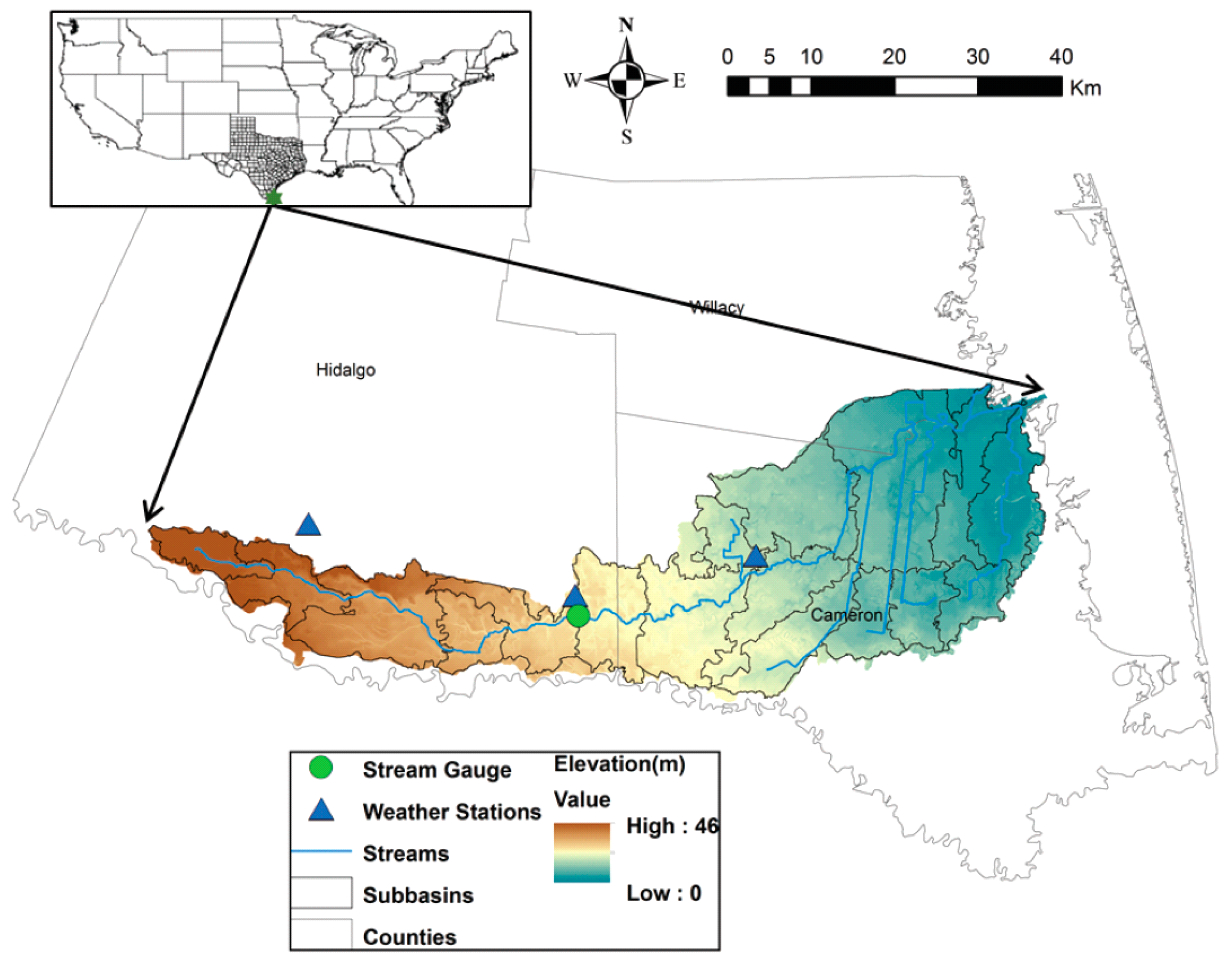
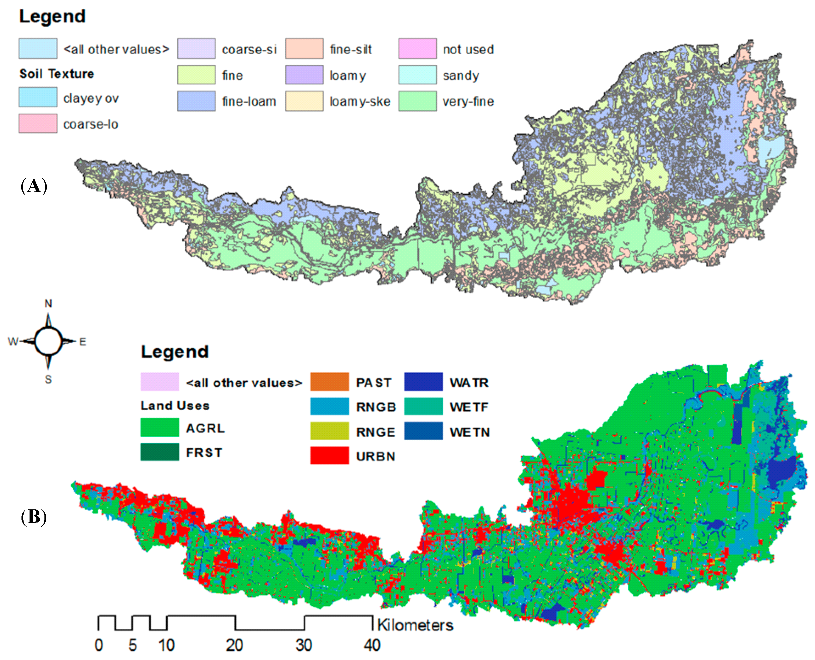
2.2. Study Area
2.3. Sources of Input Data
2.4. Sediment Transport Methods in SWAT
2.4.1. Modified Bagnold Equation
2.4.2. Kodoatie Equation
2.4.3. Molinas and Wu Equation
2.4.4. Yang Sand and Gravel Equation
2.5. Model Calibration and Validation
3. Results
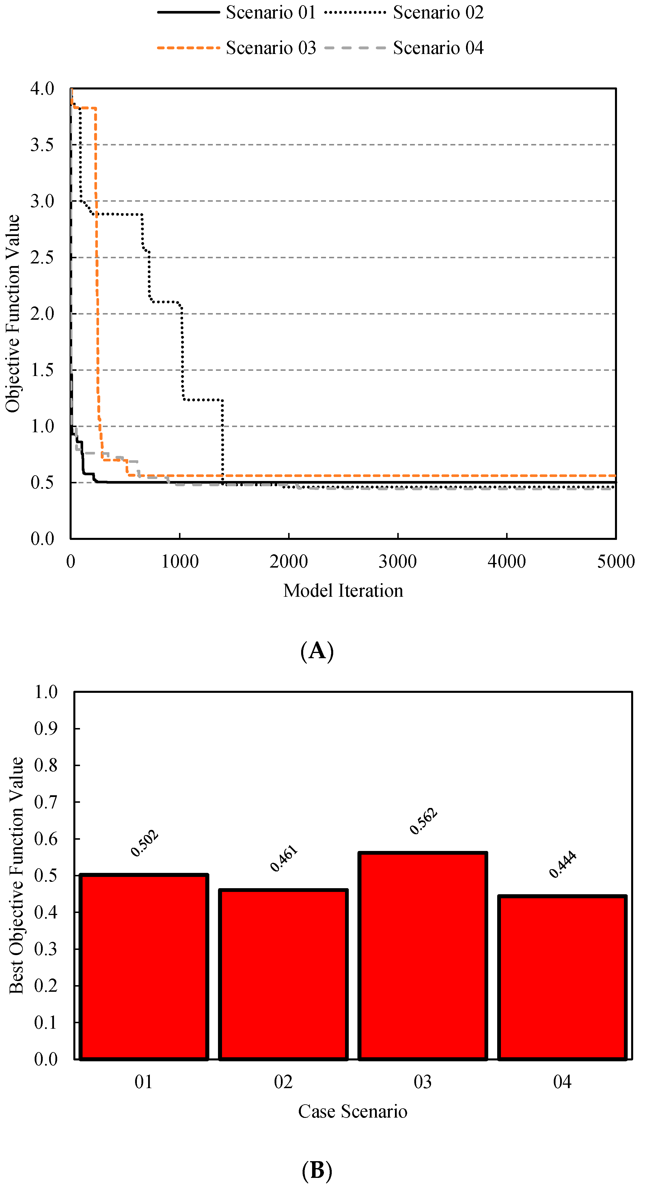
3.1. Comprehensive Comparisons by Objective Function Values
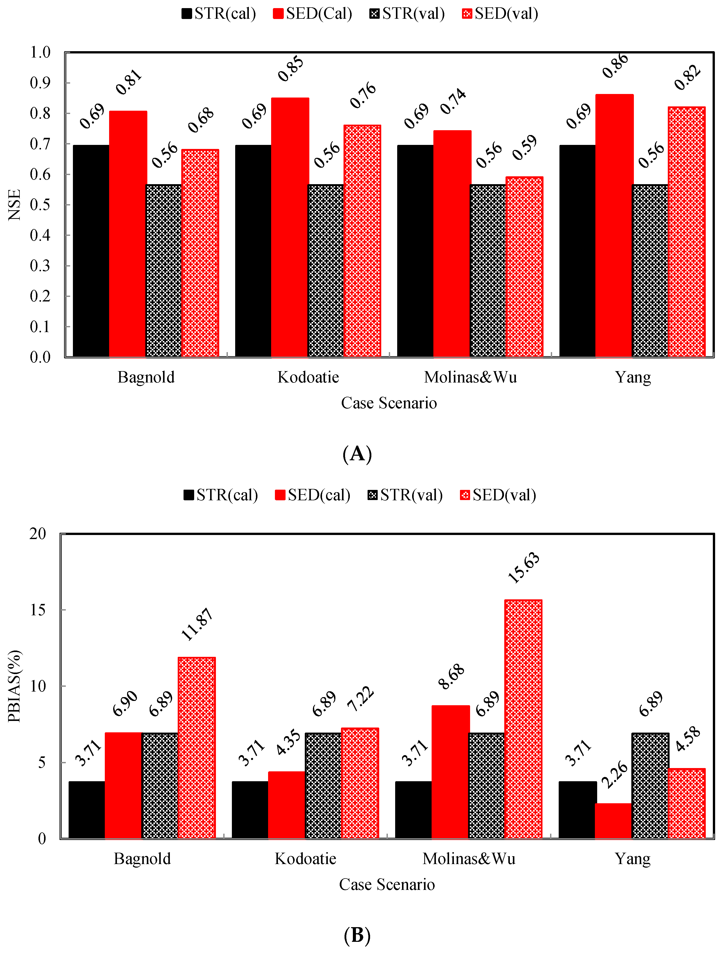
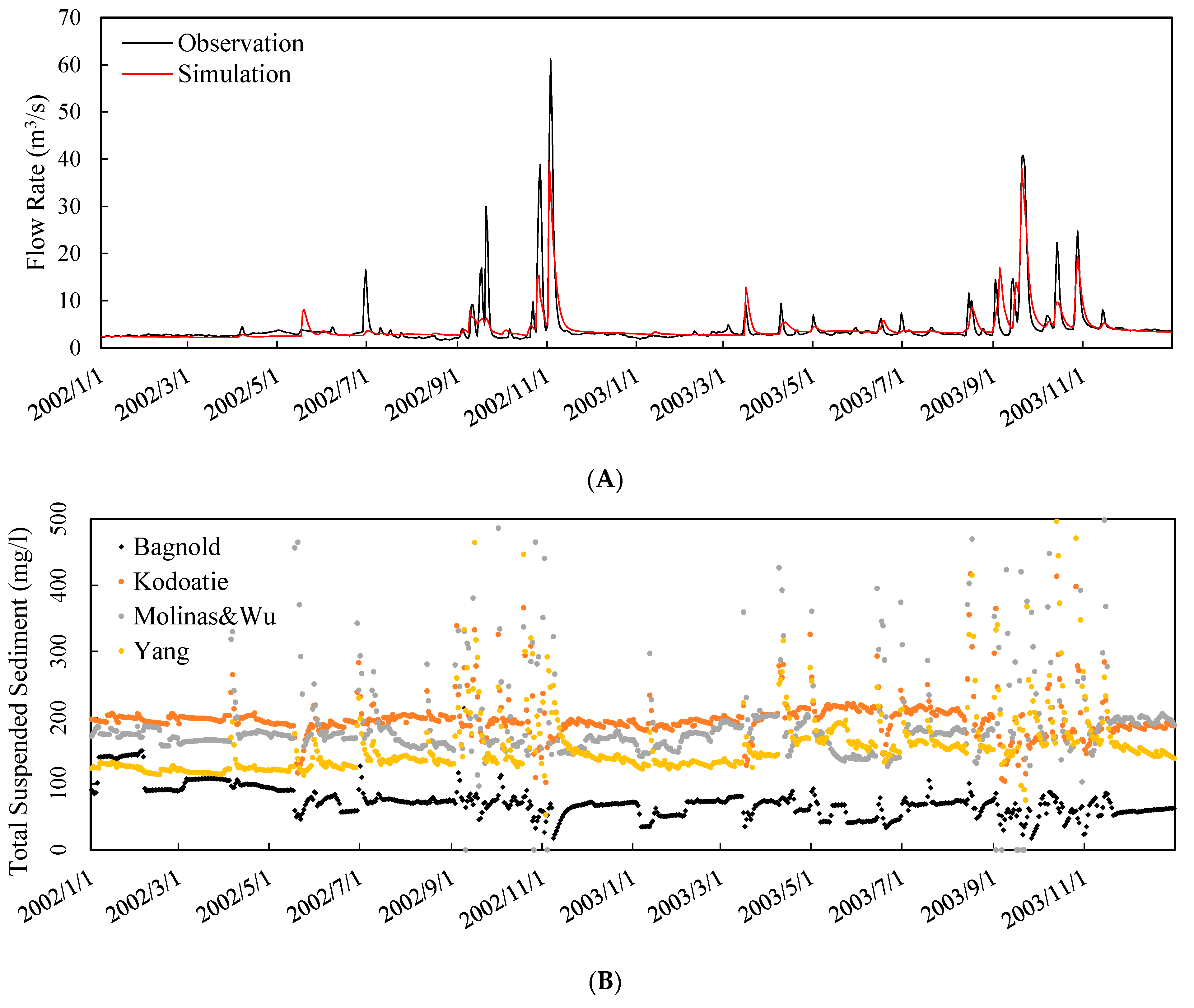
3.2. Evaluation of Model Performance on Streamflow and Sediment Predictions
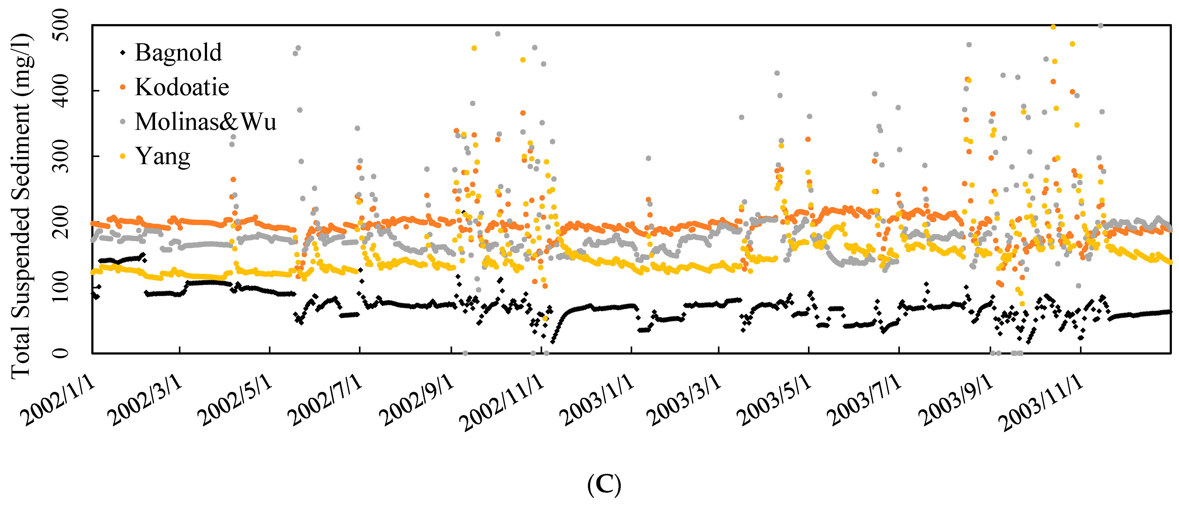
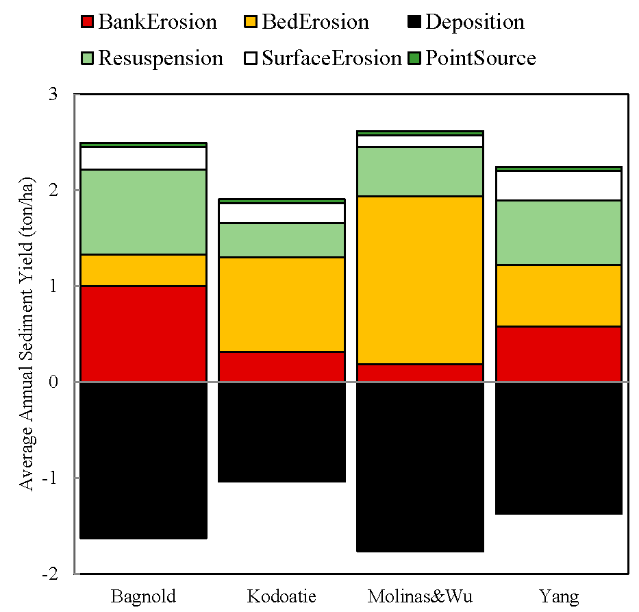
3.3. Evaluation of Sediment Concentration and Sediment Budget
3.4. Uncertainty Analysis
4. Discussion
4.1. Similarities and Differences during Calibration
4.2. Comparisons of Equation Theories and Applications
5. Conclusions
Acknowledgments
Author Contributions
Conflicts of Interest
Appendix A

| Parameters | Input File | Units | Range | Calibrated Values | Description |
|---|---|---|---|---|---|
| EPCO | .bsn | - | 0–1 | 0.454 | Plant uptake compensation factor |
| SURLAG | .bsn | Day | 1–24 | 6.865 | Surface runoff lag time |
| ALPHA_BF | .gw | 1/Day | 0–1 | 0.764 | Baseflow alpha factor |
| GW_DELAY | .gw | Day | 0–500 | 98.22 | Groundwater delay |
| GW_REVAP | .gw | - | 0.02–0.2 | 0.042 | Groundwater “revap” coefficient |
| GWQMN | .gw | mm H2O | 0–5000 | 28.16 | Threshold depth of water in the shallow aquifer required for return flow to occur |
| ESCO | .hru | - | 0–1 | 0.403 | Soil evaporation compensation factor |
| CN_F | .mgt | % | ±10 | 9.144 | Initial SCS CN II value |
| CH_K2 | .rte | mm/h | −0.01–500 | 85.60 | Effective hydraulic conductivity in main channel alluvium |
| CH_N2 | .rte | - | −0.01–0.3 | 0.070 | Manning’s “n” value for the main channel |
| SOL_AWC | .sol | % | ±10 | 8.522 | Available water capacity of the soil layer |
| SOL_K | .sol | % | ±10 | 8.997 | Saturated hydraulic conductivity |
| CH_K1 | .sub | mm/h | 0–300 | 32.06 | Effective hydraulic conductivity in tributary channel alluvium |
| CH_N1 | .sub | - | 0.01–30 | 0.191 | Manning’s “n” value for the tributary channels |
Appendix B
| Parameter | Input File | Unit | Scenario 01 | Scenario 02 | Scenario 03 | Scenario 04 | Range | Description |
|---|---|---|---|---|---|---|---|---|
| ADJ_PKR | .bsn | - | 0.549 | 0.464 | 1.290 | 1.195 | 0–2 | Peak rate adjustment factor for sediment routing in the sub-basin (tributary channels) |
| PRF | .bsn | - | 1.713 | 0.755 | 0.089 | 1.257 | 0–2 | Peak rate adjustment factor for sediment routing in the main channel |
| SPCON | .bsn | - | 0.0074 | 0.0067 | 0.0059 | 0.0067 | 0.0001–0.01 | Linear parameter for calculating the maximum amount of sediment that can be re-entrained during channel sediment routing |
| SPEXP | .bsn | - | 1.995 | 1.051 | 1.760 | 1.761 | 1.0–1.5 | Exponent parameter for calculating sediment re-entrained in channel sediment routing |
| CH_BED_BD | .rte | g/cc | 1.811 | 1.386 | 1.617 | 1.110 | 1.1–1.9 | Bulk density of channel bed sediment |
| CH_BED_D50 | .rte | μm | 4650 | 1.267 | 49.24 | 8241 | 1–10,000 | D50 median particle size diameter of channel bed sediment |
| CH_BNK_BD | .rte | g/cc | 1.118 | 1.118 | 1.335 | 1.172 | 1.1–1.9 | Bulk density of channel bank sediment |
| CH_BNK_D50 | .rte | μm | 2592 | 1868 | 1677 | 1550 | 1–10,000 | D50 median particle size diameter of channel bank sediment |
| CH_COV1 | .rte | - | 0.1807 | 3.7340 | 4.2880 | 4.4340 | 0–5 | Channel erodibility factor |
| CH_COV2 | .rte | - | 2.3600 | 0.0006 | 0.0528 | 0.4123 | 0–5 | Channel cover factor |
References
- Arnold, J.G.; Allen, P.M.; Bernhardt, G.A. Comprehensive surface-groundwater flow model. J. Hydrol. 1993, 142, 47–69. [Google Scholar] [CrossRef]
- Arnold, J.G.; Kiniry, J.R.; Srinivasan, R.; Williams, J.R.; Haney, E.B.; Neitsch, S.L. Soil and Water Assessment Tool Input/Output Documentation 2012; Texas Water Resources Institute Technical Report No. 439; Texas A&M University System: College Station, TX, USA, 2012. [Google Scholar]
- Niraula, R.; Kalin, L.; Wang, R.; Srivastava, P. Determining nutrient and sediment critical source areas with SWAT model: Effect of lumped calibration. Trans. ASABE 2012, 55, 137–147. [Google Scholar] [CrossRef]
- Johnson, M.V.V.; Norfleet, M.L.; Atwood, J.D.; Behrman, K.D.; Kiniry, J.R.; Arnold, J.G.; White, M.J.; Williams, J. The Conservation Effects Assessment Project (CEAP): A national scale natural resources and conservation needs assessment and decision support tool. IOP Conf. Ser. Earth Environ. Sci. 2015, 25. [Google Scholar] [CrossRef]
- Scavia, D.; Kalcic, M.; Muenich, R.L.; Aloysius, N.; Arnold, J.; Boles, C.; Confessor, R.; De Pinto, J.; Gildow, M.; Martin, J.; et al. Informing Lake Erie Agriculture Nutrient Management via Scenario Evaluation; University of Michigan: Ann Arbor, MI, USA, 2016; Available online: http://graham.umich.edu/water/project/erie-western-basin (accessed on 23 January 2017).
- Sharifi, A.; Kalin, L.; Hantush, M.M.; Isik, S.; Jordan, T. Carbon export and dynamics from flooded wetlands: A modeling approach. Ecol. Model. 2013, 263, 196–210. [Google Scholar] [CrossRef]
- Tasdighi, A.; Arabi, M.; Osmond, D.L. The relationship between land use and vulnerability to nitrogen and phosphorus pollution in an urban watershed. J. Environ. Qual. 2017, 46, 113–122. [Google Scholar] [CrossRef]
- Yen, H.; White, M.J.; Arnold, J.G.; Keitzer, S.C.; Johnson, M.V.; Atwood, J.D.; Daggupati, P.; Herbert, M.E.; Sowa, S.P.; Ludsin, S.A.; et al. Western Lake Erie Basin: Soft-data-constrained, NHDPlus resolution watershed modeling and exploration of applicable conservation scenarios. Sci. Total Environ. 2016, 569–570, 1265–1281. [Google Scholar] [CrossRef] [PubMed]
- Sharifi, A.; Lang, M.W.; McCarty, G.W.; Sadeghi, A.M.; Lee, S.; Yen, H.; Rabenhorst, M.C.; Jeong, J.; Yeo, I.-Y. Improving model prediction reliability through enhanced representation of wetland soil processes and constrained model auto calibration–A paired watershed study. J. Hydrol. 2016, 541, 1088–1103. [Google Scholar] [CrossRef]
- Gassman, P.W.; Sadeghi, A.M.; Srinivasan, R. Applications of the SWAT Model special section: Overview and insights. J. Environ. Qual. 2014, 43, 1–8. [Google Scholar] [CrossRef] [PubMed]
- Woodbury, J.D.; Shoemaker, C.A.; Easton, Z.M.; Cowan, D.M. Application of SWAT with and without Variable Source Area Hydrology to a Large Watershed. JAWRA J. Am. Water Resour. Assoc. 2014, 50, 42–56. [Google Scholar] [CrossRef]
- Carvalho-Santos, C.; Nunes, J.P.; Monteiro, A.T.; Hein, L.; Honrado, J.P. Assessing the effects of land cover and future climate conditions on the provision of hydrological services in a medium-sized watershed of Portugal. Hydrol. Process. 2016, 30, 720–738. [Google Scholar] [CrossRef]
- Bärlund, I.; Kirkkala, T.; Malve, O.; Kämäri, J. Assessing SWAT model performance in the evaluation of management actions for the implementation of the Water Framework Directive in a Finnish catchment. Environ. Model. Softw. 2007, 22, 719–724. [Google Scholar] [CrossRef]
- Flynn, K.F.; Van Liew, M.W. Evaluation of swat for sediment prediction in a mountainous snowmelt-dominated catchment. Trans. ASABE 2011, 54, 113–122. [Google Scholar] [CrossRef]
- Mishra, A.; Kar, S. Modeling hydrologic processes and NPS pollution in a small watershed in subhumid subtropics using SWAT. J. Hydrol. Eng. 2012, 17, 445–454. [Google Scholar] [CrossRef]
- Lam, Q.; Schmalz, B.; Fohrer, N. The impact of agricultural Best Management Practices on water quality in a North German lowland catchment. Environ. Monit. Assess. 2011, 183, 351–379. [Google Scholar] [CrossRef] [PubMed]
- Wu, Y.; Chen, J. Modeling of soil erosion and sediment transport in the East River Basin in Southern China. Sci. Total Environ. 2012, 441, 159–168. [Google Scholar] [CrossRef] [PubMed]
- Walling, D.E. The sediment delivery problem. J. Hydrol. 1983, 65, 209–237. [Google Scholar] [CrossRef]
- Lu, S.; Kayastha, N.; Thodsen, H.; van Griensven, A.; Andersen, H.E. Multiobjective Calibration for Comparing Channel Sediment Routing Models in the Soil and Water Assessment Tool. J. Environ. Qual. 2014, 43, 110–120. [Google Scholar] [CrossRef] [PubMed]
- Walling, D.E. The Impact of Global Change on Erosion and Sediment Transport by Rivers: Curretn Progress and Future Challenges; World Water Assessment Programme; United Nation Educational, Scientific and Cultural Organization: Paris, France, 2009. [Google Scholar]
- Bagnold, R.A. Bed load transport by natural rivers. Water Resour. Res. 1977, 13, 303–312. [Google Scholar] [CrossRef]
- Neitsch, S.L.; Arnold, J.G.; Kiniry, J.R.; Williams, J.R. Soil and Water Assessment Tool Theoretical Documentation Version 2009; Texas Water Resources Institute Technical Report No. 406; Texas A&M University System: College Station, TX, USA, 2011. [Google Scholar]
- Kodoatie, R.J. Sediment Transport Relations in Alluvial Channels. Ph.D. Thesis, Colorado State University, Fort Collins, CO, USA, 2000. [Google Scholar]
- Molinas, A.; Wu, B.S. Transport of sediment in large sand-bed rivers. J. Hydraul. Res. 2001, 39, 135–146. [Google Scholar] [CrossRef]
- Yang, C.T. Sediment Transport Theory and Practice; The McGraw-Hill Companies, Inc.: New York, NY, USA, 1996. [Google Scholar]
- Williams, J.R. SPNM, a model for predicting sediment, phosphorus, and nitrogn yields from agricultural basins. Water Resour. Bull. 1980, 16, 843–848. [Google Scholar] [CrossRef]
- Lu, S.; Kronvang, B.; Audet, J.; Trolle, D.; Andersen, H.E.; Thodsen, H.; van Griensven, A. Modelling sediment and total phosphorus export from a lowland catchment: Comparing sediment routing methods. Hydrol. Process. 2014. [Google Scholar] [CrossRef]
- Wang, R.; Bowling, L.C.; Cherkauer, K.A. Estimation of the effects of climate variability on crop yield in the Midwest USA. Agric. For. Meteorol. 2016, 216, 141–156. [Google Scholar] [CrossRef]
- Jha, M.K.; Gassman, P.W.; Arnold, J.G. Water quality modeling for the Raccoon River watershed using SWAT. Trans. ASAE 2007, 50, 479–493. [Google Scholar] [CrossRef]
- Hoque, Y.M.; Hantush, M.M.; Govindaraju, R.S. On the scaling behavior of reliability-resilience-vulnerability indices in agricultural watersheds. Ecol. Indic. 2014, 40, 136–146. [Google Scholar] [CrossRef]
- Wang, R.; Kalin, L. Responses of hydrological processes and water quality to land use/cover (LULC) and climate change in a coastal watershed. In Proceedings of the Second International Conference on Sustainable Systems and the Environment (ISSE’14), Sharjah, United Arab Emirates, 12–13 February 2014.
- Butcher, J.B.; Johnson, T.E.; Nover, D.; Sarkar, S. Incorporating the effects of increased atmospheric CO2 in watershed model projections of climate change impacts. J. Hydrol. 2014, 513, 322–334. [Google Scholar] [CrossRef]
- Daggupati, P.; Yen, H.; White, M.J.; Srinivasan, R.; Arnold, J.G.; Keitzer, C.S.; Sowa, S.P. Impact of model development, calibration and validation decisions on hydrological simulations in West Lake Erie Basin. Hydrol. Process. 2015. [Google Scholar] [CrossRef]
- Wang, R.; Bowling, L.C.; Cherkauer, K.A.; Raj, C.; Her, Y.; Chaubey, I. Biophysical and hydrological effects of future climate change including trends in CO2, in the St. Joseph River watershed, Eastern Corn Belt. Agric. Water Manag. 2016. [Google Scholar] [CrossRef]
- White, M.; Harmel, D.; Yen, H.; Arnold, J.; Gambone, M.; Haney, R. Development of Sediment and Nutrient Export Coefficients for U.S. Ecoregions. JAWRA J. Am. Water Resour. Assoc. 2015, 1–18. [Google Scholar] [CrossRef]
- Wang, R.; Kalin, L.; Kuang, W.; Tian, H. Individual and combined effects of land use/cover and climate change on Wolf Bay Watershed Streamflow in Southern Alabama. Hydrol. Process. 2014. [Google Scholar] [CrossRef]
- Kannan, N. SWAT Modeling of the Arroyo Colorado Watershed; TR-426; Texas Water Resources Institute: College Station, TX, USA, 2012. [Google Scholar]
- Seo, M.-J.; Yen, H.; Jeong, J. Transferability of input parameters between SWAT 2009 and SWAT 2012. J. Environ. Qual. 2014, 43, 869–880. [Google Scholar] [CrossRef] [PubMed]
- National Elevation Dataset. U.S. Geological Survey (USGS). Available online: http://ned.usgs.gov/ (accessed on 12 October 2016).
- Gesch, D.; Evans, G.; Mauck, J.; Hutchinson, J.; Carswell, W.J., Jr. The National Map—Elevation: U.S. Geological Survey Fact Sheet 2009-3053. 2009; 4p. Available online: http://ned.usgs.gov/ (accessed on 18 September 2013). [Google Scholar]
- Rains, T.H.; Miranda, R.M. Simulation of Flow and Water Quality of the Arroyo Colorado, Texas, 1989–1999; United States Geological Survey-Water Resources Investigations Report, No: 02-4110; United States Geological Survey: Reston, VA, USA, 2002.
- Harmel, R.D.; Cooper, R.J.; Slade, R.M.; Haney, R.L.; Arnold, J.G. Cumulative uncertainty in measured streamflow and water quality data for small watersheds. Trans. ASABE 2006, 49, 689–701. [Google Scholar] [CrossRef]
- Yen, H.; Hoque, Y.; Wang, X.; Harmel, R.D. Applications of Explicitly-Incorporated/Post-Processing Measurement Uncertainty in Watershed Modeling. JAWRA J. Am. Water Resour. Assoc. 2016, 52, 523–540. [Google Scholar] [CrossRef]
- Runkel, R.; Crawford, C.; Cohn, T. Load ESTimator (LOADEST): A FORTRAN program for estimating constituent loads in streams and rivers. In US Geological Survey Techniques and Methods Book 4; US Geological Survey: Reston, VA, USA, 2004. [Google Scholar]
- Eaton, B.C.; Millar, R.G. Optimal alluvial channel width under a bank stability constraint. Geomorphology 2004, 62, 35–45. [Google Scholar] [CrossRef]
- Posada, G.L. Transport of Sands in Deep Rivers. Ph.D. Thesis, Department of Civil Engineering, Colorado State University, Fort Collins, CO, USA, 1995. [Google Scholar]
- Yang, C.T. Incipient motion and sediment transport. J. Hydraul. Div. 1973, 99, 1679–1704. [Google Scholar]
- Yang, C.T. Unit stream power equation for gravel. J. Hydraul. Div. 1984, 110, 1783–1797. [Google Scholar] [CrossRef]
- Yen, H.; Wang, X.; Fontane, D.G.; Harmel, R.D.; Arabi, M. A framework for propagation of uncertainty contributed by parameterization, input data, model structure, and calibration/validation data in watershed modeling. Environ. Model. Softw. 2014, 54, 211–221. [Google Scholar] [CrossRef]
- Yen, H. Confronting Input, Parameter, Structural, and Measurement Uncertainty in Multi-Site Multiple Responses Watershed Modeling Using Bayesian Inferences. Ph.D. Thesis, Colorado State University, Fort Collins, CO, USA, 2012. [Google Scholar]
- Yen, H.; Jeong, J.; Tseng, W.; Kim, M.; Records, R.; Arabi, M. Computational procedure for evaluating sampling techniques on watershed model calibration. J. Hydrol. Eng. 2014. [Google Scholar] [CrossRef]
- American Society of Civil Engineers (ASCE). Criteria for evaluation of watershed models, ASCE task committee on definition of criteria for evaluation of watershed models of the watershed management, irrigation, and drainage division. J. Irrig. Drain. Eng. 1993, 119, 429. [Google Scholar]
- Servat, E.; Dezetter, A. Selection of calibration objective functions in the context of rainfall-runoff modeling in a Sudanese savannah area. Hydrol. Sci. J. 1991, 36, 307–330. [Google Scholar] [CrossRef]
- Moriasi, D.N.; Arnold, J.G.; Liew, M.W.V.; Bingner, R.L.; Harmel, R.D.; Veith, T.L. Model evaluation guidelines for systematic quantification of accuracy in watershed simulations. Trans. ASABE 2007, 50, 885–900. [Google Scholar] [CrossRef]
- Moriasi, D.N.; Gitau, M.W.; Pai, N.; Daggupati, P. Hydrologic and water quality models: Performance measures and evaluation criteria. Trans. ASABE 2015, 58, 1763–1785. [Google Scholar]
- Yen, H.; White, M.J.; Jeong, J.; Arabi, M.; Arnold, J.G. Evaluation of alternative surface runoff accounting procedures using the SWAT model. Int. J. Agric. Biol. Eng. 2015, 8, 54–68. [Google Scholar]
- Fox, J.F.; Davis, C.M.; Martin, D.K. Sediment source assessment in a lowland watershed using nitrogen stable isotopes. JAWRA J. Am. Water Res. Assoc. 2010, 46, 1192–1204. [Google Scholar] [CrossRef]
- Mukundan, R.; Radcliffe, D.E.; Ritchie, J.C.; Risse, L.M.; McKinley, R.A. Sediment fingerprinting to determine the source of suspended sediment in a southern Piedmont stream. J. Environ. Qual. 2010, 39, 1328–1337. [Google Scholar] [CrossRef] [PubMed]
- Wu, B.; Van Maren, D.; Li, L. Predictability of sediment transport in the Yellow River using selected transport formulas. Int. J. Sediment Res. 2008, 23, 283–298. [Google Scholar] [CrossRef]
- United States Department of Agriculture-National Resources Conservation Service (USDA-NRCS). United States Department of Agriculture-National Resources Conservation Service (USDA-NRCS). Chapter 10: Estimation of direct runoff from storm rainfall. In Part 630: Hydrology: NRCS National Engineering Handbook; USDA National Resources Conservation Service: Washington, DC, USA, 2004. [Google Scholar]
- Green, W.H.; Ampt, G.A. Studies on soil physics, part I, the flow of air and water through soils. J. Agric. Sci. 1911, 4, 1–24. [Google Scholar]


| Scenario | Inclusion Rate (%) | Spread | ||
|---|---|---|---|---|
| Streamflow | Sediment | Streamflow | Sediment | |
| Scenario 01 | 49.59 | 62.50 | 1.815 | 0.046 |
| Scenario 02 | 49.59 | 35.42 | 1.815 | 0.033 |
| Scenario 03 | 49.59 | 54.17 | 1.815 | 0.040 |
| Scenario 04 | 49.59 | 31.25 | 1.815 | 0.029 |
© 2017 by the authors. Licensee MDPI, Basel, Switzerland. This article is an open access article distributed under the terms and conditions of the Creative Commons Attribution (CC BY) license ( http://creativecommons.org/licenses/by/4.0/).
Share and Cite
Yen, H.; Lu, S.; Feng, Q.; Wang, R.; Gao, J.; Brady, D.M.; Sharifi, A.; Ahn, J.; Chen, S.-T.; Jeong, J.; et al. Assessment of Optional Sediment Transport Functions via the Complex Watershed Simulation Model SWAT. Water 2017, 9, 76. https://doi.org/10.3390/w9020076
Yen H, Lu S, Feng Q, Wang R, Gao J, Brady DM, Sharifi A, Ahn J, Chen S-T, Jeong J, et al. Assessment of Optional Sediment Transport Functions via the Complex Watershed Simulation Model SWAT. Water. 2017; 9(2):76. https://doi.org/10.3390/w9020076
Chicago/Turabian StyleYen, Haw, Shenglan Lu, Qingyu Feng, Ruoyu Wang, Jungang Gao, Dawn Michelle Brady, Amirreza Sharifi, Jungkyu Ahn, Shien-Tsung Chen, Jaehak Jeong, and et al. 2017. "Assessment of Optional Sediment Transport Functions via the Complex Watershed Simulation Model SWAT" Water 9, no. 2: 76. https://doi.org/10.3390/w9020076